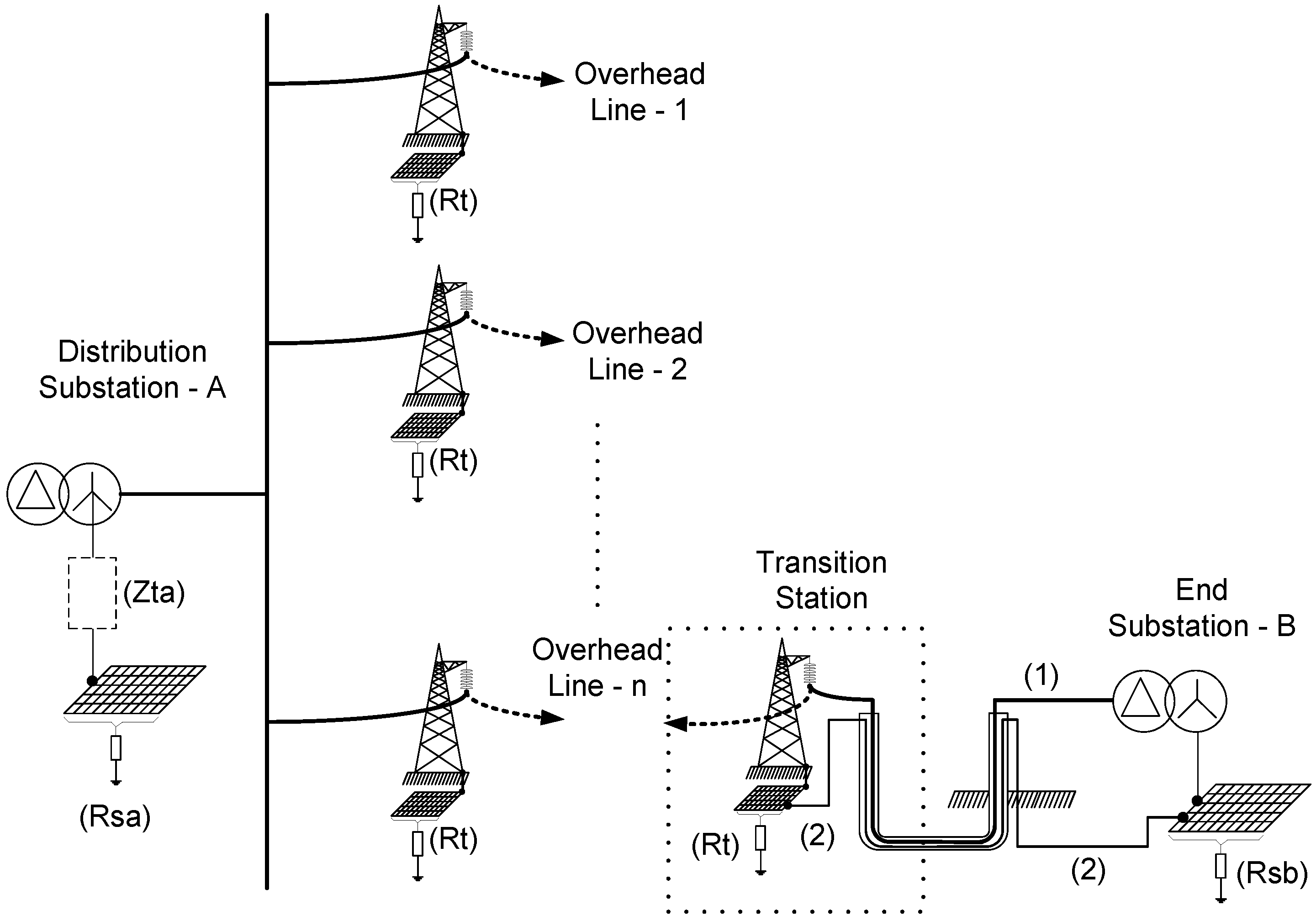
Figure 1.
Power distribution network with transition cable-overhead line. (1) Active conductor of power cables; (2) Shields of the power cable; (Rt) Tower ground resistance; (Rsa) Ground resistance of distribution substation-A; (Rsb) Ground resistance of end substation-B; (Zta) Grounding impedance.
Figure 1.
Power distribution network with transition cable-overhead line. (1) Active conductor of power cables; (2) Shields of the power cable; (Rt) Tower ground resistance; (Rsa) Ground resistance of distribution substation-A; (Rsb) Ground resistance of end substation-B; (Zta) Grounding impedance.
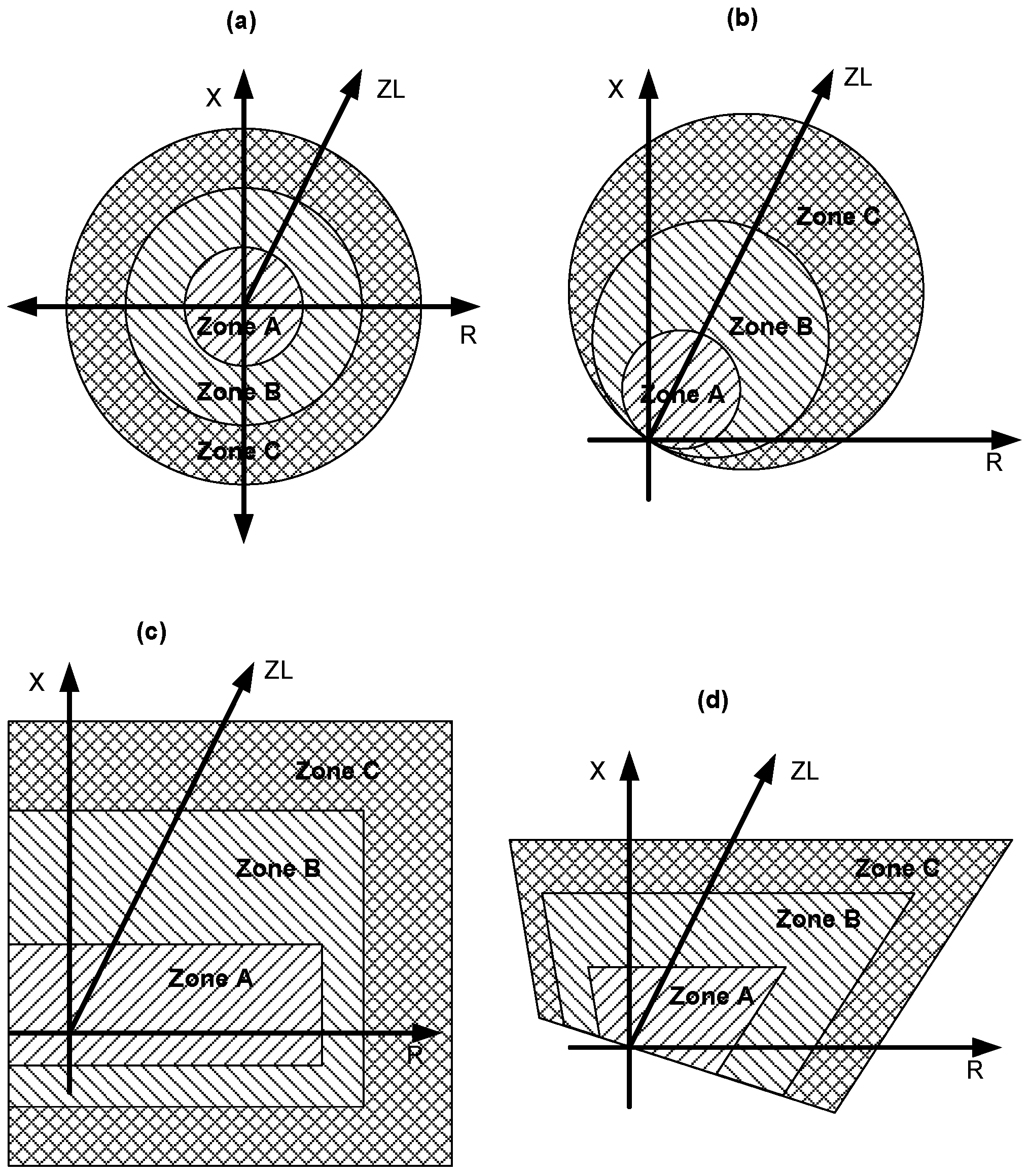
Figure 2.
Types of impedance relay characteristics with three zone settings: (a) Impedance relay; (b) Mho relay; (c) Reactance relay; (d) Quadrilateral relay.
Figure 2.
Types of impedance relay characteristics with three zone settings: (a) Impedance relay; (b) Mho relay; (c) Reactance relay; (d) Quadrilateral relay.
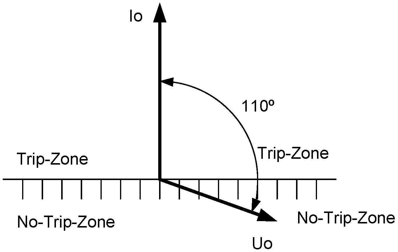
Figure 3.
Tripping zone for solidly grounded power distribution networks. (Uo) Residual voltage; (Io) Residual current; (110°) Characteristic tripping angle.
Figure 3.
Tripping zone for solidly grounded power distribution networks. (Uo) Residual voltage; (Io) Residual current; (110°) Characteristic tripping angle.
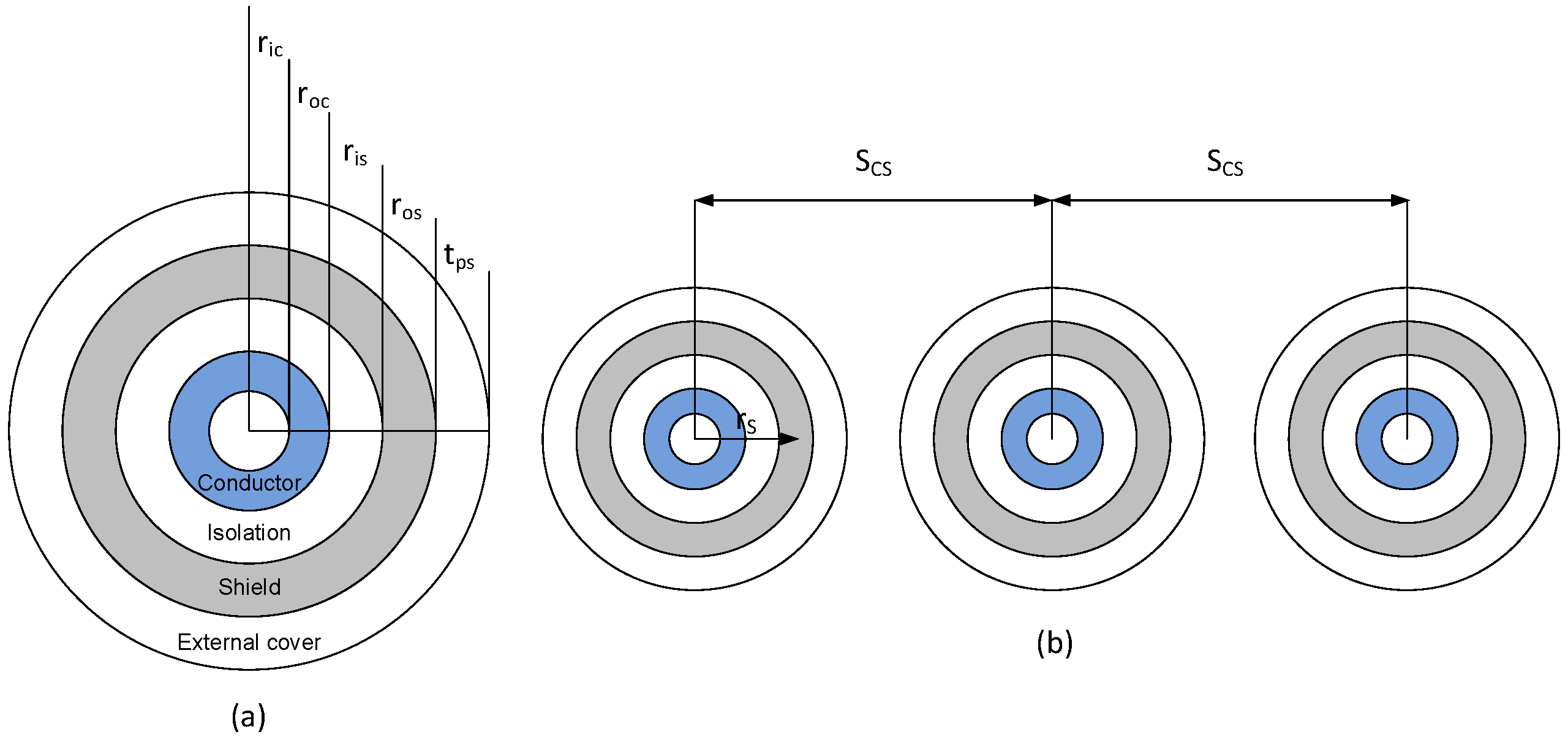
Figure 4.
(a) Cable composition and (b) flat disposal. (ric) Internal conductor radius; (roc) External conductor radius; (ris) Internal conductor shield; (ros) External shield radius; (rs) Average shield radius; (SCS) Distance between axes of the conductor and shield; (tps) External cover thickness.
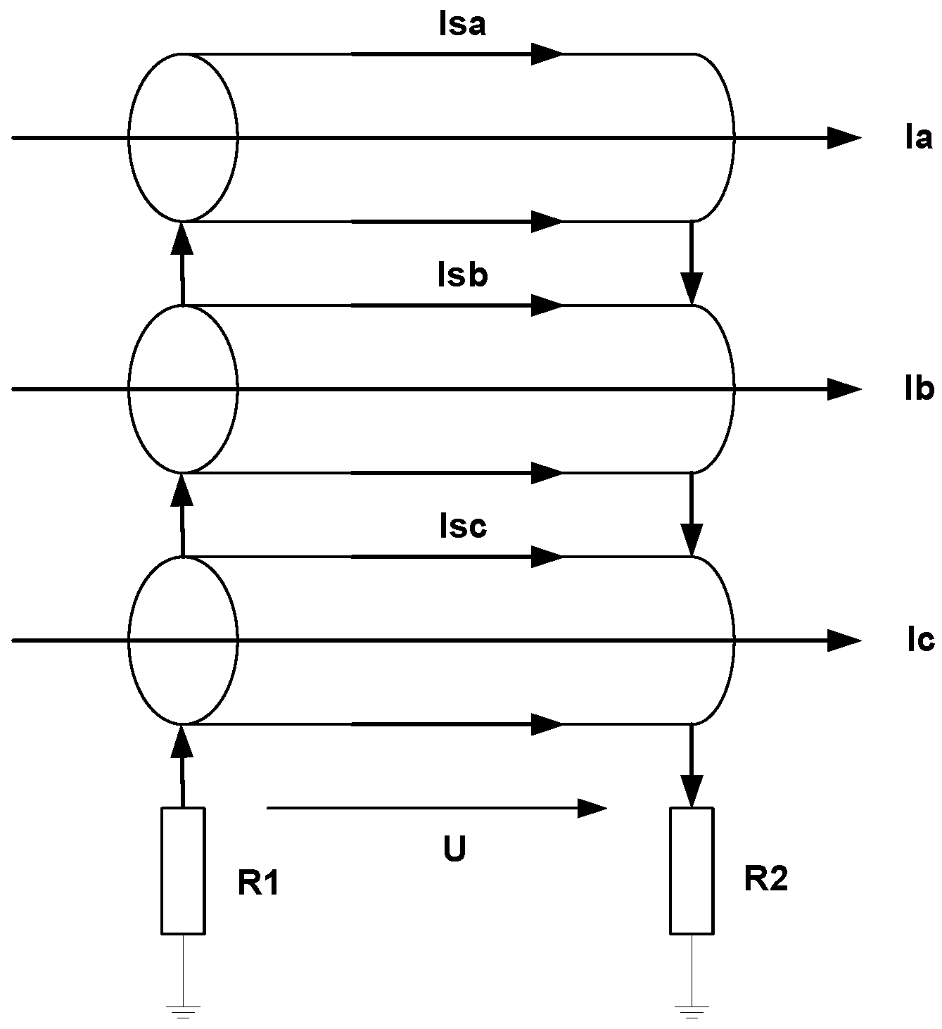
Figure 5.
Standard shields connection for SB applications. (Ia, Ib, Ic) Currents in conductors; (Isa, Isb, Isc) Currents in shields; (R1, R2) Ground resistances at both ends of shields; (U) Potential difference between shield terminals.
Figure 5.
Standard shields connection for SB applications. (Ia, Ib, Ic) Currents in conductors; (Isa, Isb, Isc) Currents in shields; (R1, R2) Ground resistances at both ends of shields; (U) Potential difference between shield terminals.
Figure 6.
Currents of the cables measured in the active conductors and their shields.
Figure 6.
Currents of the cables measured in the active conductors and their shields.
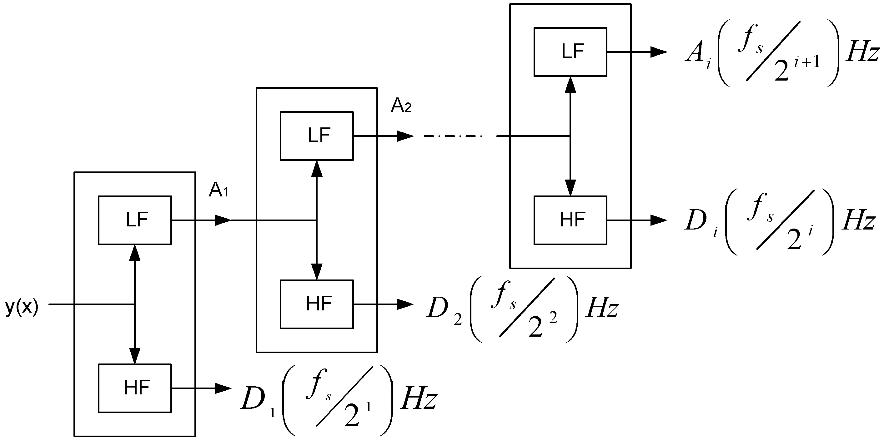
Figure 7.
Wavelet transform. Frequency bands related to decomposition steps.
Figure 7.
Wavelet transform. Frequency bands related to decomposition steps.
Figure 8.
Algorithm of the new auto-reclosing blocking method.
Figure 8.
Algorithm of the new auto-reclosing blocking method.
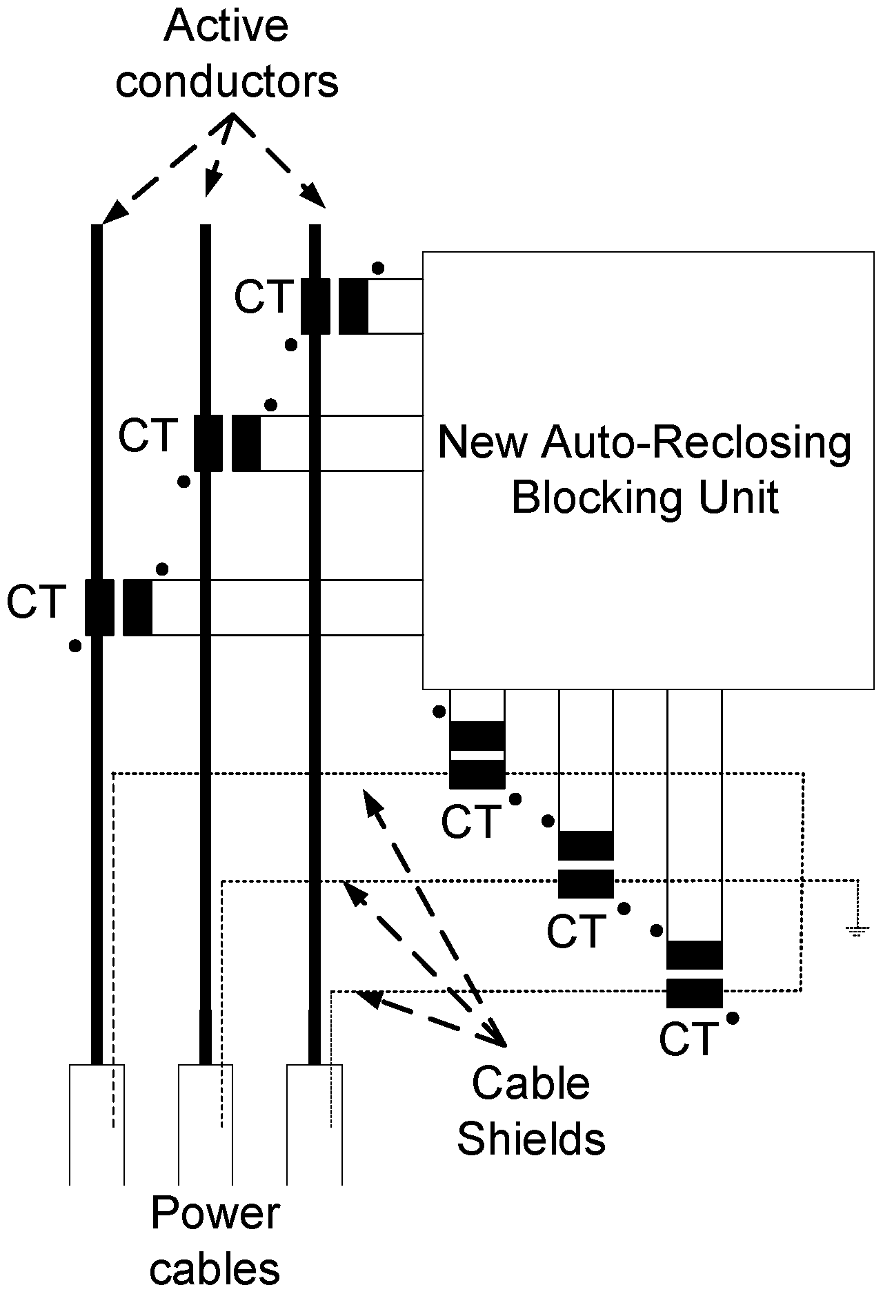
Figure 9.
New auto-reclosing blocking method: model implemented.
Figure 9.
New auto-reclosing blocking method: model implemented.
Figure 10.
Angular differences with ground fault at the overhead side in phase L1.
Figure 10.
Angular differences with ground fault at the overhead side in phase L1.
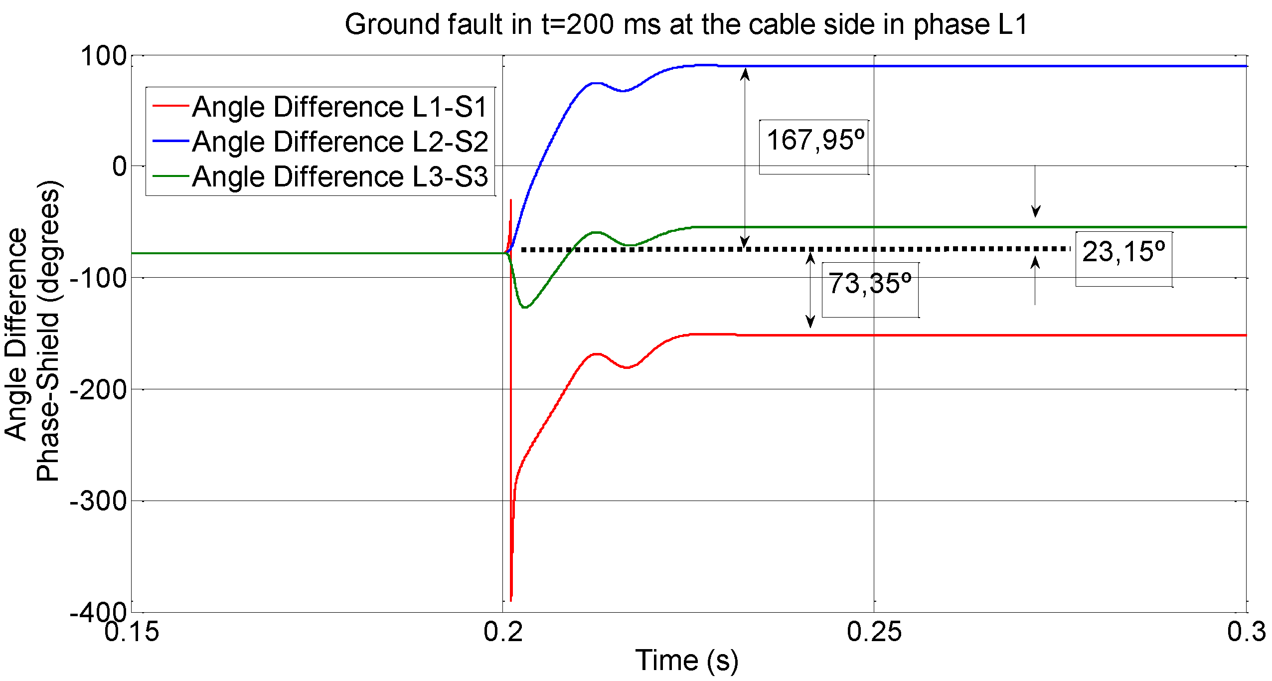
Figure 11.
Angular differences with ground fault at the cable line side in phase L1.
Figure 11.
Angular differences with ground fault at the cable line side in phase L1.
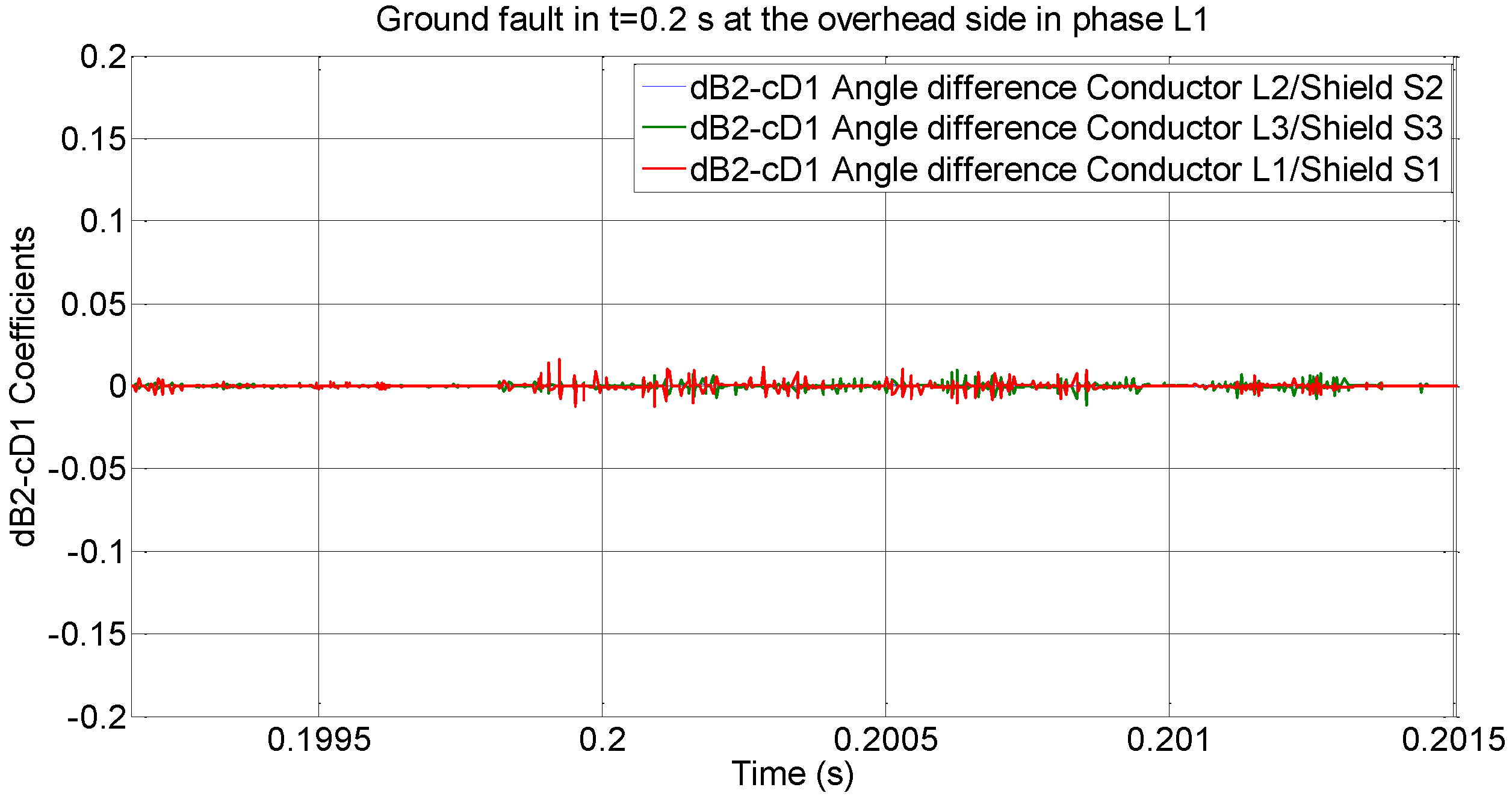
Figure 12.
Wavelet dB2-1-cD1 coefficients of the angular difference signals with ground fault in phase L1 at the overhead side 12 km from the transition.
Figure 12.
Wavelet dB2-1-cD1 coefficients of the angular difference signals with ground fault in phase L1 at the overhead side 12 km from the transition.
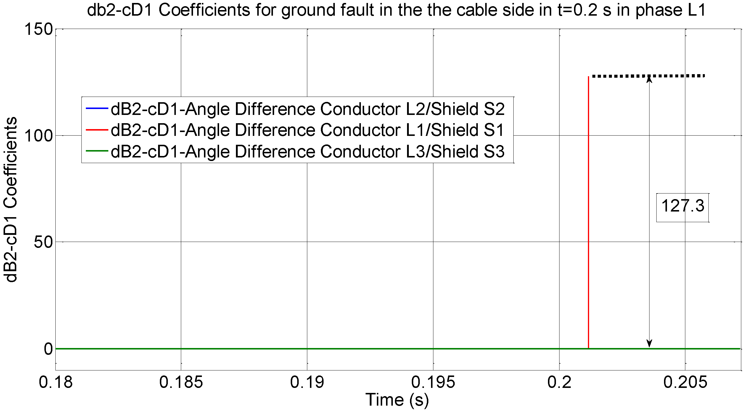
Figure 13.
Wavelet dB2-1-cD1 coefficients of the angular difference signals with ground fault in phase L1 at the cable line side 300 m from the transition.
Figure 13.
Wavelet dB2-1-cD1 coefficients of the angular difference signals with ground fault in phase L1 at the cable line side 300 m from the transition.
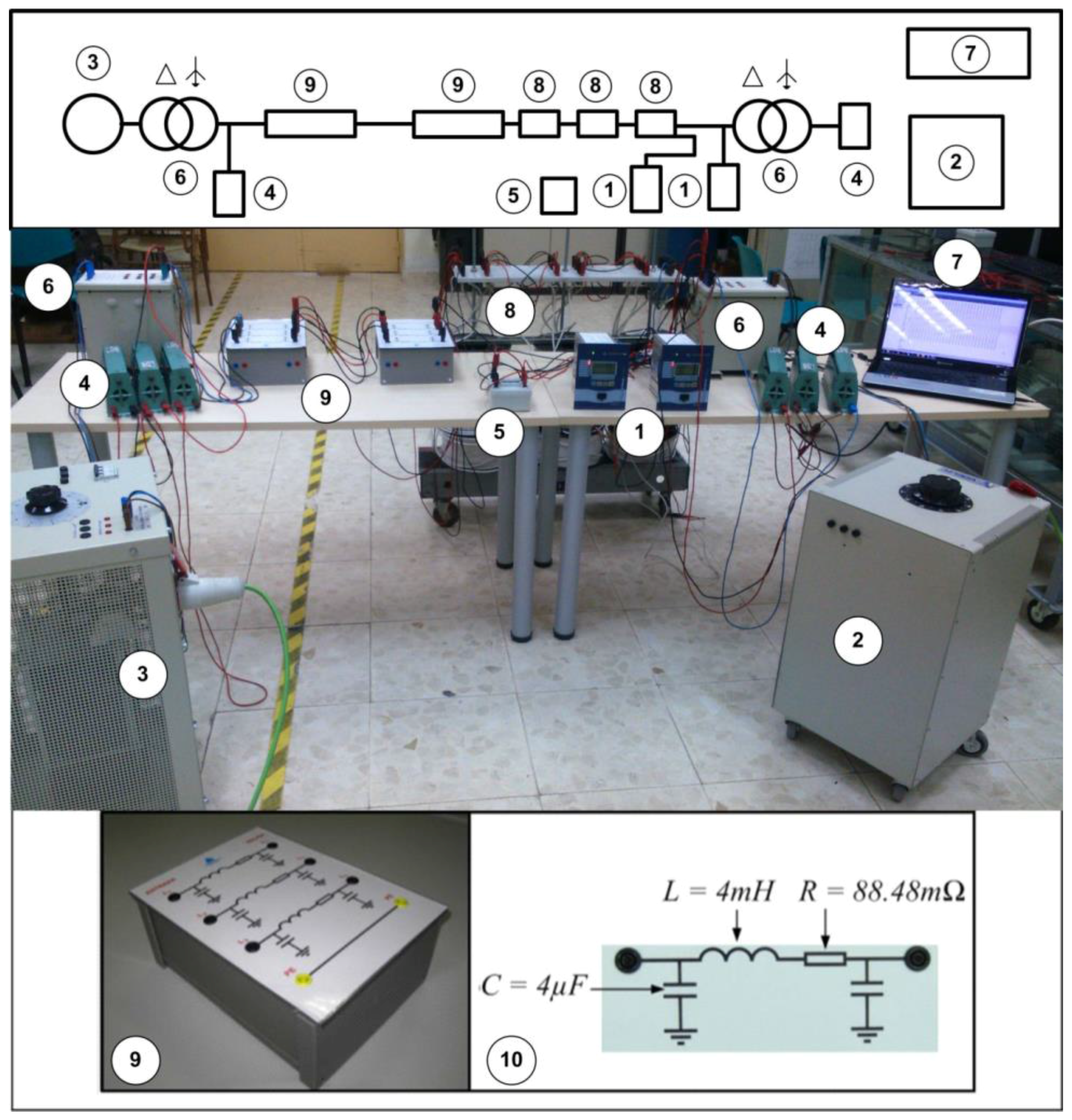
Figure 14.
Experimental setup. 1: Protection relays; 2: Auxiliary power supply; 3: Power supply; 4: Loads; 5: Ground fault switch; 6: Transformer; 7: PC; 8: Cables; 9: Line modules; 10: RLC parameters of the line modules (9) used.
Figure 14.
Experimental setup. 1: Protection relays; 2: Auxiliary power supply; 3: Power supply; 4: Loads; 5: Ground fault switch; 6: Transformer; 7: PC; 8: Cables; 9: Line modules; 10: RLC parameters of the line modules (9) used.
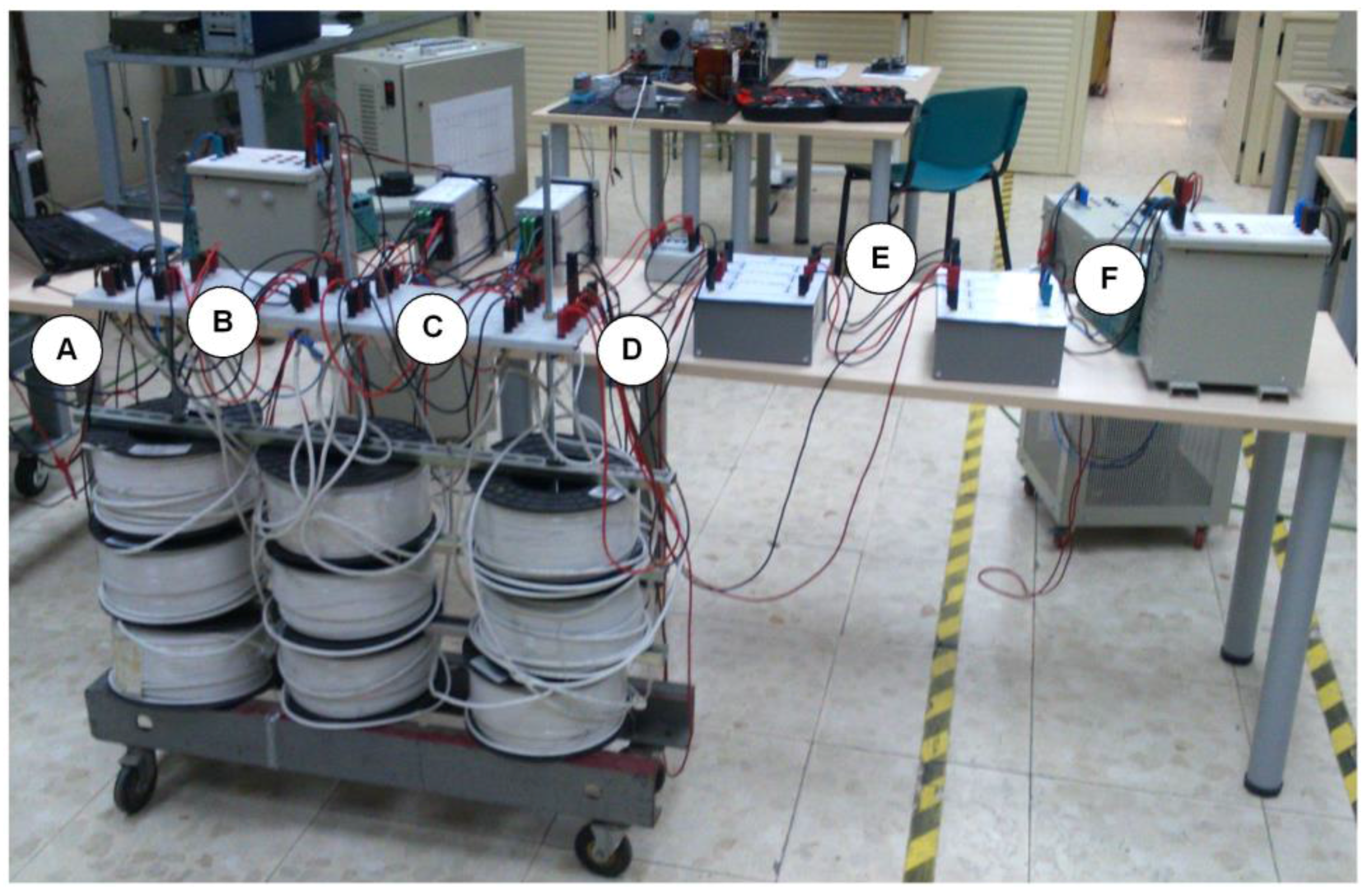
Figure 15.
Ground fault positions. A: At the end of the cable; B: Between the first and second sections of the cables; C: Between the second and third sections of the cables; D: In the transition at the end of the cables; E: Between the first and second trams of the line modules; F: Behind the two line modules.
Figure 16.
Ground fault positions: schematic representation.
Figure 16.
Ground fault positions: schematic representation.
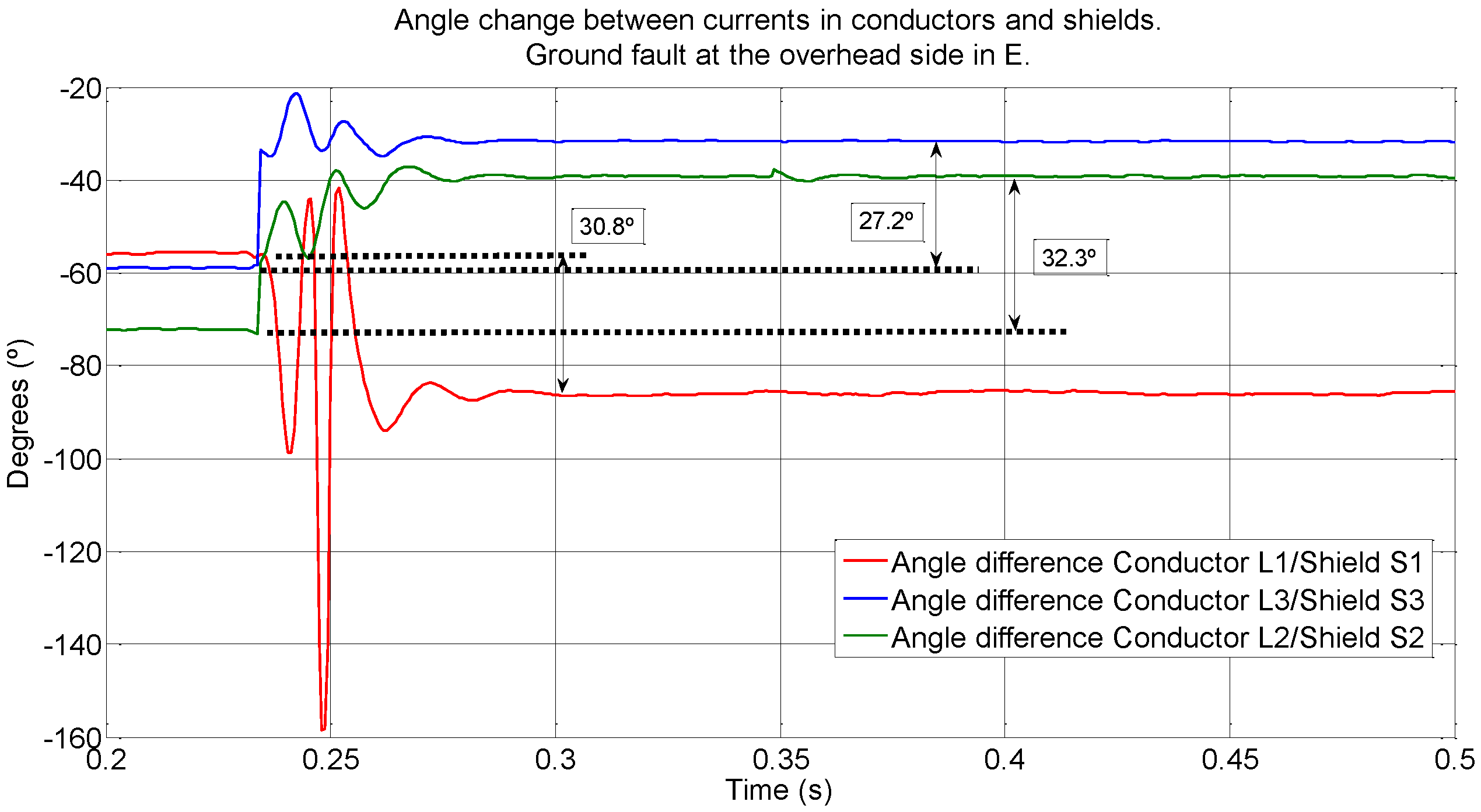
Figure 17.
Angular differences with ground fault at the overhead side in phase L1. Fault point E.
Figure 17.
Angular differences with ground fault at the overhead side in phase L1. Fault point E.
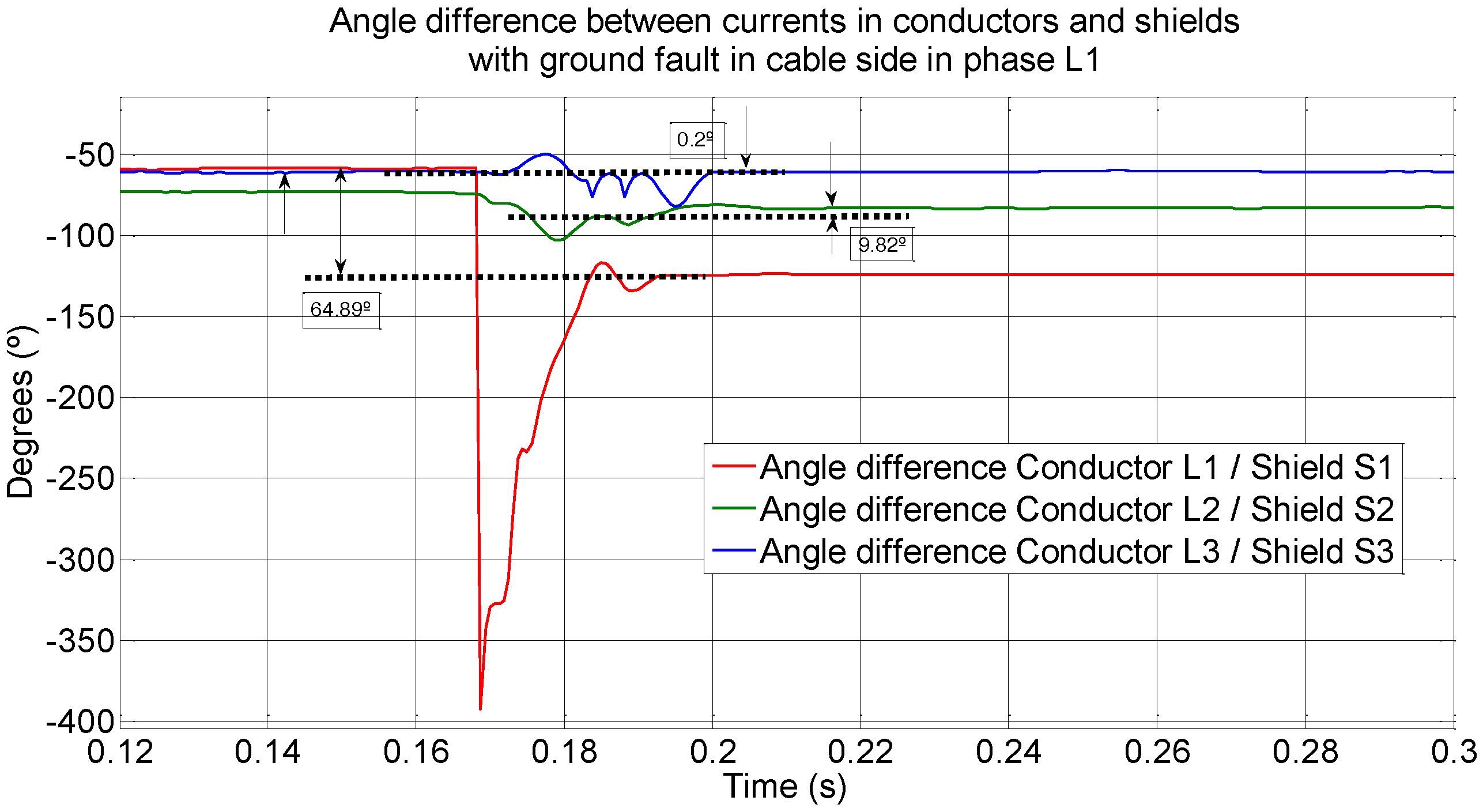
Figure 18.
Angular differences with ground fault at the cable line side in phase L1. Fault point C.
Figure 18.
Angular differences with ground fault at the cable line side in phase L1. Fault point C.
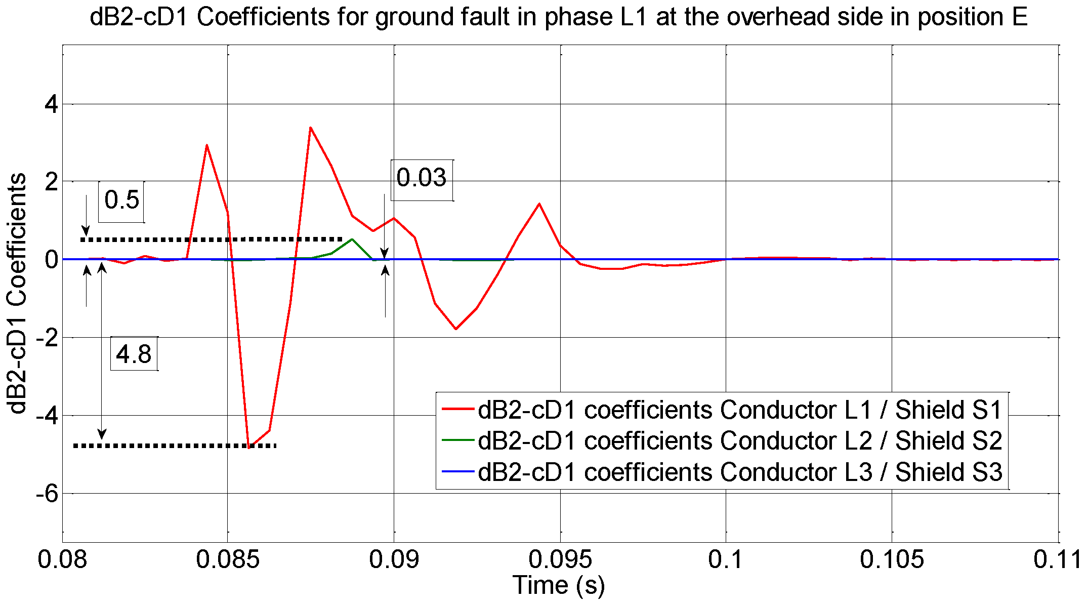
Figure 19.
Wavelet analysis of the angular differences with a ground fault at the overhead line side in phase L1. Fault point E.
Figure 19.
Wavelet analysis of the angular differences with a ground fault at the overhead line side in phase L1. Fault point E.
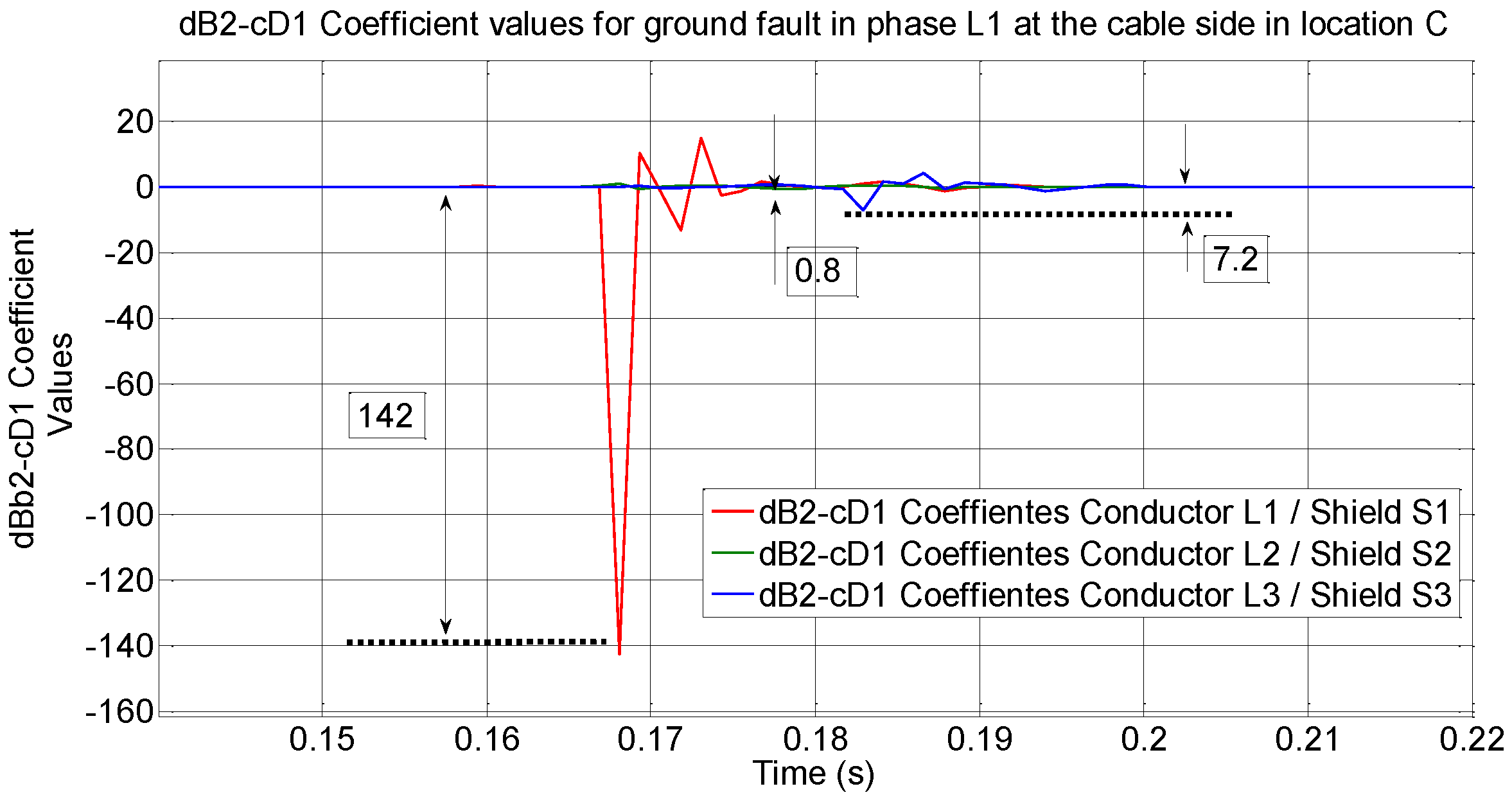
Figure 20.
Wavelet analysis of the angular differences with a ground fault at the cable line side in phase L1. Fault point C.
Figure 20.
Wavelet analysis of the angular differences with a ground fault at the cable line side in phase L1. Fault point C.
Table 1.
Phase angle variation with ground faults at the overhead and cable line sides.
Table 1.
Phase angle variation with ground faults at the overhead and cable line sides.
| Fault at Overhead Line Side | Fault at Cable Line Side |
| Distance from Transition | Fault in Phase L1 | Distance from Transition | Fault in Phase L1 |
| Variation in Phase Angles | Variation in Phase Angles |
| ΔL1S1 | ΔL2S2 | ΔL3S3 | ΔL1S1 | ΔL2S2 | ΔL3S3 |
| 1 m | 15.18° | 10.98° | 15.26° | 1 m | 73.69° | 168.62° | 24.03° |
| 10 m | 15.16° | 10.99° | 15.24° | 10 m | 73.72° | 168.65° | 24.05° |
| 100 m | 15.17° | 11.01° | 15.26° | 50 m | 73.75° | 168.61° | 24.12° |
| 1000 m | 15.18° | 11.05° | 14.27° | 100 m | 73.71° | 168.52° | 23.73° |
| 5000 m | 15.25° | 11.33° | 15.37° | 300 m | 73.35° | 167.95° | 23.15° |
| >10,000 m | 15.44° | 12.20° | 15.64° | 599 m | 67.32° | 157.11° | 27.67° |
| Fault at Overhead Line Side | Fault at Cable Line Side |
| Distance from Transition | Fault in Phase L2 | Distance from Transition | Fault in Phase L2 |
| Variation in Phase Angles | Variation in Phase Angles |
| ΔL1S1 | ΔL2S2 | ΔL3S3 | ΔL1S1 | ΔL2S2 | ΔL3S3 |
| 1 m | 15.34° | 15.33° | 10.81° | 1 m | 24.02° | 73.72° | 168.58° |
| 10 m | 15.35° | 15.34° | 10.88° | 10 m | 24.10° | 73.70° | 168.59° |
| 100 m | 15.34° | 15.33° | 10.87° | 50 m | 23.92° | 73.71° | 168.47° |
| 1000 m | 15.37° | 15.36° | 10.85° | 100 m | 23.85° | 73.79° | 168.42° |
| 5000 m | 15.48° | 15.45° | 11.20° | 300 m | 22.99° | 73.55° | 167.65° |
| >10,000 m | 15.67° | 15.56° | 11.72° | 599 m | 27.87° | 67.51° | 157.52° |
| Fault at Overhead Line Side | Fault at Cable Line Side |
| Distance from Transition | Fault in Phase L3 | Distance from transition | Fault in Phase L3 |
| Variation in Phase Angles | Variation in Phase Angles |
| ΔL1S1 | ΔL2S2 | ΔL3S3 | ΔL1S1 | ΔL2S2 | ΔL3S3 |
| 1 m | 11.78° | 15.41° | 15.25° | 1 m | 168.61° | 24.01° | 73.31° |
| 10 m | 11.79° | 15.42° | 15.22° | 10 m | 168.62° | 24.02° | 73.70° |
| 100 m | 11.77° | 15.43° | 15.23° | 50 m | 168.51° | 23.92 | 73.72° |
| 1000 m | 11.82° | 15.45° | 15.25° | 100 m | 168.40° | 23.75° | 73.31° |
| 5000 m | 12.13° | 15.55° | 15.33° | 300 m | 168.12° | 23.11° | 73.55° |
| >10,000 m | 12.66° | 15.73° | 15.45° | 599 m | 157.36° | 67.78° | 68.01° |
Table 2.
Wavelet analysis: simulation results. Ground faults at the overhead and cable line sides. Overhead line side solidly grounded and cable line side isolated. Phase currents measured in the conductors (L1, L2, L3) and in their shields (S1, S2, S3).
Table 2.
Wavelet analysis: simulation results. Ground faults at the overhead and cable line sides. Overhead line side solidly grounded and cable line side isolated. Phase currents measured in the conductors (L1, L2, L3) and in their shields (S1, S2, S3).
| Fault at Overhead Line Side | Fault at Cable Line Side |
| Distance from Transition | Fault in Phase L1 | Distance from Transition | Fault in Phase L1 |
| W (dB2-cD1 Coefficients) | W (dB2-cD1 Coefficients) |
| ΔL1S1 | ΔL2S2 | ΔL3S3 | ΔL1S1 | ΔL2S2 | ΔL3S3 |
| 1 m | 0.0068 | 0.0067 | 0.0065 | 1 m | 173.88 | 0.0134 | 0.0096 |
| 10 m | 0.0039 | 0.0041 | 0.0041 | 10 m | 173.89 | 0.0123 | 0.0097 |
| 100 m | 0.0033 | 0.0038 | 0.0039 | 50 m | 127.32 | 0.0113 | 0.0094 |
| 1000 m | 0.0027 | 0.0029 | 0.0025 | 100 m | 127.32 | 0.0119 | 0.0097 |
| 5000 m | 0.0019 | 0.0024 | 0.0019 | 300 m | 127.31 | 0.0128 | 0.0089 |
| >10,000 m | 0.0014 | 0.0016 | 0.0013 | 599 m | 123.67 | 0.02784 | 0.0332 |
| Fault at Overhead Line Side | Fault at Cable Line Side |
| Distance from Transition | Fault in Phase L2 | Distance from Transition | Fault in Phase L2 |
| W (dB2-cD1 Coefficients) | W (dB2-cD1 Coefficients) |
| ΔL1S1 | ΔL2S2 | ΔL3S3 | ΔL1S1 | ΔL2S2 | ΔL3S3 |
| 1 m | 0.0067 | 0.0064 | 0.0069 | 1 m | 0.0095 | 173.90 | 0.0136 |
| 10 m | 0.0044 | 0.0039 | 0.0042 | 10 m | 0.0098 | 173.90 | 0.0122 |
| 100 m | 0.0037 | 0.0031 | 0.0039 | 50 m | 0.0095 | 127.30 | 0.0114 |
| 1000 m | 0.0029 | 0.0022 | 0.0028 | 100 m | 0.0098 | 127.30 | 0.0120 |
| 5000 m | 0.0021 | 0.0017 | 0.0022 | 300 m | 0.0088 | 127.31 | 0.0130 |
| >10,000 m | 0.0016 | 0.0011 | 0.0015 | 599 m | 0.0333 | 123.70 | 0.02782 |
| Fault at Overhead Line Side | Fault at Cable Line Side |
| Distance from Transition | Fault in Phase L3 | Distance from Transition | Fault in Phase L3 |
| W (dB2-cD1 Coefficients) | W (dB2-cD1 Coefficients) |
| ΔL1S1 | ΔL2S2 | ΔL3S3 | ΔL1S1 | ΔL2S2 | ΔL3S3 |
| 1 m | 0.0066 | 0.0064 | 0.0065 | 1 m | 0.0135 | 0.0094 | 173.91 |
| 10 m | 0.0044 | 0.0045 | 0.0037 | 10 m | 0.0121 | 0.0097 | 173.91 |
| 100 m | 0.0037 | 0.0039 | 0.0030 | 50 m | 0.0113 | 0.0097 | 127.29 |
| 1000 m | 0.0029 | 0.0031 | 0.0024 | 100 m | 0.0121 | 0.0099 | 127.29 |
| 5000 m | 0.0023 | 0.0023 | 0.0018 | 300 m | 0.0131 | 0.0087 | 127.30 |
| >10,000 m | 0.0016 | 0.0015 | 0.0013 | 599 m | 0.02783 | 0.0334 | 127.71 |
Table 3.
Ground fault at overhead and cable line sides in phase L1. Variation in phase angles between currents in the conductors and their respective shields.
Table 3.
Ground fault at overhead and cable line sides in phase L1. Variation in phase angles between currents in the conductors and their respective shields.
| Fault at Cable Line Side |
| Place of the Fault | Fault in Phase L1 |
| Variation in Phase Angles |
| ΔL1S1 | ΔL2S2 | ΔL3S3 |
| A | 66.32° | 11.02° | 0.33° |
| B | 65.93° | 10.24° | 0.26° |
| C | 64.89° | 9.82° | 0.20° |
| D | 64.25° | 9.31° | 0.18° |
| Fault at Overhead Line Side |
| Place of the Fault | Fault in Phase L1 |
| Variation in Phase Angles |
| ΔL1S1 | ΔL2S2 | ΔL3S3 |
| E | 30.80° | 32.31° | 27.16° |
| F | 29.12° | 31.86° | 26.02° |
Table 4.
Ground fault at overhead and cable line sides in phase L2. Variation in phase angles between currents in the conductors and their respective shields.
Table 4.
Ground fault at overhead and cable line sides in phase L2. Variation in phase angles between currents in the conductors and their respective shields.
| Fault at Cable Line Side |
| Place of the Fault | Fault in Phase L2 |
| Variation in Phase Angles |
| ΔL1S1 | ΔL2S2 | ΔL3S3 |
| A | 0.29° | 66.45° | 12.08° |
| B | 0.25° | 65.99° | 10.93° |
| C | 0.21° | 65.02° | 9.88° |
| D | 0.16° | 64.67° | 9.33° |
| Fault at Overhead Line Side |
| Place of the Fault | Fault in Phase L2 |
| Variation in Phase Angles |
| ΔL1S1 | ΔL2S2 | ΔL3S3 |
| E | 1.29° | 31.78° | 16.29° |
| F | 1.11° | 25.11° | 12.11° |
Table 5.
Ground fault at overhead and cable line sides in phase L3. Variation in phase angles between currents in the conductors and their respective shields.
Table 5.
Ground fault at overhead and cable line sides in phase L3. Variation in phase angles between currents in the conductors and their respective shields.
| Fault at Cable Line Side |
| Place of the Fault | Fault in Phase L3 |
| Variation in Phase Angles |
| ΔL1S1 | ΔL2S2 | ΔL3S3 |
| A | 12.58° | 0.30° | 67.34° |
| B | 10.13° | 0.26° | 66.86° |
| C | 9.01° | 0.20° | 65.78° |
| D | 8.92° | 0.18° | 64.02° |
| Fault at Overhead Line Side |
| Place of the Fault | Fault in Phase L3 |
| Variation in Phase Angles |
| ΔL1S1 | ΔL2S2 | ΔL3S3 |
| E | 17.34° | 1.35° | 32.45° |
| F | 14.22° | 1.18° | 23.67° |
Table 6.
Ground fault at overhead and cable line sides. Wavelet analysis: experimental results. Overhead line side solidly grounded and cable line side isolated.
Table 6.
Ground fault at overhead and cable line sides. Wavelet analysis: experimental results. Overhead line side solidly grounded and cable line side isolated.
| Fault at Cable Line Side | Fault at Overhead Line Side |
| Location of the Fault | Fault in Phase L1 | Location of the Fault | Fault in Phase L1 |
| W (dB2-cD1 Coefficients) | W (dB2-cD1 Coefficients) |
| ΔL1S1 | ΔL2S2 | ΔL3S3 | ΔL1S1 | ΔL2S2 | ΔL3S3 |
| A | 152.24 | 2.45 | 18.29 | E | 4.80 | 0.03 | 0.50 |
| B | 145.88 | 1.96 | 14.12 |
| C | 142.01 | 0.80 | 7.21 | F | 4.66 | 0.02 | 0.42 |
| D | 136.54 | 0.69 | 4.75 |
| Fault at Cable Line Side | Fault at Overhead Line Side |
| Location of the Fault | Fault in Phase L2 | Location of the Fault | Fault in Phase L2 |
| W (dB2-cD1 Coefficients) | W (dB2-cD1 Coefficients) |
| ΔL1S1 | ΔL2S2 | ΔL3S3 | ΔL1S1 | ΔL2S2 | ΔL3S3 |
| A | 20.04 | 154.31 | 3.01 | E | 0.04 | 4.88 | 0.59 |
| B | 16.59 | 148.22 | 2.42 |
| C | 9.92 | 143.67 | 0.89 | F | 0.03 | 4.72 | 0.48 |
| D | 6.82 | 138.08 | 0.82 |
| Fault at Cable Line Side | Fault at Overhead Line Side |
| Location of the Fault | Fault in Phase L3 | Location of the Fault | Fault in Phase L3 |
| W (dB2-cD1 Coefficients) | W (dB2-cD1 Coefficients) |
| ΔL1S1 | ΔL2S2 | ΔL3S3 | ΔL1S1 | ΔL2S2 | ΔL3S3 |
| A | 2.66 | 19.44 | 153.01 | E | 0.47 | 0.04 | 4.34 |
| B | 1.49 | 15.18 | 144.78 |
| C | 0.81 | 6.96 | 140.12 | F | 0.51 | 0.02 | 4.11 |
| D | 0.52 | 3.97 | 134.96 |


 ,
, 


