Analysis of Power Quality Signals Using an Adaptive Time-Frequency Distribution

Abstract

Spikes frequently occur in power quality (PQ) disturbance signals due to various causes such as switching of the inductive loads and the energization of the capacitor bank. Such signals are difficult to analyze using existing time-frequency (TF) methods as these signals have two orthogonal directions in a TF plane. To address this issue, this paper proposes an adaptive TF distribution (TFD) for the analysis of PQ signals. In the proposed adaptive method, the smoothing kernel’s direction is locally adapted based on the direction of energy in the joint TF domain, and hence an improved TF resolution can be obtained. Furthermore, the performance of the proposed adaptive technique in analyzing electrical PQ is thoroughly studied for both synthetic and real world electrical power signals with the help of extensive simulations. The simulation results (specially for empirical data) indicate that the adaptive TFD method achieves high energy concentration in the TF domain for signals composed of tones and spikes. Moreover, the local adaptation of the smoothing kernel in the adaptive TFD enables the extraction of TF signature of spikes from TF images, which further helps in measuring the energy of spikes in a given signal. This new measure can be used to both detect the spikes as well as to quantify the extent of distortion caused by the spikes in a given signal.

1. Introduction

Electric power quality (PQ) is a broad term which covers various aspects in the areas concerning electrical power transmission to its distribution to consumers. Different types of PQ issues are usually encountered in power systems including the voltage sag, swell, harmonics and transients. All of these PQ issues arise due to the non-linear behavior of load on the transmission distribution system. These disturbing loads cause a deviation in the voltage and current waveforms which lead to significant degradation in the performance of power systems. In addition, there are multiple sources of different PQ disturbances appearing simultaneously, thus making it a challenging task to detect them individually. PQ also affects the performances of end user equipment, which is connected to the power system. Due to such degradation in the performance of electric power systems, PQ has become a major area of concern for utility companies. In order to improve the PQ, utilities must first record the information about the statistical behavior of the voltage and current in a power system and subsequently analyze that information for the occurrence of disturbances in order to avoid any damage to the equipment. These requirements have sparked a lot of interest in the development of signal processing algorithms for the analysis of electrical PQ [1,2,3,4,5,6,7,8,9].

Due to non-stationary characteristics of power signals, time-frequency (TF) signal processing techniques are preferred tools for both analysis and the automated classification of these signals [10]. TF signal analysis methods can be broadly categorized into linear methods and quadratic methods [10]. Linear methods such as short time-Fourier transform are simple to implement, but suffer from low resolution [10]. Quadratic TF methods, on the other hand, offer relatively higher TF resolution as compared to the linear TF methods. The Wigner–Ville distribution (WVD) is the underlying TF distribution (TFD) for all quadratic TFDs. It provides ideal energy concentration for mono-component signals but suffers from cross-term interference for multi-component signals [11]. The effects of cross-terms can be reduced by employing a two-dimensional (2D) smoothing kernel, but this also degrades the energy concentration of auto-terms [12]. Another alternative method for reducing cross-terms in the WVD is to compute the Gabor Wigner transform, which is defined as the multiplication of Gabor transform with the WVD [13]. This Gabor Wigner transform provides the combined advantages of both the WVD and short time-Fourier transform, by offering high energy concentration of auto-terms and by also removing cross-terms.

Spikes/transients are frequently observed in electrical PQ signals. They are caused by the switching of high inductive loads, and are due to capacitor bank energization [14]. When an electric spike occurs, a high surge of voltage/current passes through electric equipment and can cause damage to electric appliances. Specifically, transients/spikes can cause electrical devices to operate erratically, such as micro-jogging in motors, and it may also lead to a failure of the lighting equipment. Therefore, it is imperative to detect these power quality issues [15,16,17,18].

Multi-resolution signal analysis methods such as the S-transform and the Hilbert transform are also commonly used for the analysis and classification of PQ signals [19,20,21]. S-transform is particularly useful for the analysis of signals with spikes as the shape of its analysis window is frequency dependent. It provides high energy concentration for signals composed of spikes and low frequency content. The Hilbert–Huang transform is also an effective tool for the analysis of non-stationary signals [22]. However, it is only suitable for signals that can be modelled as amplitude modulated and frequency modulated signals.

Recently, an adaptive time frequency based method (ADTFD) has been proposed which adapts the direction of smoothing kernel locally on a point-by-point basis for the analysis and the parameter estimation of frequency modulated signals [23,24]. This method outperforms other TFDs in terms of its ability to resolve closely placed signal components, and has found applications in areas such as pattern recognition, direction of arrival estimation and signal classification [25,26]. The ADTFD method, however, focuses mainly on the analysis of non-stationary frequency modulated signals. For such signals, the direction of smoothing kernel can be from the set of all possible directions (covering the whole range of θ) in the TF plane. In this work, our focus has been on the PQ disturbance signals where spikes and sinusoids are the main disturbances. Therefore, we have modified the method given in [23,24] so that it could be effectively used for the detection of spikes in the PQ signals. This is achieved by limiting the directions of the smoothing kernel to only two angles, $\theta =0$ and $\theta =90$ degrees, which correspond to the horizontal and vertical axes of the TF plane where sinusoids and spikes reside, respectively. The performance of the proposed method is compared against the state of the art TF based methods in terms of its ability to analyse PQ signals. Finally, a new metric is presented which can be used to separate the signature of spikes from that of the tones in the PQ signals.

The rest of this paper is organized as follows: signal model for the PQ signals is described in Section 2. Section 3 presents a review of the commonly used time-frequency methods and discusses the drawbacks of these methods for analyzing PQ signals. Section 4 discusses the proposed adaptive TFD method in consideration of the analysis of the PQ signals. A detailed numerical analysis considering both synthetic and real world electrical signals is presented in Section 5. Finally, concluding remarks on the proposed technique and the obtained simulation results are presented in Section 6.

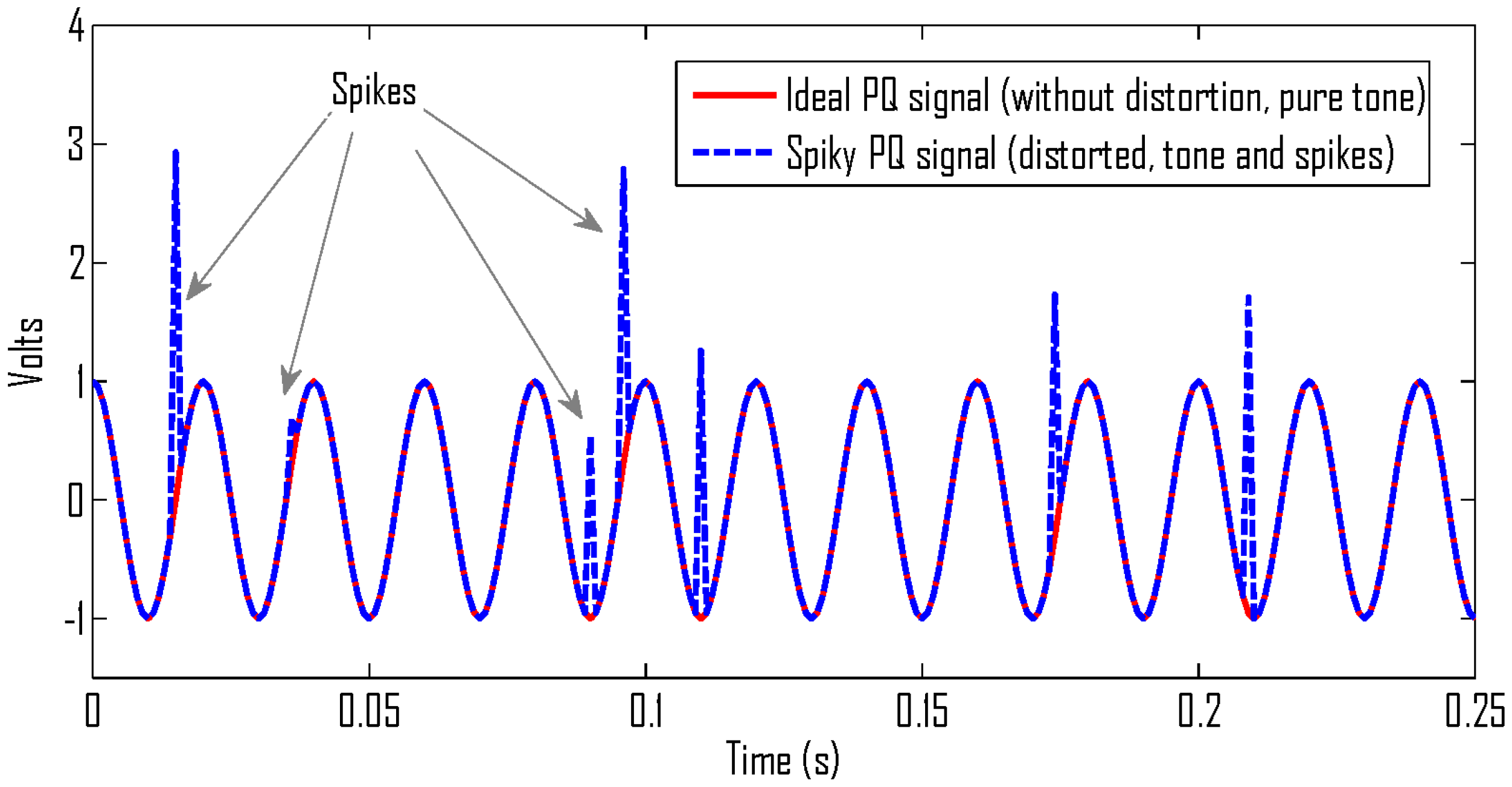
2. Signal Model for Power Quality Signals

A PQ signal without any distortion is a pure tone (i.e., sinusoid), which can be expressed as

$$x(t)=\cos (2\pi f_{0}t),$$

(1)

where $f_0$ is the fundamental frequency of a signal. The PQ signals are sometimes corrupted by the harmonics related to the fundamental frequency and can be represented as

$$x(t)=\sum _{k=1}^N\cos (2\pi k{f}_{0}t).$$

(2)

In some cases, a PQ signal is corrupted by sudden transients or spikes. Therefore, a more general model of PQ can be written as

$$x(t)=\sum _{k=1}^N\cos (2\pi k{f}_{0}t)+\sum _{k=1}^M\delta (t-T_k),$$

(3)

where $\delta (t-T_k)$ is an impulse shifted at $T_k$ seconds in time. One such PQ signal obtained by the combination of tones and impulses is illustrated in Figure 1.

3. Review of Time-Frequency Distributions

3.1. Quadratic Time-Frequency Distributions

The WVD is a core distribution of the quadratic class of TFDs. It can be obtained by taking Fourier transform of the instantaneous auto-correlation function in the following way [12]:

$$W_z(t,f)=\int w(\tau )z(t+\frac{\tau }{2})z^{*}(t-\frac{\tau }{2})e^{-j2\pi f\tau },\mathrm{d}\tau ,$$

(4)

where $w(\tau )$ is a time lag window, $z(t)$ is the analytic associate of a real signal $s(t)$, and $W_z(t,f)$ is the WVD. The problem with the WVD is that it suffers from cross-term interference for multi-component signals due to its quadratic nature [12]. Cross-terms have oscillatory characteristics and the rate of oscillation depends on the distance between two auto-terms [11]. The cross-terms of the WVD are suppressed by employing a 2D smoothing kernel [12]. All TFDs belonging to the quadratic class, including the Spectrogram, can be obtained by smoothing the WVD as follows:

$$\rho \left(t,f\right)=\gamma \left(t,f\right)\hspace{0.17em}\underset{\left(t,f\right)}{**}\hspace{0.17em}{W}_z\left(t,f\right),$$

(5)

where $\rho \left(t,f\right)$ is a quadratic TFD, $\gamma \left(t,f\right)$ is a 2D smoothing filter, and $\underset{\left(t,f\right)}{**}$ represents 2D convolution along time and frequency axes.

Quadratic TFDs suffer from inherent compromise between suppression of cross-terms and the energy concentration of auto-terms. Intensive smoothing results in almost complete removal of cross-terms, e.g., in the case of Spectrogram. However, such smoothing results in blurring of auto-terms, thus affecting the resolution capability of a quadratic TFD. Previous studies have shown that separable kernel TFDs, i.e., TFDs whose smoothing kernel can be represented as the product of two smoothing functions: $\gamma \left(t,f\right)=g(t)G(f)$, offer better compromise in cross-term suppression and auto-term preservation [12]. This gain is achieved due to the flexibility of independently adjusting the smoothing along time and frequency axes, which is not available in the case of the commonly used Spectrogram [12].

3.2. Linear Short Time Fourier Transform

One alternative to the quadratic class of TFDs is linear time-frequency representations. One popular distribution of this class is short time-Fourier transform and is defined as:

$$STFT(t,f)=\int w(\tau )z(t+\tau )e^{-j2\pi f\tau }\mathrm{d}\tau ,$$

(6)

where $w(\tau )$ is an analysis window. The short time-Fourier transform is a linear method. Hence, it does not suffer from the cross-term interference problem commonly observed in quadratic methods. The performance of this transform depends on the selection of an analysis window [10]. A wide window offers good resolution along the frequency axis but poor resolution along the time axis, while a narrow window provides good resolution along the time axis and poor resolution along the frequency axis [10]. This limitation can be overcome to an extent by using the wavelet transform [10], which offers high resolution along time and frequency axes for higher and lower frequencies, respectively. However, the performance of the wavelet transform also depends on the selection of mother wavelets that need to be optimized manually for each signal to obtain an optimal performance.

In the case of power quality disturbance signals, we can have both spikes and tones in single composite signals. For such signals, it is impossible to select a single window that achieves high energy concentration for both spikes and tones. A short window would result in good energy concentration of the spikes but would deteriorate the energy concentration of the tones and vice versa.

3.3. Gabor Wigner Transform: A Combination of Linear and Quadratic Methods

The short time-Fourier transform does not suffer from the cross-term interference problem but suffers from poor energy concentration of auto-terms. On the other hand, the WVD offers high energy concentration of auto-terms but suffers from the cross-term interference problem. One way to combine the advantages of linear and quadratic time-frequency methods, i.e., to obtain a TFD with a high energy concentration of auto-terms with the elimination of cross-terms is to simply multiply a short time-Fourier transform with the WVD [13]. The TFD obtained as a multiplication of short time-Fourier transform and WVD is called the Gabor Wigner transform (GWT) and is defined as [13]:

$$GWT\left(t,f\right)=GT\left(t,f\right)\hspace{0.17em}{W}_z\left(t,f\right),$$

(7)

where $GT\left(t,f\right)$ is simply a short time-Fourier transform with a Gaussian window. The GWT has emerged as a powerful tool for the analysis of a number of real-life signals due to its ability to achieve high energy concentration of auto-terms with significant cross-term suppression including power quality disturbance signals [8,27].

The Gabor Wigner transform, however, fails to achieve optimal energy concentration in the situations when auto-terms overlap with cross-terms [28,29]. Such a situation emerges when signal components have very close components that ordinary short time Fourier transform fails to resolve. In the case of PQ signals, such a situation appears when a given signal is corrupted by a train of closely spaced spikes.

4. Proposed Methodology

This section presents the proposed method for the analysis of power quality signals.

4.1. Adaptive TFD for PQ Signals

An adaptive time frequency distribution for the analysis of power quality signals is presented in this subsection. This method suppresses the interference terms of the WVD using adaptive directional smoothing. Note that any quadratic TFD can be selected for the adaptive method, but we have selected the WVD due its high resolution. Furthermore, this method exploits the fact that aligning the smoothing kernel in parallel to the direction of auto-terms can lead to a high resolution TF representation [30]. Such TFDs with the directional smoothing kernels can be expressed as [30]:

$$\rho \left(t,f\right)={\gamma }_{\theta }\left(t,f\right)\hspace{0.17em}\underset{\left(t,f\right)}{**}\hspace{0.17em}{W}_z\left(t,f\right),$$

(8)

where ${\gamma }_{\theta }$ is a kernel whose direction depends on angle θ. Such TFDs achieve good performance for signals having one direction of energy distribution in the TF domain [30]. This global alignment of the smoothing kernel is not possible for the PQ spike signals as they can have two orthogonal directions: one parallel to the time axis due to sinusoidal nature of power signals and the other parallel to the frequency axis due to spikes. For such signals, the smoothing kernel’s direction should be adapted locally as [24]:

$$\rho \left(t,f\right)={\gamma }_{\theta \left(t,f\right)}\left(t,f\right)\hspace{0.17em}\underset{\left(t,f\right)}{**}\hspace{0.17em}{W}_z,\left(t,f\right),$$

(9)

where $\theta \left(t,f\right)$ denotes the direction angles that have been adapted locally based on the input signal characteristics. In general, the PQ signals are usually modeled either as the summation of pure tones or the summation of tones and spikes. Therefore, the cross-terms appearing in the WVD of PQ signals possess the following characteristics:

• Cross-terms appear as ridges in the joint TF domain with their major axis being parallel to the direction of their oscillation [12].
• The direction of cross-terms’ oscillation, caused by the interaction of tones (fundamental frequency) and harmonics, is parallel to the time axis.
• The direction of cross-terms’ oscillation, caused by the interaction of spikes, is parallel to the frequency axis.

Note that the last two observations can be deduced from the established mathematical fact that the direction of cross-terms’ oscillation is orthogonal to the direction of a line joining components [11]. These observations indicate that the smoothing kernel should be adapted along the following two directions: (1) along the direction parallel to the time axis to suppress the cross-terms appearing due to tones; (2) along the direction parallel to the frequency axis to suppress cross-terms appearing due to spikes. This implies that the smoothing kernel should be aligned locally with the cross-terms’ major-axis at each TF point, which is the same direction as of the cross-terms’ oscillation. If we use the absolute value of a WVD, the oscillatory characteristics of the cross-terms are removed. Then, the smoothing kernel’s direction for each point in the TF plane is obtained by maximizing its correlation with the absolute value of the WVD as follows [24]:

$$\theta (t,f)=arg\underset{\theta }{max}\left||W_z(t,f)|\hspace{0.17em}\underset{\left(t,f\right)}{**}\hspace{0.17em}{\gamma }_{\theta }(t,f)\right|.$$

(10)

The above equation needs to be optimized only for two values of θ that are $\theta =0$ and $\theta =\pi /2$ as the cross-terms are either parallel to the frequency or the time axis. Once $\theta (t,f)$ is estimated, we can obtain the adaptive TFD using (9).

For the selection of the smoothing kernel, we use double derivative directional Gaussian kernel in this study, which is defined as:

$${\gamma }_{\theta \left(t,f\right)}\left(t,f\right)=\frac{ab}{2\pi }\frac{d^2}{d{f}_{\theta }^2}{e}^{-a^2{t}_{\theta }^2-b^2{f}_{\theta }^2},$$

(11)

where $t_{\theta }=tcos(\theta )+fsin(\theta )$, $f_{\theta }=-tsin(\theta )+fcos(\theta )$, θ is the rotation angle with respect to the time axis, and ${\gamma }_{\theta \left(t,f\right)}\left(t,f\right)$ is the directional Gaussian filter. The parameter a controls the smoothing of the filter along the major axis while parameter b controls the smoothing along the minor axis. Usually, a is assigned a small value to have extensive smoothing along the major axis of cross-terms and b is assigned a large value to have less intensive smoothing along the minor axis to avoid the merging of close signal components [24]. Further details regarding the automatic optimization of parameters can be found in [23]. The main features of the employed kernel are highlighted below:

• It has a low pass characteristic response when it is aligned parallel to ridges, that is, along the major axis of auto- or cross-terms. This low pass characteristic results in the reduction of cross-terms and signal to noise ratio enhancement of auto-terms.
• The response of this kernel becomes zero when it becomes orthogonal to the major axis of auto-terms. This characteristic of the smoothing kernel avoids the spreading of signal energy for TF points where no signal is present.

4.2. Feature Extraction Using the Adaptive TFD

The key advantages of the adaptive TFD are: (1) it allows high energy concentration for both spikes and tones; (2) it can be used to detect spikes in a given PQ signal, by retaining TF points for which the direction of smoothing kernel is $\pi /2$. Let us define a spike TF image that retains only those points that are parallel to the direction of spikes in the following way:

$${\rho }_s(t,f)=\left\{\begin{array}{cc}\rho (t,f)\hfill & ;\theta (t,f)=\frac{\pi }{2},\hfill \\ 0\hfill & ,\mathrm{otherwise},\hfill \end{array}\right.$$

(12)

where ${\rho }_s(t,f)$ is a spike TF image.

Similarly, we can define a tone TF image that retains only those points that are parallel to the direction of tones as follows:

$${\rho }_T(t,f)=\left\{\begin{array}{cc}\rho (t,f)\hfill & ;\theta (t,f)=0,\hfill \\ 0\hfill & ,\mathrm{otherwise}.\hfill \end{array}\right.$$

(13)

where ${\rho }_T(t,f)$ is a tone TF image.

Based on the energy of TFDs of these two images, we can compute the ratio of power consumed in spikes versus the power consumed in delivering power at 50 Hz along with the harmonics.

$${\displaystyle E_r=\int \int \frac{{\rho }_s(t,f)}{{\rho }_T(t,f)}\mathrm{d}t\mathrm{d}f,}$$

(14)

where $E_r$ represents the ratio of energy consumed in spikes to the energy consumed in tones.

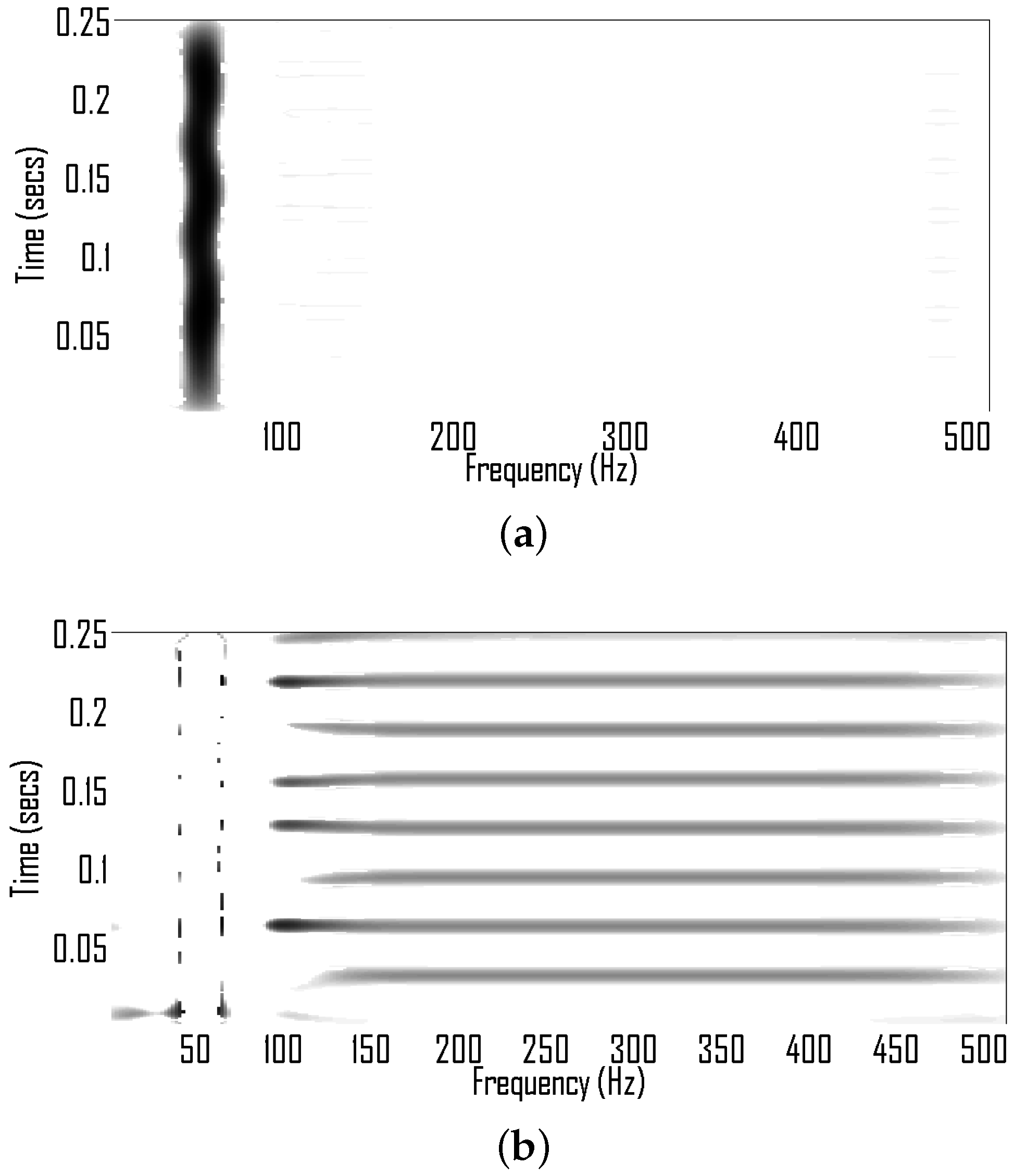
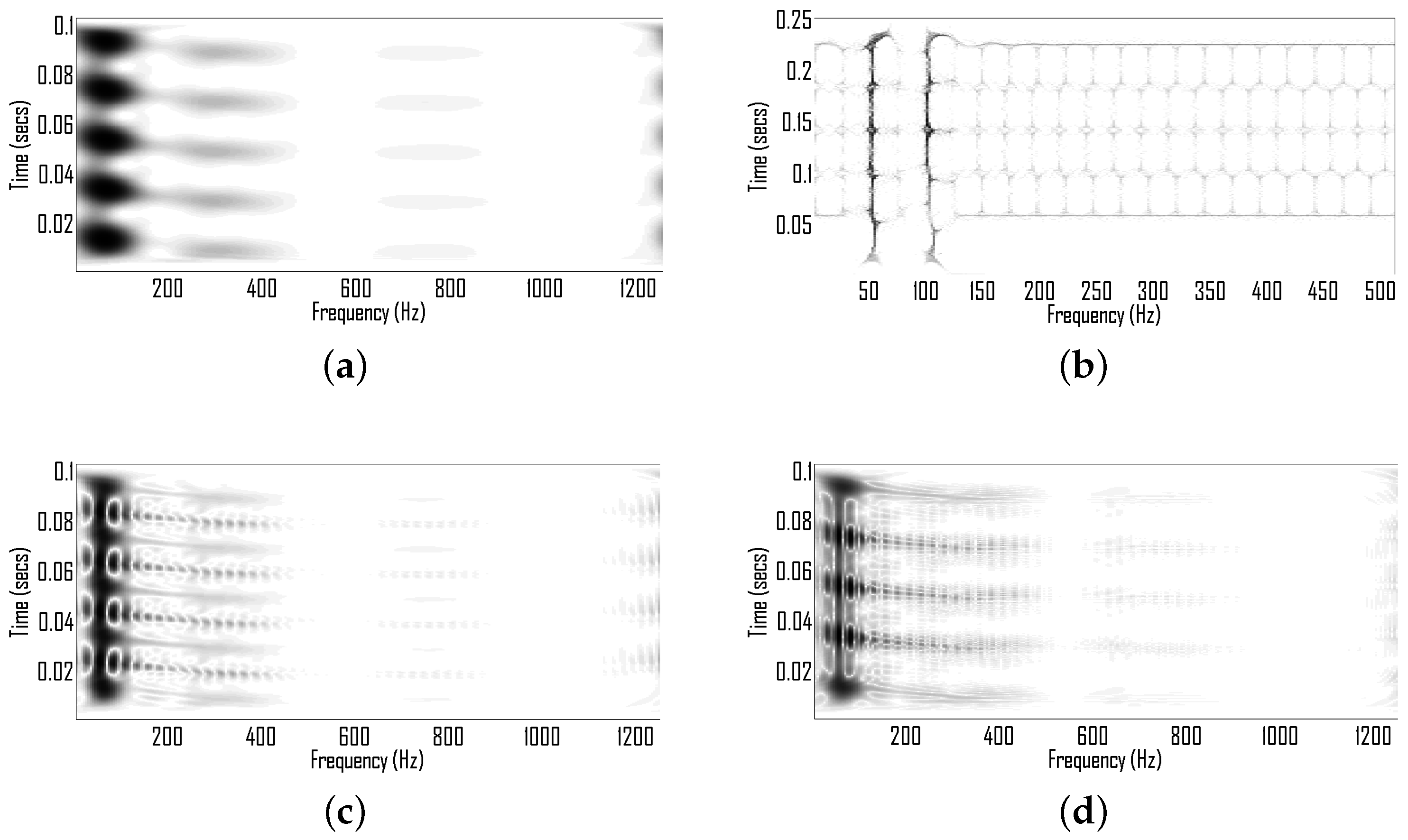
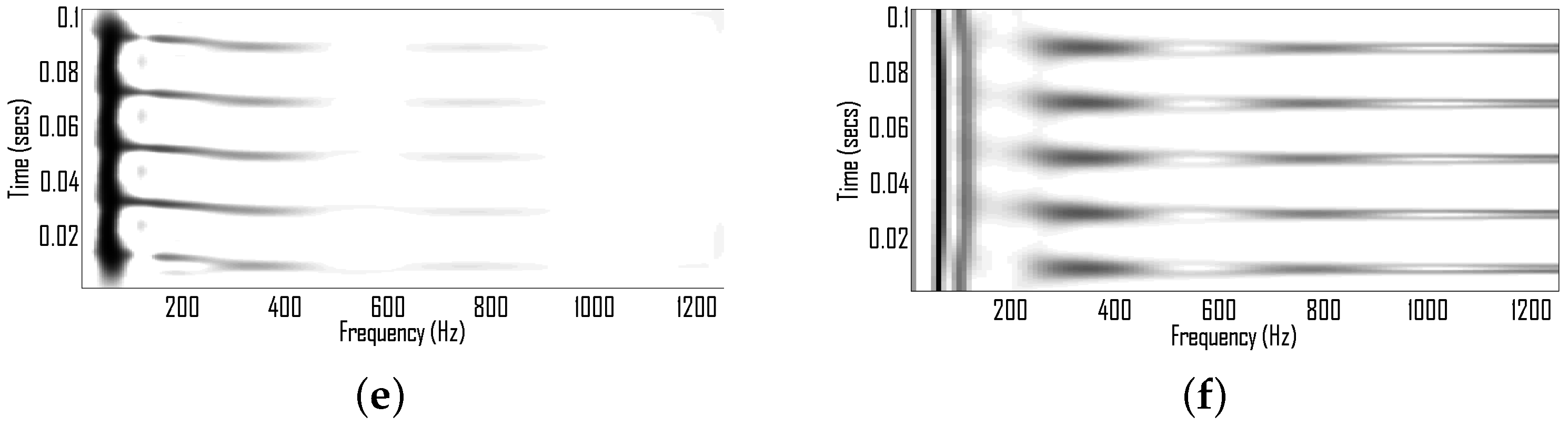
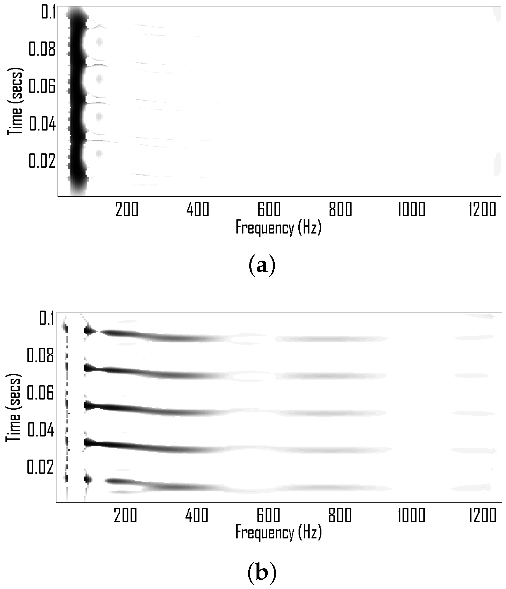
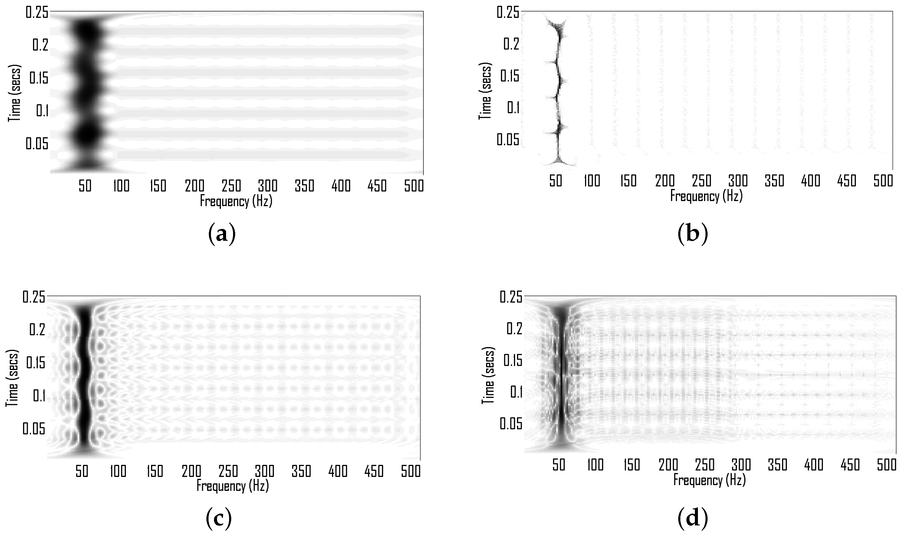
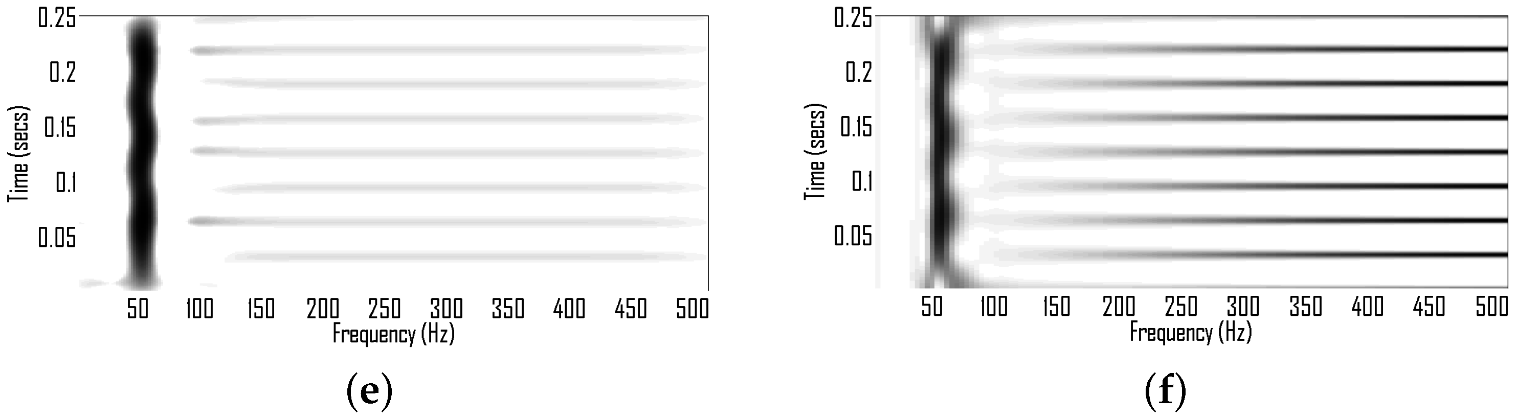
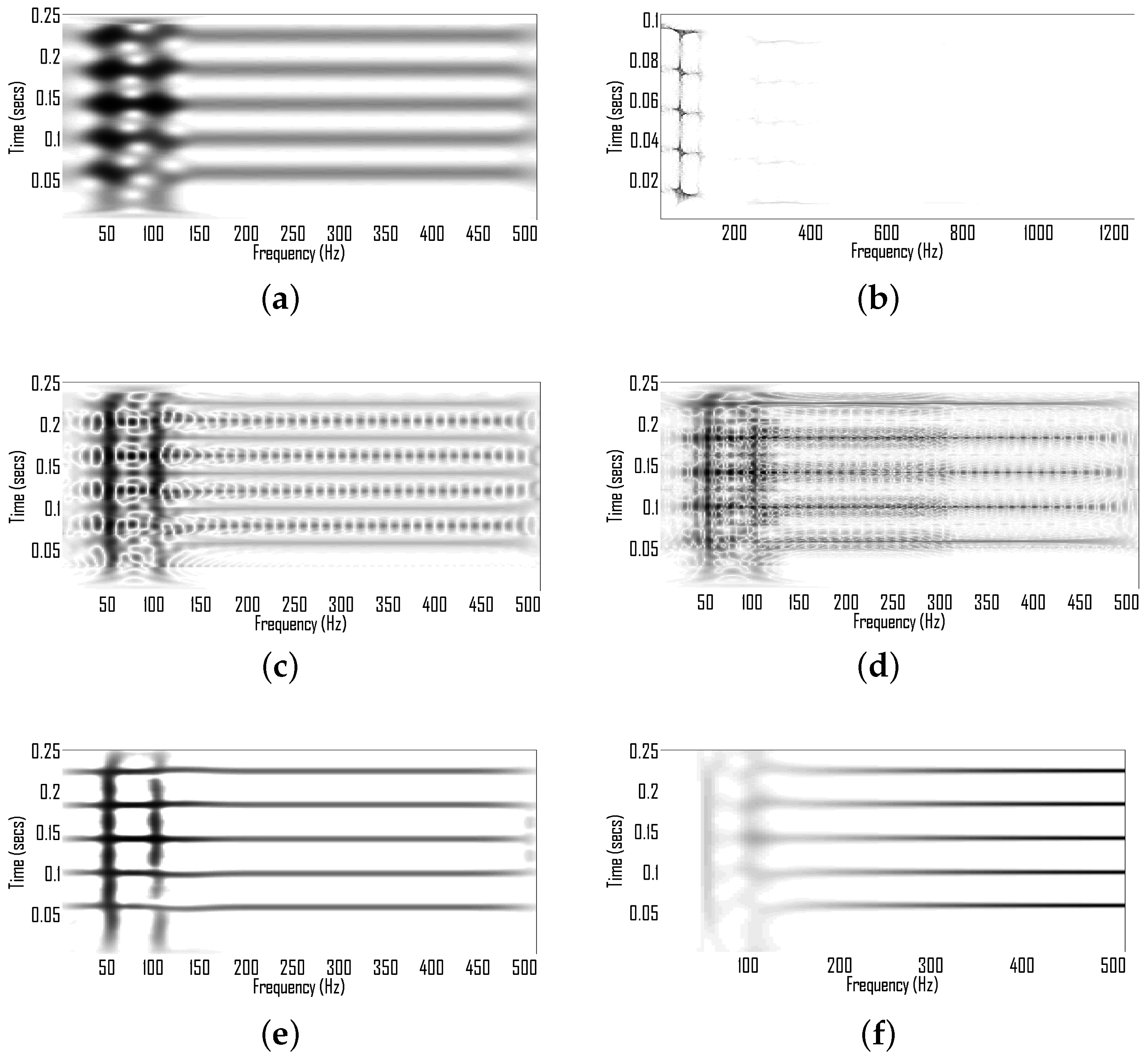
5. Numerical Analysis

To demonstrate the efficacy of the adaptive TFD method in analyzing electrical PQ, extensive simulations for both synthetic and real world electrical power signals are performed.

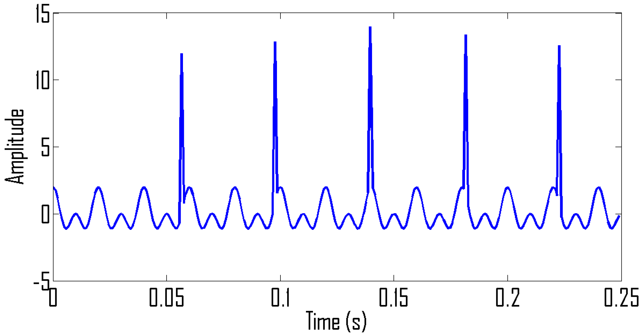
5.1. Synthetic Signals

Let us simulate a scenario when a given signal has both tones and spikes:

$$s(t)=s_{\mathrm{tone}}+s_{\mathrm{spike}},$$

(15)

where the tone part is defined as,

$$s_{\mathrm{tone}}=cos(100\pi t),$$

(16)

and the spike part is given as,

$$s_{\mathrm{spike}}=\sum _{k=0}^N\delta (t-kT),$$

(17)

where $T=1/32s$. The given signal was sampled at 1024 Hz. The time-domain representation of the signal is illustrated in Figure 1.

The signal was analyzed using the state-of-the-art TFDs including the Spectrogram, reassigned Spectrogram [31], modified B distribution (MBD) (a Separable kernel TFD) [12], Gabor Wigner Transform [13] (or marked WVD), S-transform and the proposed adaptive method; the TF plots obtained from all those methods are shown in Figure 2. It is observed that the Spectrogram and reassigned Spectrogram fail to concentrate signal energy for spikes due to their poor energy concentration. The WVD is hard to interpret due to the presence of cross-terms. The MBD suppresses cross-terms to a certain extent, but it is difficult to separate cross-terms from spikes. The Gabor Wigner transform fails to clearly represent spikes due to the overlapping of auto-terms and cross-terms in the WVD.

The S-transform due to its frequency dependent analysis window and the adaptive TFD, due to its locally adaptive smoothing kernel, achieves high concentration of energy for the given signal. Another benefit of the proposed approach is that it can separate TF signatures of spikes and tones using Equations (12) and (13), as indicated in Figure 3.

In order to demonstrate the performance of the proposed method on a more complicated and practical scenario, we consider a signal consisting of f multiple tones in addition to spikes at random and multiple instances. Let us denote such a signal by $s(t)$, which is given by

$$s(t)=s_{\mathrm{tone}}+s_{\mathrm{spike}},$$

(18)

where the tone part is defined as

$$s_{\mathrm{tone}}=cos(100\pi t)+cos(200\pi t),$$

(19)

and the spike part is given as

$$s_{\mathrm{spike}}=\sum _{k=0}^N\delta (t-kT),$$

(20)

where $T=1/24s$. The given signal was sampled at 1024 Hz. The time-domain representation of the signal is illustrated in Figure 4. The signal was analyzed using the same set of TFDs that were used in the earlier example; the TF plots obtained from all those methods are shown in Figure 5. It is observed that the Spectrogram and reassigned Spectrogram fail to concentrate signal energy in the case of spikes. The MBD is hard to interpret due to the presence of cross-terms. The Gabor Wigner transform fails to clearly represent spikes due to overlapping of auto-terms and cross-terms in the WVD. The S-transform achieves high energy concentration for spikes but fails to achieve high energy concentration for tones. The TFD Spectrogram obtained from the proposed method, however, not only resolves close tones but achieves a clear representation of spikes (Figure 5e).

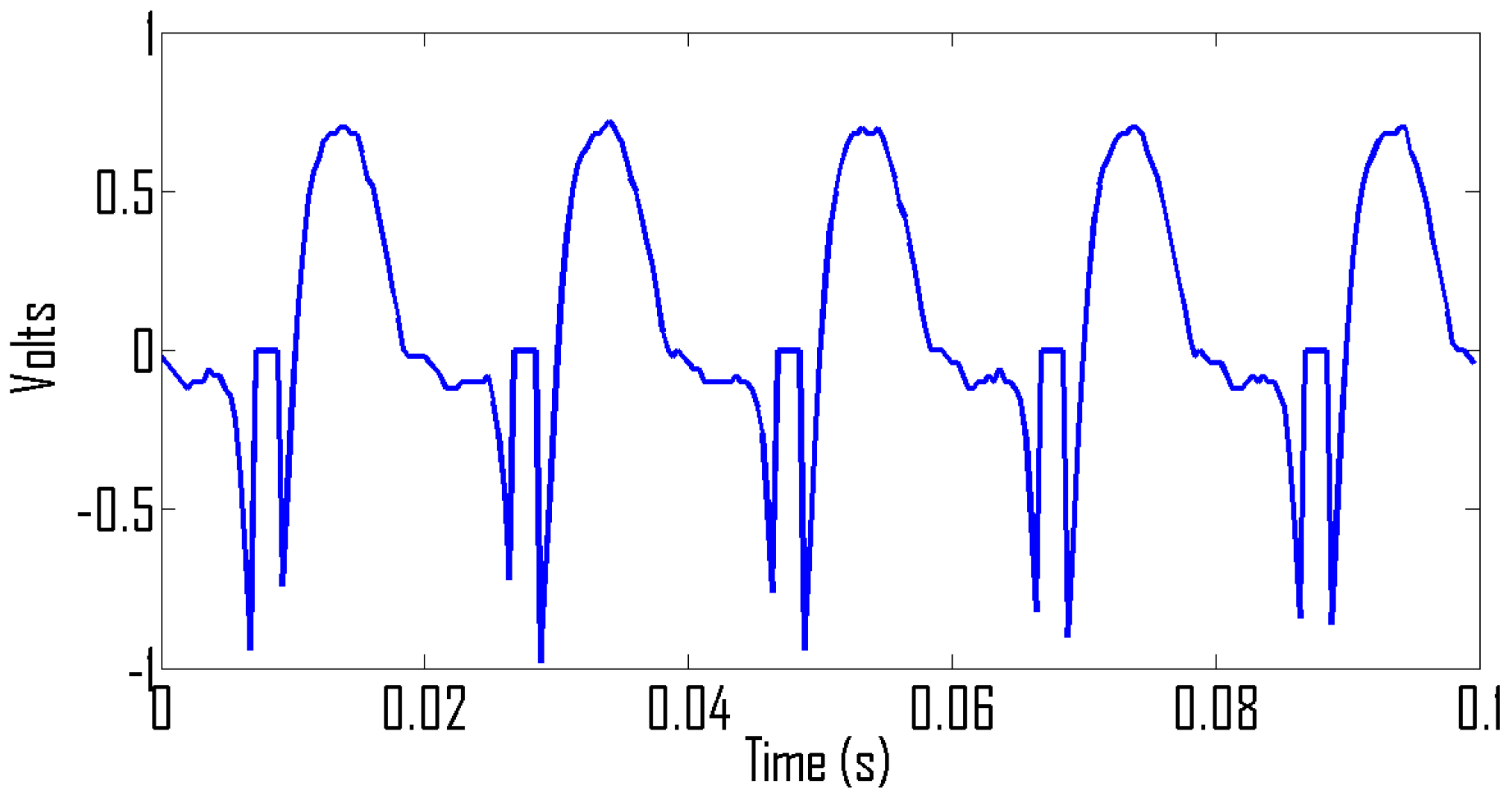
5.2. Real World Signals

Let us now repeat the above experiment for a real world power signal acquired from the soldering iron. The signal is sampled at 2500 Hz and the total duration of signal is $0.1$ s. The time-domain representation of the signal given in Figure 6 indicates that the signal has both sinusoidal and spiky characteristics. The given signal is analyzed from the same set of TFDs that were used in the earlier experiment as shown in Figure 7. The Spectrogram results in a blurred TF representation. The reassigned Spectrogram fail to concentrate energy for spikes. The poor performance of the WVD, MBD and Spectrogram is due to their fixed smoothing kernels that cannot be adapted locally. The Gabor Wigner transform, which is otherwise a useful tool for PQ signals also fails to achieve high energy concentration. The poor performance of the Gabor Wigner transform is due to the overlapping of cross-terms with auto-terms in the WVD. The proposed TFD, due to its local adaptation, achieves high energy concentration for all signal components. Similarly, the S-transform due to frequency dependent window adaptation achieves good energy concentration for both tone and spikes.

Experimental results confirm that the adaptive TFD and S-transform outperform their counterparts in terms of preservation of signal energy for both spikes and tones. However, the adaptive TFD provides additional benefits, i.e., using Equations (12) and (13), we can separately observe TF points belonging to tones and spikes as illustrated in Figure 8. The ratio of spike energy versus tone energy for this experiment is now obtained as: $0.538$. This ratio can also stand as an unanimous quantifier to measure the distribution of energy along spikes for the monitoring of PQ signals.

6. Conclusions

An effective method for the analysis of PQ signals with spiky characteristics has been developed. Extensive computer simulations have been performed to study the performance of the proposed technique in analyzing electrical PQ on both synthetic and real world electrical power signals. The proposed method has been observed to outperform the existing signal analysis techniques including Gabor Wigner transform in terms of its ability to give a clear representation for both spikes and tones. Based on the proposed analysis, it has been concluded that the ratio between the signal energy consumed in spikes and the tone energy is a useful quantifier for the effective monitoring of PQ in electrical power signals. This feature can be integrated with the rest of the features developed as part of other studies for the automatic classification of PQ signals.

References

1. Biswal, B.; Biswal, M.; Mishra, S.; Jalaja, R. Automatic classification of power quality events using balanced neural tree. IEEE Trans. Ind. Electron. 2014, 61, 521–530. [Google Scholar] [CrossRef]
2. Faisal, M.; Mohamed, A.; Shareef, H.; Hussain, A. Power quality diagnosis using time frequency analysis and rule based techniques. Expert Syst. Appl. 2011, 38, 12592–12598. [Google Scholar] [CrossRef]
3. Valtierra-Rodriguez, M.; de Jesus Romero-Troncoso, R.; Osornio-Rios, R.A.; Garcia-Perez, A. Detection and classification of single and combined power quality disturbances using neural networks. IEEE Trans. Ind. Electron. 2014, 61, 2473–2482. [Google Scholar] [CrossRef]
4. Avdakovic, S.; Bosovic, A.; Hasanspahic, N.; Saric, K. Time-frequency analyses of disturbances in power distribution systems. Eng. Rev. 2014, 34, 175–180. [Google Scholar]
5. Khadse, C.B.; Chaudhari, M.A.; Borghate, V.B. Conjugate gradient back-propagation based artificial neural network for real time power quality assessment. Int. J. Electr. Power Energy Syst. 2016, 82, 197–206. [Google Scholar] [CrossRef]
6. Hajian, M.; Foroud, A.A.; Abdoos, A.A. New automated power quality recognition system for online/offline monitoring. Neurocomputing 2014, 128, 389–406. [Google Scholar] [CrossRef]
7. Hajian, M.; Foroud, A.A. A new hybrid pattern recognition scheme for automatic discrimination of power quality disturbances. Measurement 2014, 51, 265–280. [Google Scholar] [CrossRef]
8. Szmajda, M.; Górecki, K.; Mroczka, J. Gabor transform, spwvd, gabor-wigner transform and wavelet transform-tools for power quality monitoring. Metrol. Meas. Syst. 2010, 17, 383–396. [Google Scholar] [CrossRef]
9. Huang, N.; Lu, G.; Cai, G.; Xu, D.; Xu, J.; Li, F.; Zhang, L. Feature Selection of Power Quality Disturbance Signals with an Entropy-Importance-Based Random Forest. Entropy 2016, 18, 44. [Google Scholar] [CrossRef]
10. Hlawatsch, F.; Boudreaux-Bartels, G.F. Linear and quadratic time-frequency signal representations. IEEE Signal Process. Mag. 1992, 9, 21–67. [Google Scholar] [CrossRef]
11. Hlawatsch, F. Interference terms in the Wigner distribution. Digit. Signal Process. 1984, 84, 363–367. [Google Scholar]
12. Boashash, B.; Khan, N.A.; Ben-Jabeur, T. Time–frequency features for pattern recognition using high-resolution TFDs: A tutorial review. Digit. Signal Process. 2015, 40, 1–30. [Google Scholar] [CrossRef]
13. Pei, S.C.; Ding, J.J. Relations between Gabor transforms and fractional Fourier transforms and their applications for signal processing. IEEE Trans. Signal Process. 2007, 55, 4839–4850. [Google Scholar] [CrossRef]
14. Kalyuzhny, A.; Zissu, S.; Shein, D. Analytical study of voltage magnification transients due to capacitor switching. IEEE Trans. Power Deliv. 2009, 24, 797–805. [Google Scholar] [CrossRef]
15. Sumner, M.; Abusorrah, A.; Thomas, D.; Zanchetta, P. Real Time Parameter Estimation for Power Quality Control and Intelligent Protection of Grid-Connected Power Electronic Converters. IEEE Trans. Smart Grid 2014, 5, 1602–1607. [Google Scholar] [CrossRef]
16. Memon, A.P.; Uqaili, M.A.; Memon, Z.A.; Adil, W.; Keerio, M.U. Classification Analysis of Power System Transient Disturbances with Software Concepts. Sci. Int. 2014, 26, 1447–1456. [Google Scholar]
17. He, S.; Li, K.; Zhang, M. A New Transient Power Quality Disturbances Detection Using Strong Trace Filter. IEEE Trans. Instrum. Meas. 2014, 63, 2863–2871. [Google Scholar] [CrossRef]
18. Liu, Z.; Cui, Y.; Li, W. Combined power quality disturbances recognition using wavelet packet entropies and S-transform. Entropy 2015, 17, 5811–5828. [Google Scholar] [CrossRef]
19. Dash, P.; Panigrahi, B.; Panda, G. Power quality analysis using S-transform. IEEE Trans. Power Deliv. 2003, 18, 406–411. [Google Scholar] [CrossRef]
20. Lee, I.W.; Dash, P.K. S-transform-based intelligent system for classification of power quality disturbance signals. IEEE Trans. Ind. Electron. 2003, 50, 800–805. [Google Scholar] [CrossRef]
21. Laila, D.S.; Messina, A.R.; Pal, B.C. A refined Hilbert–Huang transform with applications to interarea oscillation monitoring. IEEE Trans. Power Syst. 2009, 24, 610–620. [Google Scholar] [CrossRef] [Green Version]
22. Huang, N.E.; Shen, Z.; Long, S.R.; Wu, M.C.; Shih, H.H.; Zheng, Q.; Yen, N.C.; Tung, C.C.; Liu, H.H. The Empirical Mode Decomposition and the Hilbert Spectrum for Nonlinear and Non-Stationary Time Series Analysis. R. Soc. 1998, 454, 903–995. [Google Scholar] [CrossRef]
23. Mohammadi, M.; Pouyan, A.A.; Khan, N.A. A highly adaptive directional time–frequency distribution. Signal Image Video Process. 2016, 10, 1369–1376. [Google Scholar] [CrossRef]
24. Khan, N.A.; Boashash, B. Multi-component instantaneous frequency estimation using locally adaptive directional time frequency distributions. Int. J. Adapt. Control Signal Process. 2016, 30, 429–442. [Google Scholar] [CrossRef]
25. Khan, N.A.; Ali, S.; Jansson, M. Direction of arrival estimation using adaptive directional time-frequency distributions. Multidimens. Syst. Signal Process. 2016, in press. [Google Scholar]
26. Khan, N.A.; Ali, S. Classification of EEG Signals Using Adaptive Time-Frequency Distributions. Metrol. Meas. Syst. 2016, 23, 251–260. [Google Scholar] [CrossRef]
27. Cho, S.H.; Jang, G.; Kwon, S.H. Time-frequency analysis of power-quality disturbances via the Gabor–Wigner transform. IEEE Trans. Power Deliv. 2010, 25, 494–499. [Google Scholar]
28. Khan, N.A.; Jaffri, M.N.; Shah, S.I. Modified Gabor Wigner transform for crisp time frequency representation. In Proceedings of the IEEE International Conference on Signal Acquisition and Processing, Kuala Lumpur, Malaysia, 3–5 April 2009; pp. 119–122.
29. Ajab, M.; Taj, I.A.; Khan, N.A. Comparative analysis of variants of Gabor-Wigner transform for cross-term reduction. Metrol. Meas. Syst. 2012, 19, 499–508. [Google Scholar]
30. Bastiaans, M.J.; Alieva, T.; Stankovic, L. On rotated time-frequency kernels. IEEE Signal Process. Lett. 2002, 9, 378–381. [Google Scholar] [CrossRef]
31. Auger, F.; Flandrin, P. Improving the readability of time-frequency and time-scale representations by the reassignment method. IEEE Trans. Signal Process. 1995, 43, 1068–1089. [Google Scholar] [CrossRef]
Figure 1. A synthetic power quality signal having both tones and spikes.
Energies 09 00933 g001
Figure 2. TF plots of the synthetic signal, given by Equation (15), (a) Spectrogram (hamming window of length 45); (b) reassigned Spectrogram; (c) MBD ( β = 0 . 1 and lag window of length 64); (d) Gabor Wigner transform (Gabor transform of window length 45 is used); (e) the adaptive TFD ( a = 3 and b = 8 ); and (f) the S-transform.
Energies 09 00933 g002aEnergies 09 00933 g002b
Figure 3. Separation of TF representations of tone and spike using direction of signal energy (a) TF representation of tone; and (b) TF representation of spikes.
Energies 09 00933 g003
Figure 4. A synthetic PQ signal composed of two tones and spikes.
Energies 09 00933 g004
Figure 5. Time-frequency plots of the synthetic signal, given by (18), (a) Spectrogram (hamming window of length 45); (b) reassigned Spectrogram; (c) MBD ( β = 0 . 1 and lag window of length 64); (d) Gabor Wigner transform (Gabor transform of window length 45 is used); (e) the adaptive TFD ( a = 3 and b = 8 ); and (f) the S-transform.
Energies 09 00933 g005
Figure 6. A real world PQ signal showing both tones and spikes.
Energies 09 00933 g006
Figure 7. TF plots of a real world signal acquired from iron having spikes. (a) Spectrogram (hamming window of length 45); (b) reassigned Spectrogram; (c) MBD ( β = 0 . 1 and lag window of length 64); (d) Gabor Wigner transform (Gabor transform of window length 45 is used); (e) the adaptive TFD ( a = 3 and b = 8 ); and (f) the S-transform.
Energies 09 00933 g007aEnergies 09 00933 g007b
Figure 8. Separation of TF representation of tones and spikes using the direction of signal energy (a) TF representation of tones; and (b) TF representation of spikes.
Energies 09 00933 g008