Article

Using Trajectory Clusters to Define the Most Relevant Features for Transient Stability Prediction Based on Machine Learning Method

School of Electrical Engineering, Beijing Jiaotong University, Beijing 100044, China
*
Author to whom correspondence should be addressed.
Energies 2016, 9(11), 898; https://doi.org/10.3390/en9110898
Submission received: 28 July 2016 / Revised: 25 October 2016 / Accepted: 25 October 2016 / Published: 1 November 2016
(This article belongs to the Special Issue Electric Power Systems Research 2017)

Abstract

:
To achieve rapid real-time transient stability prediction, a power system transient stability prediction method based on the extraction of the post-fault trajectory cluster features of generators is proposed. This approach is conducted using data-mining techniques and support vector machine (SVM) models. First, the post-fault rotor angles and generator terminal voltage magnitudes are considered as the input vectors. Second, we construct a high-confidence dataset by extracting the 27 trajectory cluster features obtained from the chosen databases. Then, by applying a filter–wrapper algorithm for feature selection, we obtain the final feature set composed of the eight most relevant features for transient stability prediction, called the global trajectory clusters feature subset (GTCFS), which are validated by receiver operating characteristic (ROC) analysis. Comprehensive simulations are conducted on a New England 39-bus system under various operating conditions, load levels and topologies, and the transient stability predicting capability of the SVM model based on the GTCFS is extensively tested. The experimental results show that the selected GTCFS features improve the prediction accuracy with high computational efficiency. The proposed method has distinct advantages for transient stability prediction when faced with incomplete Wide Area Measurement System (WAMS) information, unknown operating conditions and unknown topologies and significantly improves the robustness of the transient stability prediction system.

1. Introduction

With the expansion of the scale of the power grid and the implementation of mixed transmission, the dynamic characteristics of the power system have become more complex. Meanwhile, these factors highlight the importance of power system stability analysis and control. The transient stability analysis methods can generally be divided into time-domain simulation methods, straightforward methods based on the transient energy function [1], extended equal area methods [2] and data-mining methods [3,4,5,6,7,8,9,10,11,12,13,14,15,16]. However, the traditional methods, like the time-domain simulation and transient energy function methods, have some disadvantages, such as requiring accurate parameters and information about the network configuration during the fault and being time consuming.
In recent years, researchers have paid increasing attention to machine learning techniques for fast online transient stability assessment. The rapid spread of Wide Area Measurement System (WAMS) deployments has made machine learning-based methods more applicable. Using offline learning on the measured dynamic responses or simulation database, useful information can be extracted to represent the relationship between post-fault variation and the system stability status. Thus, online stability prediction can be achieved. For instance, artificial neural networks (ANNs) have been proposed as a promising approach to solve complex power system protection and control problems instead of simulating the power system equations for transient stability assessment (TSA). These approaches can quickly obtain a nonlinear mapping of the relationship between the input and the output data and can obtain approximate solutions of power system’s differential equations [4]. There are two ways to use ANNs for power system TSA: as a regression function to predict the transient stability degree [5,6], such as the critical clearing time and system stability margin, and as a classifier to directly classify the system into either stable or unstable states [15]. There are many different types of neural networks, such as Multilayer Perceptron Neural Network (MLP NN) and radial basis function (RBF) NN, which can be used in different applications.
In [7], the application of decision tree (DT) theory based on the R-Rdot strategy was proposed for loss of synchronism detection. The same technique has been used in [8] for wide-area response-based control using synchronized phasor measurements.
Compared with other methods, such as neural networks, support vector machine (SVM) has multiple merits. It can handle problems of high dimensionality in restricted training samples, and it has promising computational capabilities. Further, it has great generalization ability. Reference [17] proposed an SVM classifier and a set of pre-identified voltage variation trajectory templates to predict the transient stability status. The measured bus voltages were compared with the templates to evaluate a fuzzy membership that indicated the similarity between the measured voltage variations and the templates. The similarity values were input into the trained SVM to make the classification.
Reference [18] proposed an SVM classifier that differed from [17]. The classifier directly used sampled values of the measured voltage magnitudes at the generator buses. Thus, it is simpler and slightly faster than the method proposed in [17,19]. Furthermore, the paper investigated the effectiveness of alternative inputs, namely, the center of inertia rotor angle and rotor speed measurements, to predict the stability.
Transient stability can be considered rotor angle stability; the post-fault generator terminal voltage variation has no direct correlation with rotor angle stability. However, the methods proposed in [18,19,20,21] are based on the terminal voltage amplitude as the input. The selection of the terminal voltage as the input for prediction has not been thoroughly discussed. Moreover, if the original data of the WAMS system are incomplete, such as due to communication errors or parts of the signal channel being jammed, these methods may fail. Reference [22] studied data mining for the characteristics of fuzzy multidimensional time series data and noted that in multidimensional time series data, the relationship between data collection and the overall characteristics reflect the key information of the data sets. Therefore, the extraction and selection of the wide-area fault features that are closely related to the system transient stability are of great importance.
In this paper, a novel method is presented to build a transient stability classifier based on a new feature extraction and selection approach. This approach utilizes geometric measures of the post-fault trajectory clusters of rotor angles and generator terminal voltages to define 27 global cluster features to improve the prediction performance of the constructed classifiers. In the first stage, our proposed method is based on the selection of the most relevant extracted features via the filter–wrapper technique. The RELIEF algorithm [23] is used as a filter. The details of the RELIEF algorithm are elaborated in Section 2.3. The construction of the classifiers is based on SVMs. Additionally, this classifier can return a confidence score for each prediction by modifying the SVM implementation. Then, we use the area under the ROC curve (AUC) [24] to evaluate the SVM models to determine the optimal feature subset that represents the most relevant features of the TSA problem. We call this optimal feature subset the global trajectory clusters feature subset (GTCFS). Then, the stability prediction models are constructed based on the obtained GTCFS. In the second stage, comprehensive simulations are conducted on a New England 39-bus system under various operating conditions, load levels and topologies, and the transient stability predicting performance is tested. The proposed stability classifiers based on SVM and GTCFS are verified to possess excellent prediction accuracy with high computational efficiency, strong generalization ability to unknown load levels and topologies, independent of the system scale, and great robustness to incomplete WAMS information.
This paper is arranged as follows: the introduction is given in Section 1. The details of the proposed methodology are presented in Section 2. Then, simulations and a discussion of the performance of the proposed method are provided in Section 3. Finally, Section 4 summarizes the concluding remarks.

2. Methodology

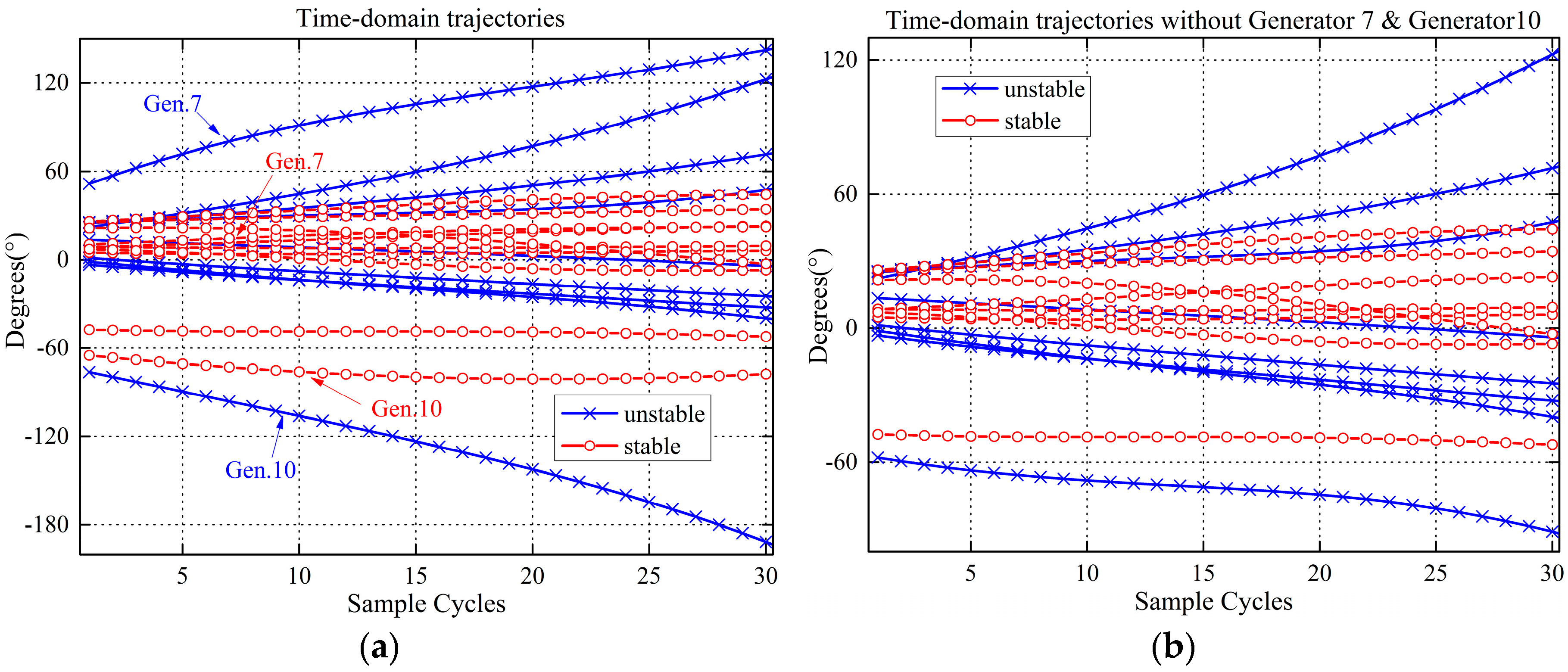
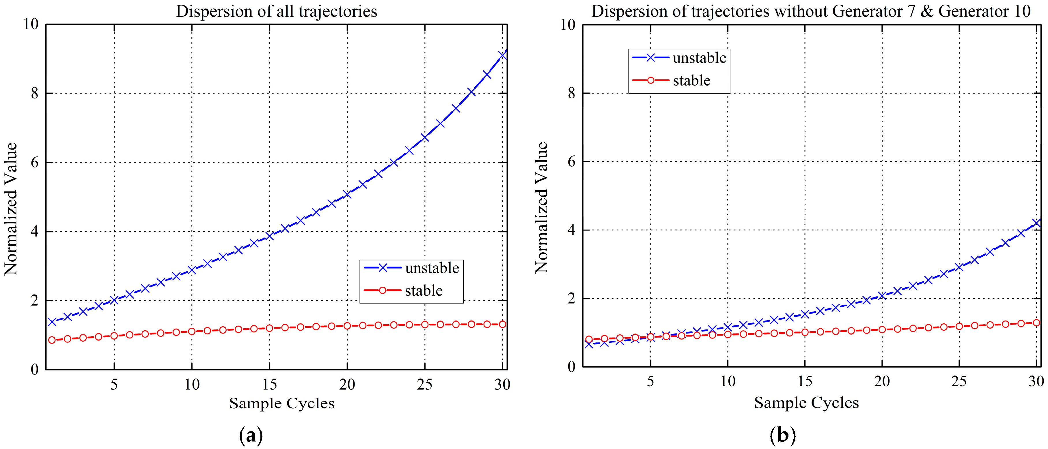
2.1. Observations on Post-Fault Trajectories

In machine learning, the attributes are required to fully reveal the characteristic differences among input samples. However, the most confusing characteristic is the subjectivity of the attribute extraction. In previous studies, several electrical variables, such as post-fault variations of rotor angles, rotor speeds, and voltage magnitudes, have been used as the indicators of stability. The inputs to the intelligent classifier were directly sampled values of these variables. Reference [18] selected all the perturbed generator voltage amplitudes as the initial inputs, so the number of inputs increased exponentially with the number of generators, which caused difficulties with online applications. However, in practical application, regardless of the type of electrical variables used as the input, if the measurements of some generators are missing, the input data channel is incomplete, and the mapping output may have large deviation from the actual result.
Taking the New England 39-bus system for example, several transient stability simulations have been performed. One stable case and another unstable case were obtained. The selected cases are two special cases that are close to the critical stability boundary. The time-domain variation of the generator rotor angles is shown in Figure 1a. One sampling value was recorded at each cycle by a PMU device, and the rotor angle trajectories of the first thirty sampling cycles after the fault cleared were observed. In the actual situation, some PMU information may be missing due to communication failure. When the trajectories of Generator 7 and Generator 10 are missing, the corresponding variations are shown in Figure 1b, which shows that if these two trajectories are missing, the stable and unstable trajectories are nearly mixed, especially for the first 15 cycles. Therefore, if these trajectories are selected as the input to construct the classifier, it would be difficult to correctly determine whether they are stable.
If we examine some of the overall features of the whole trajectory clusters (as defined in Section 2.2), for example, the dispersion degree of these 10 trajectories, interesting results may be obtained. The dispersion variation of the 10 trajectories and the 8 trajectories without Generator 7 and Generator 10 are shown in Figure 2a,b.
Figure 2 shows that even when these two trajectories are missing, the dispersion of the two categories can be distinguished. Moreover, if we only use the first 15 cycles of sampling data, it is not misclassified. Therefore, by comparison of Figure 1 and Figure 2, we can assume that the overall features of the whole trajectory clusters have outstanding advantages over the time-domain trajectory vectors themselves for the transient stability prediction problem. The merits are based on three factors: (1) The overall features of the trajectory clusters have more comprehensive and global information than single trajectory vectors; (2) the overall features used as the input of the classifier have better computational efficiency, independent of the system scale; and (3) if part of the information is missing, the overall features are still effective for stability classification; however, the classifier based on the trajectories themselves may lead to incorrect classification results.

2.2. Trajectory Clusters Feature Extraction

Through observations of a large number of rotor angle and voltage magnitude trajectory curves, some overall features could be constructed to find the global and essential characteristics of both the rotor angle and the voltage magnitude trajectories. In this paper, several new features are defined based on the geometric attributes of trajectory clusters, which are shown as follows:
1. Basic cluster features
Trajectory clusters can be represented by { x i j } m × n , where m represents the number of generator terminal voltage magnitudes or rotor angle trajectories, and n is the number of samples. The arithmetic mean of the trajectory cluster can be defined as:
c j = 1 m i = 1 m x i j
The degree of dispersion is defined as the mean of the squared Euclidean distance to the mean:
d j = 1 m [ i = 1 m | x i j c j | 2 ]
The upper and lower envelopes are defined as:
{ max ( x j ) } , j = 1 , 2 , ... , n , { min ( x j ) } , j = 1 , 2 , ... , n
The mid-range is defined as:
m c j = 1 2 ( max ( x j ) min ( x j ) ) , j = 1 , 2 , ... , n
2. Gradient and curvature features
The gradient of the trajectory clusters is the first-order derivative of the basic features and can be defined as:
r j = 1 h | x j + 1 x j | , j = 1 , 2 , ... , n 1
where h is the time sampling interval, which can be set to 1 to simplify the calculation.
The curvature of the trajectory can be defined as:
C j = 1 h 2 [ i = 1 m ( x i , j 1 2 x i , j + x i , j + 1 ) 2 ] 1 / 2 , j = 2 , ... , n 1
Similarly, the gradient or curvature of the arithmetic mean, degree of dispersion and envelope can also be defined. When the curvature of dispersion or the envelope is calculated, Equation (6) can still hold when m = 1, and m no longer represents the generator number but the number of trajectories.
3. Acceleration features
The acceleration features are the second-order derivatives of the basic features. The acceleration of the trajectory clusters can be defined as:
a c j = 1 h [ r c j + 1 r c j ] , j = 1 , 2 , ... , n 2
where r c is the gradient of the trajectory clusters.
There are 27 cluster features defined in this paper. The feature definitions are given in Table 1.
As shown above, we provided a sufficient number of features for the prediction problem. Nevertheless, some features may be redundant for a certain dataset. In practice, the number of features be as small as possible. Thus, in a previous stage of the process, a feature selection method is applied to select the minimum optimal set of characteristics. The specific approaches are presented below.

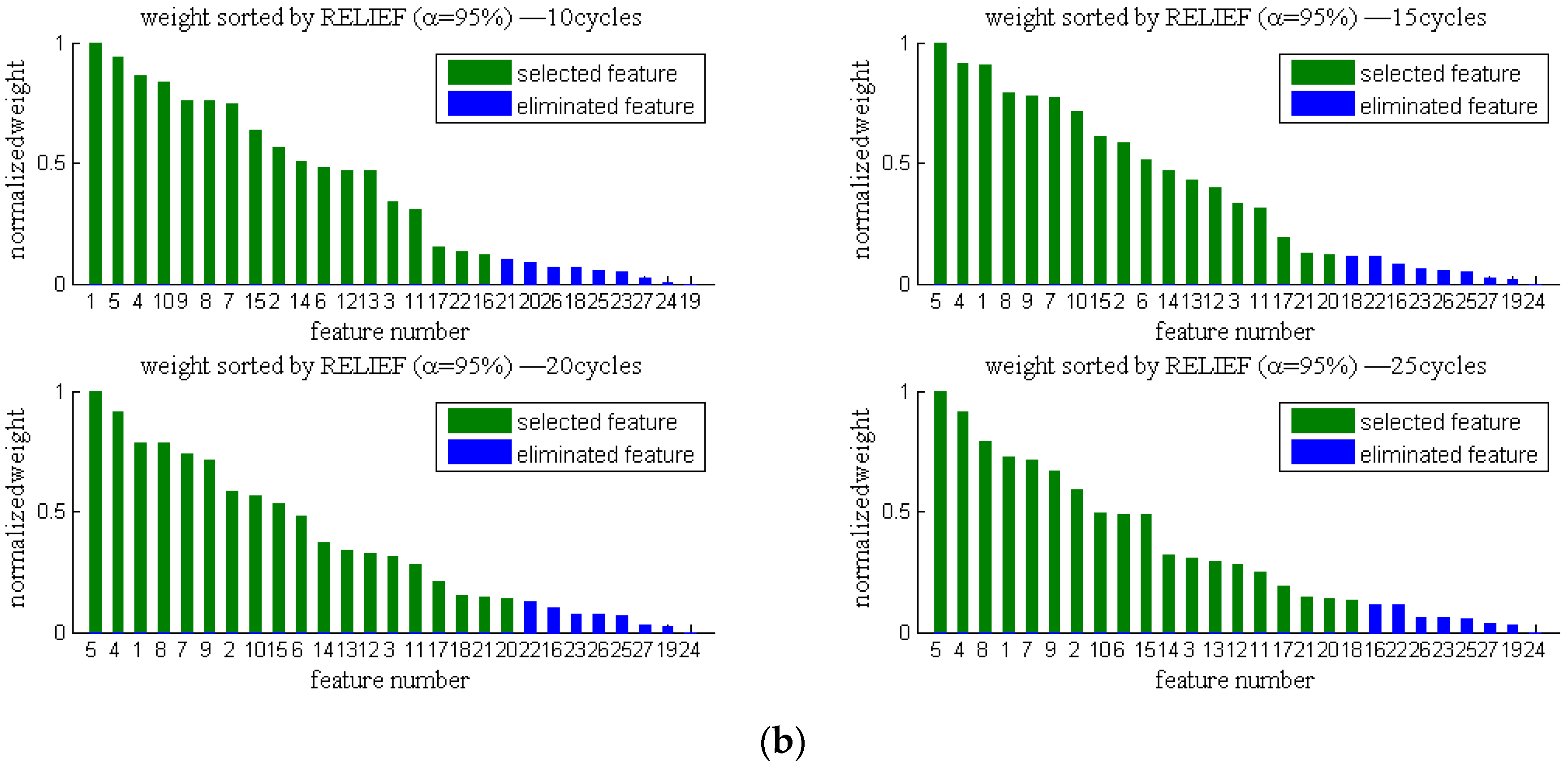
2.3. Feature Selection: RELIEF Algorithm

In machine learning theory, filtering out irrelevant or redundant features can greatly improve the learning performance of classifiers. This reduction in the number of features, also known as feature selection, allows for better training efficiency by reducing the search space for most of the parameters of the model [25,26]. The smaller the number of features, the easier the final prediction model is to process and interpret. In our specific case, we are interested in studying which of the 27 initial features are the most relevant to predicting the transient stability status. Two general approaches are commonly applied in the machine learning literature for feature selection: filter selection methods and wrapper selection methods. In the filtering approach, feature selection is performed as a preprocessing step prior to the learning algorithm. This preprocessing step measures the general characteristics of the training set to select the most important features and to discard those that are irrelevant. In contrast, wrapper methods use the machine learning classification model itself to extract the relevant features. This entails a much greater computational cost since for every subset of features selected by the method, the whole classifier has to be optimized and evaluated again. In this study, the following hybrid method is proposed, combining the advantages of both approaches.
A filter feature selection algorithm called RELIEF [23] was applied, which proved to be very simple and efficient for evaluating feature qualities. The key idea of the RELIEF algorithm is to estimate the quality of features that have weights greater than the thresholds using the difference in the feature value between a given instance and the two nearest instances (called HIT and MISS). In the RELIEF algorithm, the first step is to randomly select an instance and find the nearest instance that belongs to the same class (nearest HIT) and the nearest instance that belongs to a different class (nearest MISS). The second step is to calculate the differences in features between instances and update the weights. The features with weights greater than the threshold are selected as relevant features. The pseudo-code of the RELIEF algorithm is shown in Algorithm 1.
We assume that examples R 1 , R 2 , , R m (line 3) in the instance space are described by a vector of attributes A i , i = 1 , 2 , , a (line 5), where a is the number of explanatory attributes labelled with the target value τ j , j = 1 , 2 , , m . The examples are therefore points in the a -dimensional space. R i (line 3) represents the cluster features calculated based on Table 1 but not the original variables. For that purpose, given a randomly selected instance R i (line 3), RELIEF searches for its two nearest neighbors: one from the same class, called the nearest hit H, and the other from a different class, called the nearest miss M (line 4). The distance between two instances is calculated based on the Euclidean distance. The quality estimation W[A] is updated for all features A depending on their values of R i , M, and H (line 5 and 6). If instances R i and H have different values of feature A, then feature A separates two instances with the same class, which is not desirable, so we decrease the quality estimation W[A]. In contrast, if instances R i and M have different values of feature A, then feature A separates two instances with different class values, which is desirable, so we increase the quality estimation W[A]. Function diff ( A , I 1 , I 2 ) (line 6) calculates the difference between the values of attribute A for two instances, I 1 and I 2 . For numerical attributes, it was originally defined as:
diff ( A , I 1 , I 2 ) = | v a l u e ( A , I 1 ) v a l u e ( A , I 2 ) | max ( A ) min ( A )
Algorithm 1. Pseudo-code of the RELIEF algorithm.
Input: for each training instance, a vector of attribute values and the class value
Output: the vector W of estimations of the qualities of attributes
1. set all weights W[A] = 0;
2. for i = 1 to m do begin
3.  randomly select an instance R i ;
4.  find nearest hit H and nearest miss M;
5.  for A = 1 to a do
6.   W [ A ] = W [ A ] - diff ( A , R i , H ) / m + diff ( A , R i , M ) / m ;
7.  end;
8. end;
9. The selected feature set is { i | W > τ } , where τ is a threshold.

2.4. SVM Classifier

SVM is a classification and regression paradigm that was developed by Vladimir Vapnik [27,28]. The SVM approach is popular in the literature related to classification and regression problems because of its good generalization capability and its superiority over other machine learning paradigms. SVMs were originally designed for binary-class classification; hence, it is straightforward to use this paradigm for the prediction of the power system transient stability status.
Consider a training data set of N points ( x i , y i ) , i = 1 , ... , N , where x i R n is an n-dimensional input vector and y i R is the associated output value of x i . The aim of SVMs is to construct a separating hyperplane as the decision surface that divides the set of examples such that all points with the same label are on the same side of the hyperplane. Meanwhile, the margin of decision boundaries is optimized.
SVM expresses the classification output in terms of a linear combination of examples in the training data, in which only a fraction of the data points, called support vectors, have nonzero coefficients. The support vectors capture the critical information to construct the hyperplane using the training set. In its basic form, an SVM classifies a pattern vector X into classes based on the support vectors x i and their corresponding classes y i as:
y = s i g n { i = 1 M α i y i K ( x i , x ) + b }
where M is the number of support vectors; K ( · , · ) is a symmetric positive-definite kernel function that can be freely chosen and subject to fairly mild constraints, i.e., the Mercer conditions. The parameters α i and b are determined by a linearly constrained quadratic programming (QP) problem, which can be efficiently implemented through a sequence of smaller scale, sub-problem optimizations or an incremental scheme that adjusts the solution one training point at a time. Most of the training data x i has zero coefficients. The nonzero coefficients returned by the constrained QP optimization define the support vector set. In general, for mass nonlinear and inseparable data, α i and offset b of the Lagrange multipliers are calculated by solving quadratic Equation (10) with constraints (11):
min i = 1 N α i 1 2 i , j = 1 N α i α j y i y j K ( x i , x j )
s . t . i = 1 N α i y i = 0 0 α i C , i = 1 , , N
The SVM prediction model is built on the structural risk minimization principle, which equips the model with greater generalization ability. SVM can map complex nonlinear relationships between the input and output. Additionally, the learning process focuses on those operation points near the decision boundary. Therefore, it is suitable for TSA. Furthermore, the kernel computation of SVM only involves inner products of the data vectors in the feature space. Thus, fast training results are obtained even with a large number of input features. The SVM classifier was implemented using the LIBSVM toolbox [29] in MATLAB.
The most common SVM kernel in the literature is the Gaussian or RBF kernel [27], which is defined by:
K ( x , x i ) = exp ( γ x x i 2 ) , γ > 0
where parameter γ > 0 controls the region of influence of every support vector.
The SVM training requires optimization of α i and b of the hyperparameters of the model, which are typically estimated by grid-search and cross-validation [30]. For the RBF kernel, hyperparameters C and γ must be optimized. The training process comprises a grid-search to find the best values of parameters C and γ . The grid-search procedure is time consuming, whereas the training of an SVM with modified parameters ( C and γ ) is fast. For example, when 10-cycle samples of generator rotor angles were recorded, using a MATLAB toolbox implemented on a PC with Intel Core 2 2.6-GHz processor and 4 GB of RAM, the training process took approximately 3.5 s. Therefore, in practice, if parallel computing is used to obtain the optimized parameters, the computational costs can be minimized.
We also utilize a confidence score to measure the confidence of the prediction results. The confidence score is the absolute difference in the probabilities returned by SVM for each sample. For this binary classification problem of transient stability prediction, two probability values that represent the chance to be a member of the two categories are provided after the SVM training process. A sample is classified as positive or negative according to its highest probability. The details of how to obtain the probabilities of the multi-class classification can be found in Wu et al. [31]. In this binary classification problem, given observation x and class label y , we assume that the estimated class probabilities μ i j = P ( y = i | y = i o r j , x ) are available. The class probabilities are estimated by r i j :
r i j = P ( y = i | y = i o r j , x ) 1 1 + e A f + B
where A and B are estimated by minimizing the negative log-likelihood function using known training data, and f is the decision values of these training data. In Zhang et al. [32], the fact that the SVM decision can be easily clustered at ±1, making the estimated probability in (13) an inaccurate classification, is recalled. Therefore, five-fold cross-validation to obtain the decision values is conducted for the experimental results. The next step is to obtain p i from these r i j by solving the following optimization problem presented in Wu et al. [31].

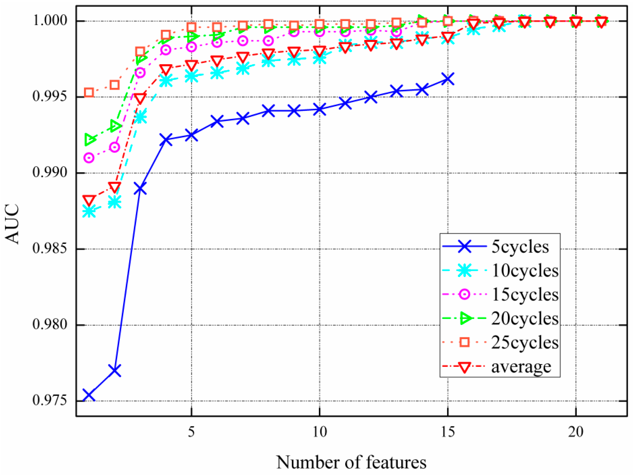
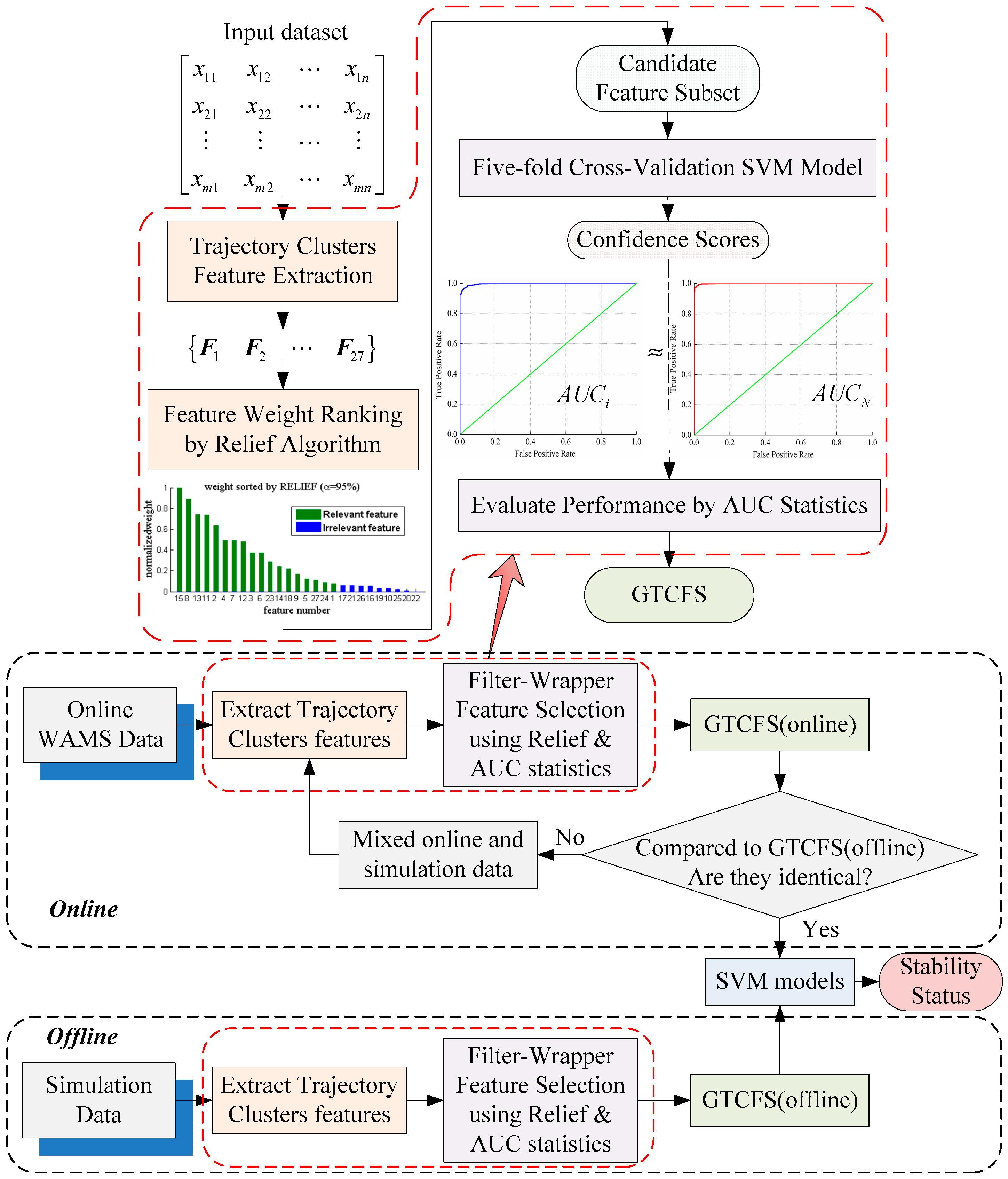
2.5. AUC Based Global Trajectory Clusters Feature Subset (GTCFS) Method

To determine the most suitable number of features to build the transient stability prediction model, classifiers with different possible feature sets are evaluated. The feature sets are generated according to the ranking of features returned by the RELIEF algorithm in Section 2.4. The receiver operation characteristic (ROC) curve is proposed to evaluate the designed SVM confidence score for the reference dataset. The ROC curve represents the sensitivity with respect to (1-specificity). In machine learning, the AUC is widely used for model comparison and feature selection: AUC is equal to the probability that a classifier will rank a randomly chosen positive instance higher than a randomly chosen negative one. Moreover, it has been theoretically proved that AUC is more powerful than accuracy for discriminating classification systems [33,34,35]. The AUC value of a classifier equals the probability that a randomly chosen positive instance will be assigned a larger score than a randomly chosen negative instance. For example, given a classifier whose AUC value is 0.85 on dataset D , for a randomly chosen positive instance x 1 and a randomly chosen negative instance x 2 from D , the expected probability that x 1 will have a higher score than x 2 is 0.85. After an SVM classifier is generated, the confidence score of x i , which indicates the confidence that x i belongs to the positive class, can be obtained. Then, AUC can be calculated as:
A U C = x i c l a s s ( 1 ) ; x j c l a s s ( 2 ) s ( x i , x j ) P × N
where s ( x i , x j ) is defined as:
s ( x i , x j ) = { 1 i f h ( x i ) > h ( x j ) 0.5 i f h ( x i ) = h ( x j ) 0 i f h ( x i ) < h ( x j )
where h ( x i ) is the confidence score of x i . Additionally, although the accuracy (or total misclassification error) is a common performance evaluation index for classification algorithms, it has several deficiencies, such as sensitivity to the class prior distribution and misclassification costs, and ignoring the posterior probability and ranking information obtained by the classification algorithms. In contrast, the area under the ROC curve measures the classification performance across the entire range of class prior distributions and misclassification costs, as well as the probability and ranking performance. Moreover, in the study of power system stability, the number of unstable cases is much smaller than the number of stable cases. Thus, there is a large imbalance in the available historic database. The AUC statistics can solve the problem of imbalanced data sets, while accuracy may be invalid. Therefore, the AUC approach is required for in this research.
After the RELIEF algorithm is conducted on the reference dataset, a feature subset containing N features is selected. Then, a subset composed of the first n ( n = 1 , 2 , ... , N ) features is taken as the optimized candidate. The AUCs of the candidate subset and of the whole N selected feature set are then calculated. The AUC of the candidate subset with the first i features is denoted A i ; therefore, A N is the AUC of the whole feature set. Then, the value of | A i A N | is calculated each time i is updated. When | A i A N | is less than the threshold value, the prediction model established with this feature subset is considered to be a suitable subset that is comparable to the subset constructed by the whole candidate feature set. Meanwhile, the number of this feature subset is minimized. The optimized subset determined by this procedure is called the GTCFS. Therefore, the prediction model based on GTCFS has as good performance as the whole selected feature set; however, the computational complexity and time consumption are significantly reduced.

2.6. Overall Transient Stability Prediction Strategy

The proposed transient stability prediction strategy consists of online and offline parts. During the offline procedure, the database is collected by time-domain simulation, which contains all possible operation conditions. The rotor angle and voltage magnitude are used as the input attributes, and the trajectory cluster features are calculated. The RELIEF algorithm is then used to sort a candidate set of features that are closely related to the transient stability status. SVM is utilized to establish the transient stability predict model. Then, AUC is used to evaluate the performance of the models constructed on different candidate features. An optimal feature set GTCFS can then be filtered out. Finally, the SVM predictor is established based on this GTCFS. In online application, the input data are generated similarly to the offline process, and the input data are put into the classifier trained by the offline process only if the GTCFS does not change. Otherwise, the GTCFS is recalculated using the the mixed information extracted from the real-time responses and the simulation database. Therefore, there is a feedback loop to update the GTCFS during the online procedure. The overall process of the proposed algorithm is shown in Figure 3.

3. Results and Discussion

The experimentation performed in this work can be divided into two parts. First, the proposed filter–wrapper selection approach is applied to obtain an optimized SVM-based classifier with the minimum number of input features. The model is trained with only the selected features. Second, the validity of the proposed approach is tested against a set of simulation datasets to evaluate the performance and generalization of the proposed transient stability prediction strategy.

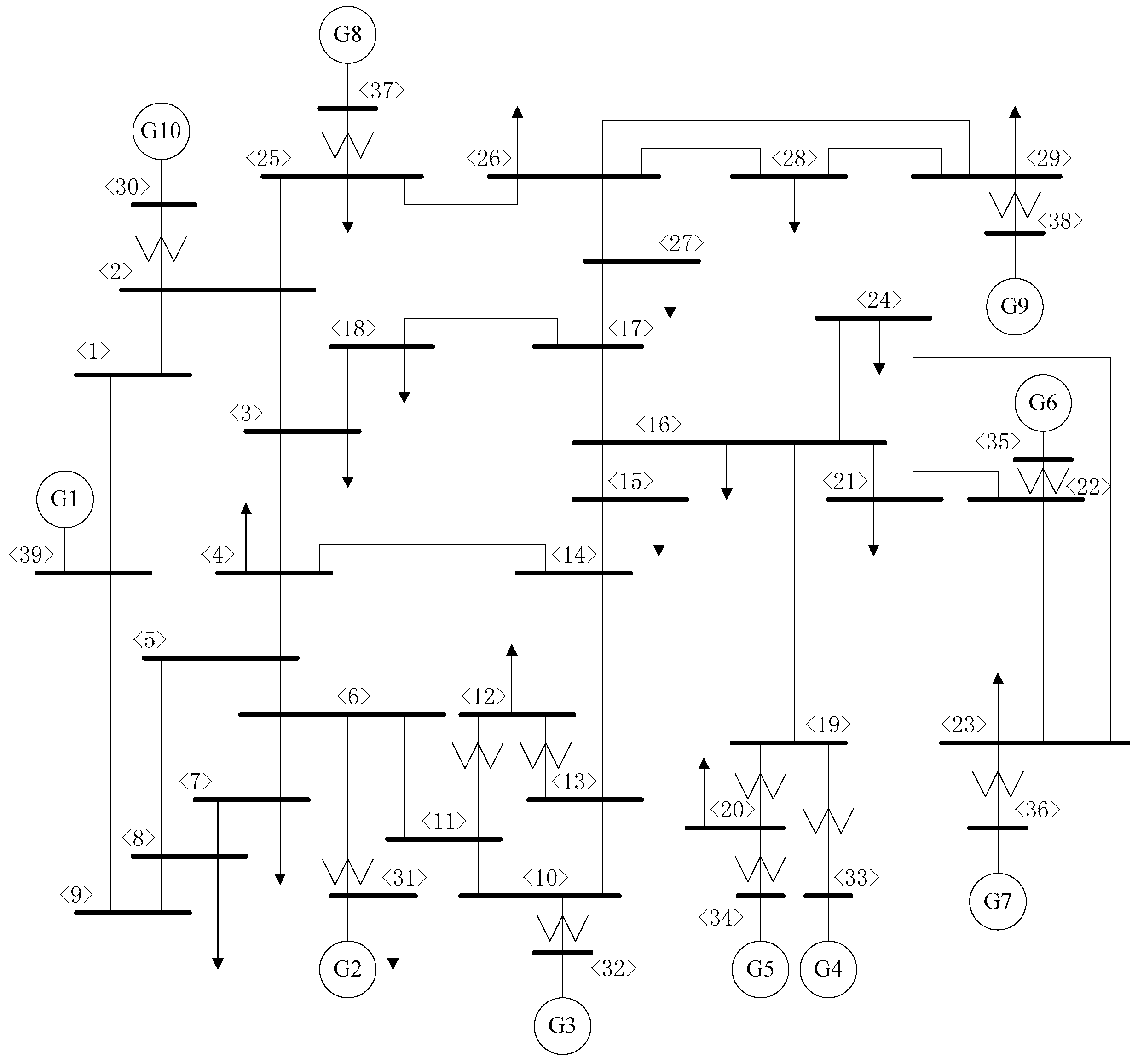
3.1. Database Generation

To evaluate the performance of the proposed transient stability prediction method, a New England 39-bus system is used. The diagram of the system is shown in Figure 4.
The data required to train the classifier are generated through offline dynamic simulations using the power system analysis software package (PSASP) and the integrated power system analysis platform developed by China EPRI [36]. The contingencies consider four fault types (LG, LL, LLG, LLL) in three locations (at 10%, 50% and 90% of the length) on each transmission line. The fault duration time is set to 0.08 s, 0.1 s, 0.12 s, 0.14 s, and 0.16 s for all the contingencies. Considering the action of backup protection, additional fault clearing times are considered, such as 0.2 s, 0.24 s, 0.28 s, and 0.32 s. All faults are cleared by opening the faulty line. The above contingencies are repeated at the base load level. The system has 34 transmission lines in total, so 3672 simulation cases are generated. In addition, different load levels (base load minus 20% and 10%, and base load plus 10% and 20%) are considered, and two random transmission lines are assumed to be faulted under each load level to generate an additional 864 cases. Thus, a total of 4536 simulation cases are generated, and for each case, the post-contingency variation of the generator voltage magnitude and rotor angle are recorded. All the simulation cases are used as training and testing data. A class label is assigned to each case according to the index set in PSASP. For each case, the simulation is performed for three seconds. If the difference between any two generator rotor angles exceeds 360° at the end of the simulation, then this case is assigned as “unstable”, and the corresponding label is “−1”. Otherwise, the case is stable, and the corresponding label is “+1”.

3.2. Training and Testing Datasets

The training and testing datasets are described in this section. Two training datasets are used to construct the proposed SVM models for rotor angle and voltage magnitude inputs. These datasets are obtained from the simulation cases described in Part 3.1. The number of cases in the training and testing sets is determined according to the proportion of the two kinds of samples. There are 3447 stable cases and 1089 unstable cases. Thus, we randomly select 2619 stable samples and 828 unstable samples to form the training set; the remaining 828 stable samples and 261 unstable samples are used as the testing set. There are two main parts in the Results section. In the first part, the proposed GTCFS feature selection approach is presented based on the basic database, which contains all 4536 samples. In the second part, to evaluate the proposed SVM model, some testing datasets are generated to validate the generalization capability of the proposed approach in transient stability prediction.

3.3. Feature Extraction, Selection and Test Results

The database contains all 4 fault types. Thirty consecutive samples (0.5 s) of each generator rotor angle and voltage magnitude after fault clearing were recorded for the SVM inputs. There are 3447 stable cases and 1089 unstable cases that contain all fault types. The training and testing cases are randomly chosen from the whole database, and the proportion is consistent with the two classes. Therefore, there are 2619 stable cases and 828 unstable cases in the training data, and the testing data have 828 stable cases and 261 unstable cases. Then, 27 trajectory cluster features (shown in Table 1) are calculated in the feature extraction stage. The data obtained from this process are normalized in the interval [0, 1] for the application of the proposed approach.

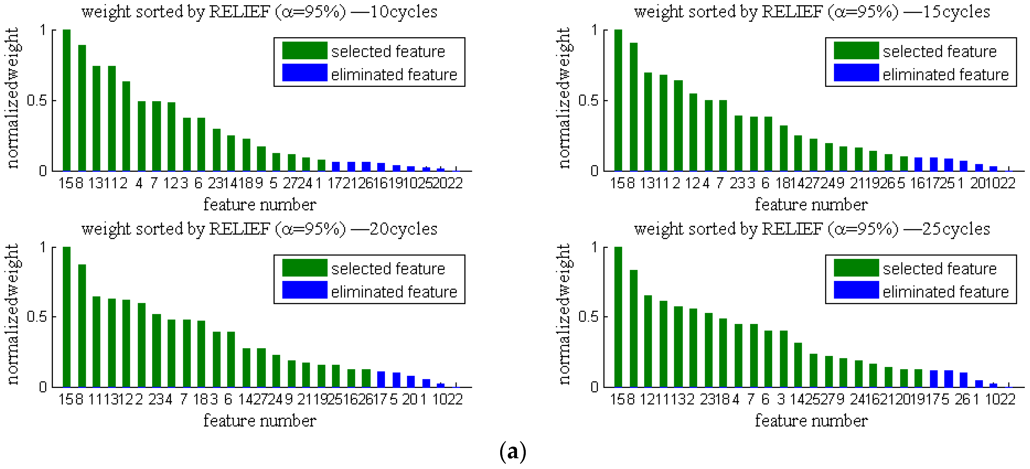
3.3.1. Filter Feature Selection Procedure

As mentioned above, we want to determine the minimum number of input vectors used for the classifier for computational efficiency, while maximizing the amount of key information. Therefore, we focus on two aspects: the number of sampling cycles and the number of features in the subset. First, to investigate the effectiveness of different scales of input data in the feature selection procedure, several time scales of input sampling data are considered: 10 cycles to 25 cycles in increments of one cycle. Then, the feature selection results are systematically analyzed. Moreover, experiments are conducted to determine the difference between using rotor angles and voltage magnitudes as the input variables.
First, the threshold τ in Algorithm 1 here is set according to statistical experience. By applying the RELIEF algorithm, a ranking of weights of the 27 features in ascending order is obtained. Then, the values are normalized to [0, 1]. Based on the concept of confidence intervals in statistics, a 95% confidence level represents a high probability event. Thus, the weight value represents the amount of information that a certain feature contains among the whole feature set. Then, if the cumulative proportion of the weight value that some features contain reaches 95%, these features possess the maximum “information” of the whole feature set. These mentioned features can be considered the most important features. Figure 5 shows that the green highlighted bars represent the feature weights that account for up to 95% of the whole cumulative weight values.
According to this hypothesis, the threshold τ is obtained as follows: the normalized weight values, which are sorted in descending order, are cumulatively summed. Meanwhile, the proportion of the cumulative value in all the weight values is calculated, and the calculation is stopped when the proportion reaches 95%. The weight of the features calculated using the RELIEF algorithm represents the degree of importance of the feature; thus, the cumulated features can be considered to be more important than all the features and the threshold τ is the corresponding normalized weight value when the cumulative calculation is stopped. For simplicity, only four cases, 10, 15, 20 and 25 cycles of sampling data are shown in Figure 5.
Figure 5 shows that there are many features in the candidate subsets after using the RELIEF algorithm, which might cause difficulties when establishing a classifier model. Therefore, the candidate subsets are further decreased. The AUC evaluation method is used to determine the optimal set of selected features. If we take a deeper look at Figure 5, it can be seen that the ranking of the selected features may change for different numbers of the sampling cycles. However, the features identified as the most relevant are nearly identical. The same result occurs for the voltage magnitudes. Thus, for a particular input variable, when the database is generated, the optimal set is uniform. In this study, we called this optimal set the GTCFS.

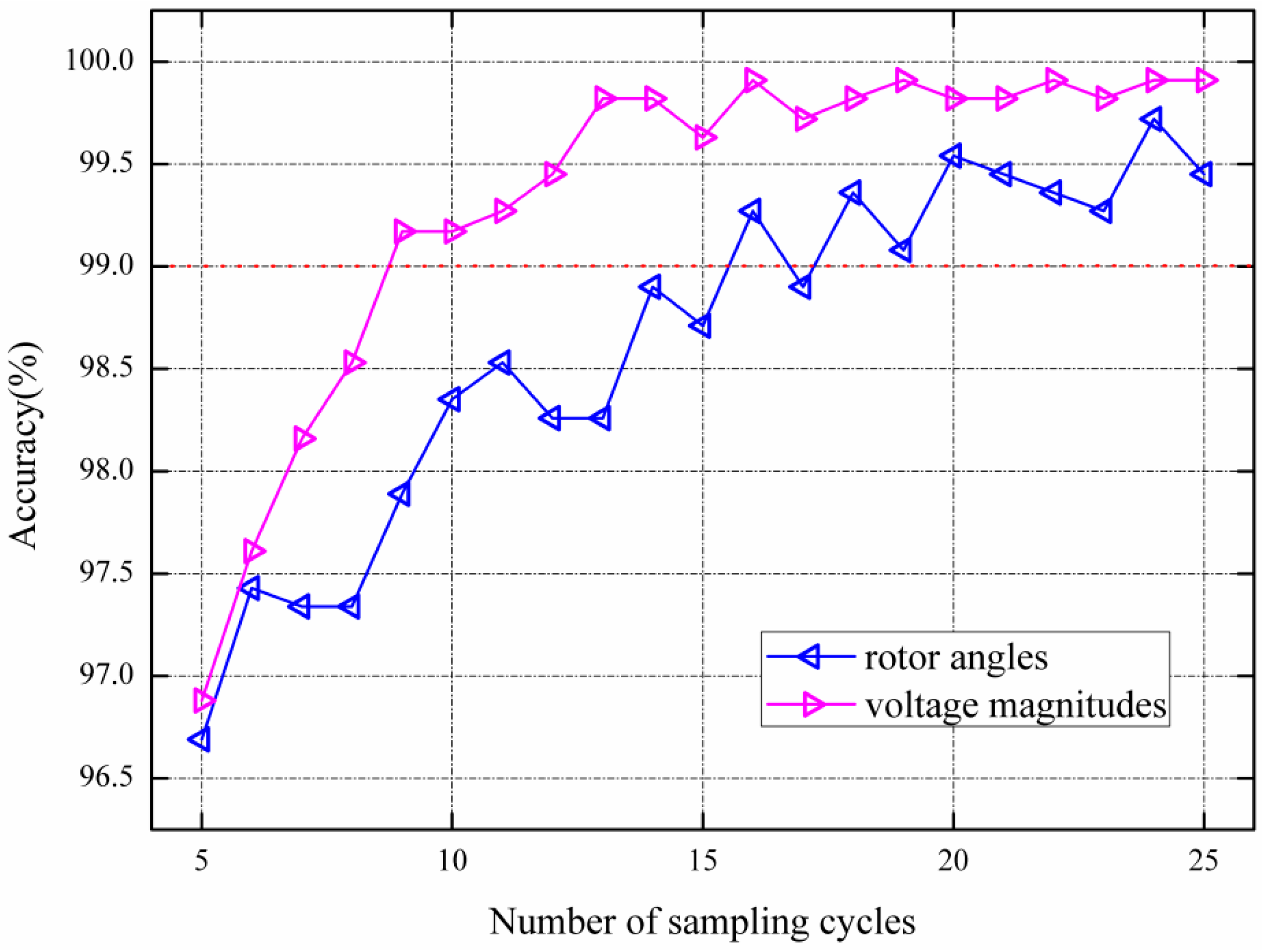
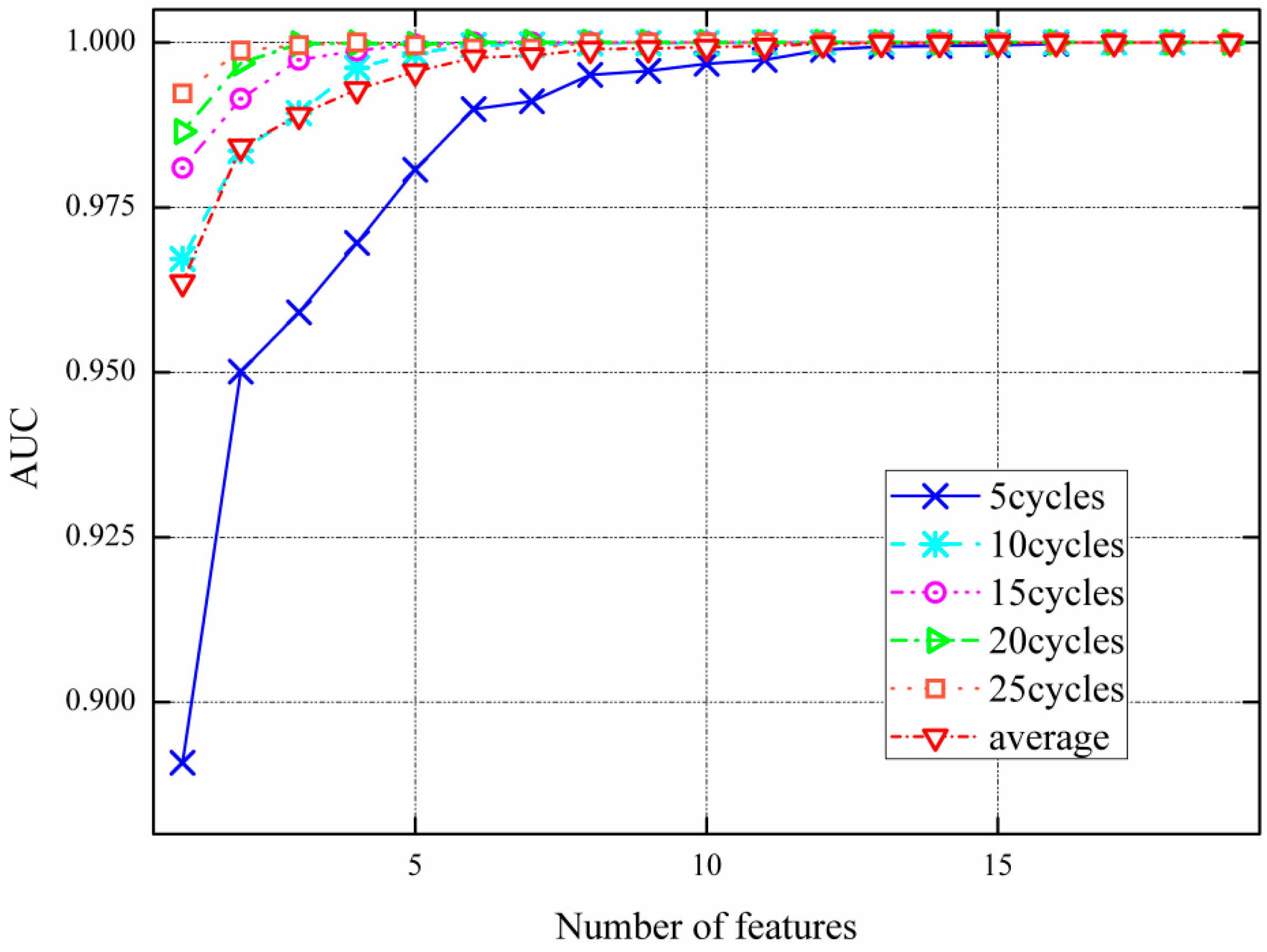
3.3.2. Wrapper Feature Selection Procedure

First, the multiple feature subsets of rotor angles are examined. The dataset is almost the same as the database shown in Figure 5. The only exception is that the sampling cycles examined here are 5, 10, 15 and 25. The candidate feature subsets reduced by the RELIEF algorithm are used as the inputs of the prediction model. Then, an ROC curve is drawn for the prediction mode. Each sampling cycle case corresponds to one stability status prediction result. The AUC statistics of the ROC curve are then obtained. By changing the number of features in the candidate subset, the variation in the AUC for different sampling cycles are shown in Figure 6.
Figure 6 shows that for all cases, AUC increases as the number of features grows. Once the feature number reaches eight, AUC shows minimal variations. In other words, the performance of the prediction model stops significantly improving beyond models trained with the eight most relevant features. Take the 25 cycles case for example; the first eight features are F15, F8, F12, F11, F13, F2, F23, and F18. Therefore, those eight features form the optimal subset of a certain database. For the TSA problem, these eight features form the GTCFS. Similar results are obtained for the voltage magnitudes. The AUC statistics are shown in Figure 7. If the rotor angles are used as the input vectors, the first “eight” features mostly contain “Envelope” and “Dispersion” features; in contrast, if the voltage magnitudes are used as the input vectors, most of the features are related to the “Arithmetic mean” and “Lower envelope”. The GTCFS is consistent with the transient stability phenomenon, namely, from the perspective of the rotor angle trajectories, when the variation of the clusters shows rapid divergence (reflected by a relatively large value of “Dispersion”), the system is unstable. From the perspective of the voltage magnitudes, when the voltage drop is sufficiently large and more difficult to recover (reflected by a relatively large value of “Lower envelope”), the system is unstable.
Furthermore, although the GTCFS is obtained, the scale of sampling cycles should also be considered. The models are trained using these 8 features, and the performance of the classifiers can be evaluated using two indexes: accuracy and AUC. More simulation results are shown in Figure 8.
Figure 8 shows that the prediction accuracy increases as the scale of sampling cycles grows, and both are similar for the two different input variables. While it is clear that the voltage magnitudes perform better than the rotor angles, for the voltage magnitudes, the accuracy remains at approximately 99% with little improvement when the number of the sampling cycles increases to nine. However, for rotor angles, the accuracy increases to greater than 99% as the number of sampling cycles increases to sixteen. Therefore, based on the calculated GTCFS, 9 cycles of voltage magnitude data could be used as the input vectors for the prediction model; in contrast, if rotor angles are used as the input variables, at least 16 cycles should be used.
To determine whether the trained SVM models with 8 optimal features are similar to those with 27 features, we use the accuracy and AUC to evaluate the SVM confidence score for four random subdivisions of the reference dataset. Each subdivision is the same size as the datasets mentioned above, that is, there are 3447 cases for the training sets and 1089 cases for the testing sets. The results are listed in Table 2. The whole dataset contains of 25 cycles. The proposed GTCFSs for a certain scale of sampling data have similar classification performance to the complete dataset. This reduction in the number of features and sampling cycles results in significant savings of computation burden, memory, and other requirements, which means the generated model shows desirable performance.
For each experiment, the time costs of computation are recorded simultaneously. The computational time can be divided into four parts: time for dataset preprocessing, time for feature extraction, time for feature selection and time for SVM model construction and validation. For simplicity, these consecutive process times are named T1, T2, T3 and T4. The results are shown in Table 3 and Table 4, which show that for the rotor angles cases, the processing time for the total dataset is 34.19 seconds, while for GTCFS, it is 30.52 seconds, 11% computation time reduction. For the voltage magnitudes cases, the processing time for the total dataset is 86.24 seconds and 23.93 seconds for GTCFS, a 72% reduction in computation time. If the proposed GTCFS-based method is applied to a large power system consisting of hundreds of generators and thousands of buses, the processing time would be reduced by a substantial amount.

3.4. Model Generalization Performance

3.4.1. Impact of Topology Changes

To verify the robustness of the proposed approach, the prediction method is tested under several topology changes. Three scenarios are considered: (1) The transmission line between Bus 3 and Bus 18 is out of service; (2) The transmission line between Bus 22 and Bus 23 is out of service; and (3) The transmission line between Bus 25 and Bus 26 is out of service. The contingencies considered are the most serious fault and three-phase to ground fault at 50% of the length of each transmission line. The fault duration times are 0.08 s, 0.1 s, 0.12 s, 0.14 s, and 0.16 s (approximately 5 to 10 cycles) for all contingencies. All cases are performed under the base load conditions. Therefore, a total of 165 cases are generated for each situation. Each situation forms one test set, and the training set is the previous 4536 simulation cases. We test the proposed approach using the rotor angles and voltage magnitudes. The two input variables are computed in parallel, and the better model performance is used as the final result. The test results are shown in Table 5.
All three prediction accuracies exceed 95%. The AUC statistics remain at a relatively high level. If the amount of historical data is sufficiently large, based on repeated experiments, the ideal prediction accuracy can exceed 98%. Therefore, the proposed method can successfully predict the transient stability even when the network topology is changed.

3.4.2. Impact of Load Level Changes

Taking the 3672 sampling data at the base load level as the training set, the other four load level scenarios are taken as the testing sets (80%, 90%, 110% and 120% of the base load level). There are 216 cases for each scenario. The model performances are listed in Table 6. The test results indicate that the proposed algorithm has good generalization ability for transient stability prediction under unknown and untrained load level conditions.
Close inspection of Table 5 and Table 6 shows that the proposed approach has strong generalization ability for transient stability prediction for unknown and untrained topologies and load levels, and not all the online contingency models have to be obtained. GTCFS can represent the global characteristics of the trajectory clusters of large disturbances in the system. Therefore, the proposed algorithm is robust, is not constrained by the trained topological structure and load levels of the network, and does not suffer from heavy relearning pressure.

3.4.3. Prediction Based on Incomplete WAMS Information

The WAMS system transmits real-time information from the generator to the system dispatch center, which requires the support of a wide-area high-speed communication system. Therefore, in practice, due to a malfunction in the communication channel, the time-domain response information may be incomplete. In previous studies, transient stability prediction based on all generator information can fail under these conditions. In this paper, even if some of the generator information is missing, the global trajectory cluster features can be recalculated. Some tests have been conducted under conditions of incomplete WAMS. To simulate the case of incomplete information, we assume that one or more trajectories in the test sets are randomly missing. The proposed predicting model performance is carefully examined under these circumstances. The database utilized here is the same as was used in Table 2. The test results are shown in Table 7.
Table 7 shows that if part of the generator information is missing, the prediction model performance is still satisfactory. The accuracies are all greater than 97% when information is missing from less than 5 generators. Thus, in practice, the proposed transient stability prediction method could maintain perfect performance as long as the key generators’ information is obtained. Therefore, the proposed method has the advantage when incomplete WAMS information is available, and it significantly improves the robustness of the transient stability prediction model.

4. Conclusions

In this paper, a data-mining technique is proposed to predict power system transient stability. First, trajectory cluster features are defined and extracted from the generator’s post-fault rotor angle and voltage magnitude trajectories. A hybrid filter-wrapper feature selection approach is designed to determine the most relevant features among the 27 initial candidates using the RELIEF algorithm. Through this approach, 8 cluster features are identified as the most important to construct an RBF-SVM classifier with a confidence score for the simulation dataset. The ROC analysis showed that the SVM models trained with the 8 proposed features have similar behavior to those trained with the complete set of features. This reduction in the number of required features can lead to important savings in preprocessing time, memory, and other computational requirements, independent of the system scale, which is important in real-time TSA. Finally, to evaluate our approach, we analyzed the generalizability of the SVM model trained using the proposed GTCFS for a collection of several unknown circumstances. The proposed stability classifier based on SVM and GTCFS shows excellent prediction accuracy with high computation efficiency, strong generalization ability to unknown load levels and topologies, independent of the system scale, and great robustness to incomplete WAMS information. However, this paper mainly focuses on the relevant feature extraction using a binary SVM model. In the near future, multi-category techniques should be studied to improve the prediction accuracy under critical stability cases, and the stability degree information should also be obtained.

Acknowledgments

This work was supported by the National Natural Science Foundation of China, Grant No. 51577009.

Author Contributions

Junyong Wu and Liangliang Hao conceived the structure and research direction of the paper; Yanzhen Zhou analyzed the data; Luyu Ji wrote the paper and completed the simulation for the case studies.

Conflicts of Interest

The authors declare no conflicts of interest.

References

  1. Pai, M.A. Energy Function Analysis for Power System Stability; Kluwer: Boston, MA, USA, 1989. [Google Scholar]
  2. Xue, Y.; Wehenkel, L.; Belhomme, R.; Rousseaux, P.; Pavella, M.; Euxibie, E. Extended equal area criterion revisited. IEEE Trans. Power Syst. 1992, 7, 1012–1022. [Google Scholar] [CrossRef]
  3. Wahab, N.I.A.; Mohamed, A.; Hussain, A. Fast transient stability assessment of large power system using probabilistic neural network with feature reduction techniques. Expert Syst. Appl. 2011, 38, 11112–11119. [Google Scholar] [CrossRef]
  4. Sharifian, A.; Sharifian, S. A new power system transient stability assessment method based on Type-2 fuzzy neural network estimation. Electr. Power Energy Syst. 2015, 64, 71–87. [Google Scholar] [CrossRef]
  5. Verma, K.; Niazi, K.R. Rotor Trajectory Index for Transient Security Assessment using Radial Basis Function Neural Network. In Proceedings of the IEEE PES Meeting, National Harbor, MD, USA, 27–31 July 2014; pp. 1–5.
  6. Haidar, A.M.A.; Mustafa, M.W.; Ibrahim, F.A.F.; Ibrahim, A.A. Transient stability evaluation of electrical power system using generalized regression neural networks. Appl. Soft Comput. 2011, 11, 3558–3570. [Google Scholar] [CrossRef]
  7. Rovnyak, S.M.; Taylor, C.W.; Sheng, Y. Decision trees using apparent resistance to detect impending loss of synchronism. IEEE Trans. Power Deliv. 2000, 15, 1157–1162. [Google Scholar] [CrossRef]
  8. Gao, Q.; Rovnyak, S.M. Decision trees using synchronized phasor measurements for wide-area response-based control. IEEE Trans. Power Syst. 2011, 26, 855–861. [Google Scholar] [CrossRef]
  9. Dong, Z.Y.; Xu, Y.; Zhang, P.; Wong, K.P. Using IS to Assess an Electric Power System’s Real-Time Stability. IEEE Intell. Syst. 2013, 28, 60–66. [Google Scholar] [CrossRef]
  10. Bahbah, A.G.; Girgis, A.A. New method for generators’ angles and angular velocities prediction for transient stability assessment of multimachine power systems using recurrent artificial neural network. IEEE Trans. Power Syst. 2004, 19, 1015–1022. [Google Scholar] [CrossRef]
  11. Karami, A.; Esmaili, S.Z. Transient stability assessment of power systems described with detailed models using neural network. Int. J. Electr. Power Energy Syst. 2013, 45, 279–292. [Google Scholar] [CrossRef]
  12. Sulistiawati, I.B.; Priyadi, A.; Qudsi, O.A.; Soeprijanto, A.; Yorino, N. Critical Clearing Time prediction within various loads for transient stability assessment by means of the Extreme Learning Machine method. Int. J. Electr. Power Energy Syst. 2016, 77, 345–352. [Google Scholar] [CrossRef]
  13. Li, Y.; Li, G.Q.; Wang, Z.H. A Multifeature Fusion Approach for Power System Transient Stability Assessment Using PMU Data. Math. Probl. Eng. 2015, 6, 1–10. [Google Scholar] [CrossRef]
  14. Haykin, S. Neural Networks: A Comprehensive Foundation, 2nd ed.; Prentice-Hall: Upper Saddle River, NJ, USA, 1999. [Google Scholar]
  15. Tsoa, S.K.; Gu, X.P. Feature selection by separability assessment of input spaces for transient stability classification based on neural networks. Int. J. Electr. Power Energy Syst. 2004, 26, 153–162. [Google Scholar] [CrossRef]
  16. Sawhney, H.; Jeyasurya, B. A feed-forward artificial neural network with enhanced feature selection for power system transient stability assessment. Electr. Power Syst. Res. 2006, 76, 1047–1054. [Google Scholar] [CrossRef]
  17. Rajapakse, A.D.; Gomez, F.R.; Nanayakkara, K.; Crossley, P.A.; Terzija, V.T. Rotor angle instability prediction using post-disturbance voltage trajectories. IEEE Trans. Power Syst. 2010, 25, 947–956. [Google Scholar] [CrossRef]
  18. Gomez, F.R.; Rajapakse, A.D.; Annakkage, U.; Fernando, I. Support vector machine-based algorithm for post-fault transient stability status prediction using synchronized measurements. IEEE Trans. Power Syst. 2011, 26, 1474–1483. [Google Scholar] [CrossRef]
  19. Guo, T.Y.; Milanović, J.V. Online Identification of Power System Dynamic Signature Using PMU Measurements and Data Mining. IEEE Trans. Power Syst. 2016, 31, 1760–1768. [Google Scholar] [CrossRef]
  20. Gomez, F.R.; Rajapakse, A.D.; Annakkage, U. Transient stability prediction algorithm based on post-fault recovery voltage measurements. In Proceedings of the 2009 IEEE Electrical Power & Energy Conference (EPEC), Montreal, QC, Canada, 22–23 October 2009; pp. 1–6.
  21. Zhao, J.Q.; Li, J.; Wu, X.C.; Men, K.; Hong, C.; Liu, Y.J. A novel real-time transient stability prediction method based on post-disturbance voltage trajectories. In Proceedings of the International Conference on Advanced Power System Automation and Protection (APAP), Beijing, China, 16–20 October 2011; pp. 730–736.
  22. Gu, X.P.; Li, Y.; Jia, J.H. Feature selection for transient stability assessment based on kernelized fuzzy rough sets and memetic algorithm. Int. J. Electr. Power Energy Syst. 2015, 64, 664–670. [Google Scholar] [CrossRef]
  23. Kira, K.; Rendell, L.A. A practical approach to feature selection. In Proceedings of the Ninth International Workshop on Machine Learning, San Jose, CA, USA, 12–16 July 1992; Morgan Kaufmann Publishers Inc.: Aberdeen, Scotland, UK, 1992; pp. 249–256. [Google Scholar]
  24. Fawcett, T. An introduction to ROC analysis. Pattern Recognit. Lett. 2006, 27, 861–874. [Google Scholar] [CrossRef]
  25. Block, P.; Paern, J.; Hüllermeier, E.; Sanschagrin, P.; Sotriffer, C.A. Physicochemical descriptors to discriminate protein–protein interactions in permanent and transient complexes selected by means of machine learning algorithms. Proteins Struct. Funct. Bioinform. 2006, 65, 607–622. [Google Scholar] [CrossRef] [PubMed]
  26. Mizianty, M.; Kurgan, L. Modular prediction of protein structural classes from sequences of twilight-zone identity with predicting sequences. BMC Bioinform. 2009, 10, 414. [Google Scholar] [CrossRef] [PubMed]
  27. Cortes, C.; Vapnik, V. Support Vector Networks. Available online: http://citeseerx.ist.psu.edu/viewdoc/summary?doi=10.1.1.15.9362&rank=3 (accessed on 8 October 2016).
  28. Herrera, L.; Pomares, H.; Rojas, I.; Guillén, A.; Prieto, A.; Valenzuela, O. Recursive prediction for long term time series forecasting using advanced models. Neurocomputing 2007, 70, 2870–2880. [Google Scholar] [CrossRef]
  29. Chang, C.C.; Lin, C.J. LIBSVM: A Library for Support Vector Machines. 2001. Available online: http://www.csie.ntu.edu.tw/~cjlin/libsvm (accessed on 8 October 2016).
  30. Suykens, J.A.K.; Gestel, T.V.; Brabanter, J.D.; Moor, B.D.; Vandewalle, J. Least Squares Support Vector Machines; World Scientific Publishing Company: Singapore, 2003. [Google Scholar]
  31. Wu, T.; Lin, C.; Weng, R.C. Probability estimates for multi-class classification by pairwise coupling. J. Mach. Learn. Res. 2004, 5, 975–1005. [Google Scholar]
  32. Zhang, T. Statistical behaviour and consistency of classification methods based on convex risk minimization. Ann. Stat. 2004, 32, 56–134. [Google Scholar] [CrossRef]
  33. Chen, X.W.; Wasikowski, M. FAST: A roc-based feature selection metric for small samples and imbalanced data classification problems. In Proceedings of the 14th ACM SIGKDD International Conference on Knowledge Discovery and Data Mining, New York, NY, USA, 24–27 August 2008; pp. 124–132.
  34. Alshawabkeh, M.; Aslam, J.A.; Dy, J.; Kaeli, D. Feature Selection Metric Using AUC Margin for Small Samples and Imbalanced Data Classification Problems. IEEE Comput. Soc. 2011, 1, 145–150. [Google Scholar]
  35. Krawczyk, B.; Woźniak, M.; Herrera, F. Weighted one-class classification for different types of minority class examples in imbalanced data. In Proceedings of the 2014 IEEE Computational Intelligence and Data Mining (CIDM), Orlando, FL, USA, 9–12 December 2014; pp. 337–344.
  36. Wu, Z.X.; Zhou, X.X. Power system analysis software package (PSASP)—An integrated power system analysis tool. In Proceedings of the 1998 International Conference POWERCON, Beijing, China, 18–21 August 1998; pp. 7–11.
Figure 1. Time-domain trajectories, (a) Whole information; (b) Without Generator 7 and Generator 10.
Energies 09 00898 g001
Figure 2. Variation of the trajectory dispersion, (a) Whole information; (b) Without Generator 7 and Generator 10.
Energies 09 00898 g002
Figure 3. Transient stability prediction algorithm flowchart based on trajectory cluster features.
Energies 09 00898 g003
Figure 4. Diagram of the New England 39-bus test system.
Energies 09 00898 g004
Figure 5. Normalized weight rankings of the features obtained by RELIEF (range [0, 1]) for different sampling cycles. (a) Rotor Angle; (b) Voltage Magnitude.
Energies 09 00898 g005aEnergies 09 00898 g005b
Figure 6. AUC for the rotor angles feature subset.
Energies 09 00898 g006
Figure 7. AUC for the voltage magnitudes feature subset.
Energies 09 00898 g007
Figure 8. Accuracy variation for different sampling cycles.
Energies 09 00898 g008
Table 1. Description of the 27 extracted trajectory cluster features.
No.DescriptionNo.Description
F1Arithmetic meanF15Gradient of the envelope height
F2Degree of dispersionF16Trajectory curvature
F3Upper envelopeF17Curvature of the arithmetic mean
F4Lower envelopeF18Curvature of dispersion
F5Mid-rangeF19Curvature of the upper envelope
F6Difference between the upper envelope and arithmetic meanF20Curvature of the lower envelope
F7Difference between the lower envelope and arithmetic meanF21Curvature of the mid-range
F8Envelope heightF22Arithmetic mean variation acceleration
F9Difference between the arithmetic mean and mid-rangeF23Dispersion variation acceleration
F10Gradient of the arithmetic meanF24Upper envelope acceleration
F11Gradient of dispersionF25Lower envelope acceleration
F12Gradient of the upper envelope F26Mid-range variation acceleration
F13Gradient of the lower envelope F27Envelope height variation acceleration
F14Gradient of the arithmetic mean--
Table 2. Results for the accuracy and area under the ROC curve (AUC).
Training and Test GroupRotor AnglesVoltage Magnitudes
GTCFS SetTotal Feature SetGTCFS SetTotal Feature Set
Acc 1(%)AUCAcc (%)AUCAcc (%)AUCAcc (%)AUC
1st98.350.999100199.080.99981001
2nd98.440.998999.360.9997
3rd98.710.99998.990.9997
4th98.260.999298.900.9996
Mean98.440.99999.080.9997
1 Acc: Accuracy.
Table 3. Processing time for the total dataset.
Training and Test GroupRotor AnglesVoltage Magnitudes
T1T2T3T4SumT1T2T3T4Sum
1st0.055.93-28.0734.050.045.97-80.8386.85
2nd0.056.25-26.9533.240.055.88-80.2786.20
3rd0.056.03-28.0034.080.056.18-79.1985.42
4th0.056.09-29.2435.380.046.07-80.4086.51
Mean0.056.08-28.0734.190.056.03-80.1786.24
Note: There are no feature selection procedures for total the dataset; Units: seconds.
Table 4. Processing time for the GTCFS set.
Training and Test GroupRotor AnglesVoltage Magnitudes
T1T2T3T4SumT1T2T3T4Sum
1st0.054.5721.333.5429.480.043.1815.505.1123.83
2nd0.054.5620.513.3528.460.043.3615.775.1724.34
3rd0.044.5424.303.7432.630.043.3115.775.1624.28
4th0.044.4723.703.3031.510.043.3814.685.1623.26
Mean0.054.5422.463.4830.520.043.3115.435.1523.93
Units: seconds.
Table 5. Results of the prediction effect for unknown topology.
ScenariosStable Case NumberUnstable Case NumberPrediction Accuracy (%)AUC
ActualPredictedActualPredicted
Scenario 1141141242298.790.9994
Scenario 2127126383295.760.9758
Scenario 3127127383296.360.9816
Table 6. Results of the prediction effect for an unknown load level.
Load LevelPrediction Accuracy (%)AUC
80%93.520.9999
90%99.070.9997
110%90.740.9978
120%81.010.9901
Table 7. Statistics of the prediction for incomplete WAMS information.
Missing Number of GeneratorsStable Case NumberUnstable Case NumberPrediction Accuracy (%)AUC
ActualPredictedActualPredicted
082882526124998.620.9961
182882526124798.430.9948
282882326124397.890.9943
382882026124597.780.9942
482882126124597.890.9955
582881926124297.430.9931

