A Rest Time-Based Prognostic Framework for State of Health Estimation of Lithium-Ion Batteries with Regeneration Phenomena

Abstract

State of health (SOH) prognostics is significant for safe and reliable usage of lithium-ion batteries. To accurately predict regeneration phenomena and improve long-term prediction performance of battery SOH, this paper proposes a rest time-based prognostic framework (RTPF) in which the beginning time interval of two adjacent cycles is adopted to reflect the rest time. In this framework, SOH values of regeneration cycles, the number of cycles in regeneration regions and global degradation trends are extracted from raw SOH time series and predicted respectively, and then the three sets of prediction results are integrated to calculate the final overall SOH prediction values. Regeneration phenomena can be found by support vector machine and hyperplane shift (SVM-HS) model by detecting long beginning time intervals. Gaussian process (GP) model is utilized to predict the global degradation trend, and nonlinear models are utilized to predict the regeneration amplitude and the cycle number of each regeneration region. The proposed framework is validated through experimental data from the degradation tests of lithium-ion batteries. The results demonstrate that both the global degradation trend and the regeneration phenomena of the testing batteries can be well predicted. Moreover, compared with the published methods, more accurate SOH prediction results can be obtained under this framework.

1. Introduction

Lithium-ion batteries have attracted significant attention for many more energy or power demanding applications such as in consumer electronics, aerospace, hybrid and electric vehicles and smart grids applications, due to their superior energy density and high specific energy over other rechargeable battery technologies [1]. To reduce the maintenance costs and the chances of failure as well as improve the safety and reliability of systems, battery degradation, prognostics and maintenance optimization have attracted much attention among researchers in the fields of energy, reliability engineering and aerospace engineering [2,3,4]. Also, state of health (SOH) prognostics of lithium-ion battery has become a key factor that helps fulfill intelligent battery management [5,6,7].

Traditionally, prognostics can be implemented by using either physics-based approaches or data-driven approaches [8]. However, as capacity fade phenomenon is the result of various processes and their interactions, such as chemical side reactions or loss of conductivity [9,10,11], it is difficult to monitor the internal state of a battery in real time and obtain an accurate physics-based model. By contrast, data-driven approaches can achieve health state assessment and prognostics based only on monitoring parameters and testing data samples. As a result, data-driven techniques draw more and more attention in SOH prognostics. In the literature, statistical, computational and artificial intelligence algorithms, such as autoregressive model [12], particle filter (PF) [13,14], Gaussian process regression [15], Wiener process [16], relevance vector machine (RVM) [17], Bayesian approach [18], support vector machine (SVM) [19] and neural networks [20,21] have been used for battery SOH and remaining useful life (RUL) prognostics in various applications. Capacity fade and impedance increase are the two most used health indicators of batteries. Because capacity is available for monitoring online with low costs, it is widely used in battery health management systems. However, the existence of capacity regeneration phenomena remains a big challenge for prognostics.

Researchers have recognized that reaction products in batteries have a chance to dissipate during the rest time and this phenomenon leads to charge regeneration (or self-recharge). Some researchers have approximately described the law of capacity regeneration by the empirical model of charge regeneration [16,22,23]. However, the mechanisms of charge regeneration and capacity regeneration may be quite different. The self-recharge phenomenon just needs about 10 min to become steady, while capacity regeneration takes around 2 h of rest-time to appear [24]. Therefore, the short relaxation of 10 min will not lead to the increase of battery capacity. Some researchers have assumed that capacity regeneration has certain regularity over time [24]. Liu et al. [15] has predicted SOH regeneration and degradation by using combination Gaussian progress function regression. He et al. [25] has decoupled local regeneration and global degradation with wavelet and predicted them respectively. However, the capacity regeneration phenomenon is strongly related to the rest time which is determined by practical application demands of the battery [24]. Therefore, without considering the rest time of the battery, it is hard to predict regeneration phenomenon accurately. Some researchers have treated the capacity regeneration as uncertainty (unpredictable disturbance). Olivares et al. [26] and Orchard et al. [27] have provided some approaches to detect the regeneration phenomenon and predicted SOH by isolating the effects of regeneration. Qin et al. [28] has predicted the global degradation trend directly using the raw SOH data by improving the robustness of a prediction algorithm. Li et al. [29] has utilized the history data of the same type of batteries and indirectly considered the influence of regeneration on battery aging. Although these approaches can capture and predict the global degradation trend of batteries, they have failed to predict the regeneration phenomenon. Therefore, the SOH prediction errors around these related cycles are large. In recent years, although it has been noted that there is a close relationship between the regeneration phenomenon and the rest time [16,24,30], no effective prediction approach that uses the rest time to take regeneration into account has been found.

To address the regeneration phenomenon prediction problem, this paper proposes a rest time-based prognostic framework (RTPF). This framework is composed of extraction phase, prediction phase, and integration phase. In extraction phase, SOH values of regeneration cycles and the number of cycles in regeneration regions and global degradation series are extracted from raw SOH data. After that, the above three series are predicted respectively in prediction phase. In integration phase, the three sets of prediction results are integrated to calculate the final SOH prediction values. Because there is an almost linear relationship between the cycle beginning time interval of two adjacent cycles and the pause time (rest time) during this period, the support vector machine and hyperplane shift (SVM-HS) model is proposed to detect long beginning time intervals to find obvious regeneration phenomena. Also, the Gaussian process (GP) model is used for the prediction of the global degradation trend. Nonlinear models are adopted to predict regeneration amplitude and the number of cycles in regeneration regions, respectively. Finally, the effectiveness of the proposed prognostic framework is validated by using the National Aeronautics and Space Administration (NASA) battery data sets. The results show that the future regeneration phenomena can be well predicted and compared with eight published methods, and more accurate SOH prediction results can be obtained by this framework.

The remainder of this paper is organized as follows: in Section 2, the related classification model and prediction model are introduced. The proposed RTPF is described in detail in Section 3. In Section 4, the effectiveness of the proposed framework is demonstrated via battery SOH prediction experiments. Finally, the conclusion is provided in Section 5.

2. Related Work

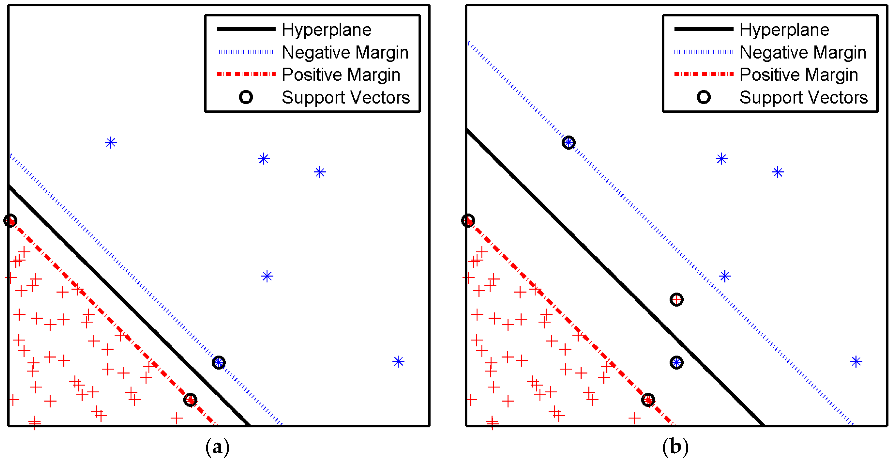
2.1. Support Vector Machine and Hyperplane Shift

2.1.1. Support Vector Machine

Let $S=\left\{\left({\mathit{x}}_i,y_i\right)|i=1,2,...,N\right\}$ be a two-class dataset, where ${\mathit{x}}_i\in {\text{ℝ}}^m$ are the data points and $y_i\in \left\{1,-1\right\}$ are the corresponding labels. These samples can be used to determine a decision function to separate two classes, which can be expressed by a linear boundary:

$$g\left({\mathit{x}}^{*}\right)=\mathrm{sgn}\left({\mathit{w}}^T{\mathit{x}}^{*}+b\right)$$

(1)

where $\mathit{w}\left(\mathit{w}\in {\text{ℝ}}^m\right)$ and $b\left(b\in \text{ℝ}\right)$ are decision coefficients obtained by learning from the dataset $S$. And ${\mathit{x}}^{*}$ is a new sample that need to be classified.

Hard margin SVM attempts to find the max-margin hyperplane ${\mathit{w}}^T\mathit{x}+b=0$. In this way, the points in the positive class have a positive margin and points in the negative class have a negative margin. The optimization problem can be expressed by:

$$\underset{\mathit{w},b}{\min }\frac{1}{2}{\Vert \mathit{w}\Vert }^2$$

(2a)

subject to:

$$y_i\left({\mathit{w}}^T{\mathit{x}}_i+b\right)\ge 1,\forall \left({\mathit{x}}_i,y_i\right)\in S$$

(2b)

Introducing Lagrange multipliers ${\alpha }_i$ corresponding to the constraints in Equation (2b), this optimization problem can be solved by using its dual problem counterpart [31].

$$\underset{\mathsf{\alpha }\in {\text{ℝ}}^N}{\min }\frac{1}{2}{\displaystyle \sum _{i=1}^N{\displaystyle \sum _{j=1}^N{y}_i}{y}_j{\alpha }_i{\alpha }_j{\mathit{x}}_i^T{\mathit{x}}_j}-{\displaystyle \sum _{i=1}^N{\alpha }_i}$$

(3a)

subject to:

$${\displaystyle \sum _{i=1}^N{y}_i{\alpha }_i=0}$$

(3b)

$${\alpha }_i\ge 0,i=1,2,...,N$$

(3c)

Because Equation (3) is a standard quadratic programming, the optimization problem can be easily solved, and then the decision coefficients can be obtained as follows:

$$\mathit{w}={\displaystyle \sum _{i=1}^N{y}_i{\alpha }_i{\mathit{x}}_i}={\displaystyle \sum _{{\alpha }_i>0}{y}_i{\alpha }_i{\mathit{x}}_i}$$

(4)

$$b=y_s-{\mathit{w}}^T{\mathit{x}}_s$$

(5)

where $\left({\mathit{x}}_s,y_s\right)$ is any support vector which is defined by the condition ${\alpha }_i>0$.

For the cases that two classes in the dataset are not linearly separable, the constraints are relaxed by introducing a slack variable ${\xi }_i$ for each data point. Then, the soft margin SVM optimization problem is as:

$$\underset{\mathit{w},b,\mathsf{\xi }}{\min }\frac{1}{2}{\Vert \mathit{w}\Vert }^2+C{\displaystyle \sum _{i=1}^N{\mathsf{\xi }}_i}$$

(6a)

subject to:

$$y_i\left({\mathit{w}}^T{\mathit{x}}_i+b\right)\ge 1-{\mathsf{\xi }}_i,\forall \left({\mathit{x}}_i,y_i\right)\in S$$

(6b)

$${\mathsf{\xi }}_i\ge 0,\forall \left({\mathit{x}}_i,y_i\right)\in S$$

(6c)

where $C$ is the penalty parameter, and ${\mathsf{\xi }}_i$ is the slack variable. The goal of large margin can be gotten by minimizing the term ${\Vert \mathit{w}\Vert }^2$ in the objective function, while the goal of small margin violations can be obtained by minimizing the term ${\displaystyle {\sum }_{i=1}^N{\mathsf{\xi }}_i}$. The parameter $C$ is defined by users’ large-margin favor or small-violations favor. Lagrange multipliers ${\alpha }_i$ are introduced for Equation (6b) and ${\mathsf{\beta }}_i$ are for Equation (6c). Then ${\mathsf{\beta }}_i$ can be removed by KKT condition ${\mathsf{\beta }}_i=C-{\alpha }_i$. The final dual expression of soft margin SVM is as follows:

$$\underset{\mathsf{\alpha }\in {\text{ℝ}}^N}{\min }\frac{1}{2}{\displaystyle \sum _{i=1}^N{\displaystyle \sum _{j=1}^N{y}_i}{y}_j{\alpha }_i{\alpha }_j{\mathit{x}}_i^T{\mathit{x}}_j}-{\displaystyle \sum _{i=1}^N{\alpha }_i}$$

(7a)

subject to:

$${\displaystyle \sum _{i=1}^N{y}_i{\alpha }_i=0}$$

(7b)

$$0\le {\alpha }_i\le C,i=1,2,...,N$$

(7c)

Decision coefficients can also be obtained by Equations (4) and (5), where $\left({\mathit{x}}_s,y_s\right)$ is any support vector which is defined by the condition $0<{\alpha }_i<C$. Moreover, it can be seen from Equations (3) and (7) that the only difference between the dual problem of hard margin SVM and the dual problem of soft margin SVM is the constraint $C$ on ${\alpha }_i$. This means that if the dataset is linearly separable, hard margin SVM can be obtained by setting a large penalty parameter $C$ in the soft margin SVM.

For any test vector ${\mathit{x}}^{*}$, the decision function of both hard margin SVM and soft margin SVM is finally given by:

$$g\left({\mathit{x}}^{*}\right)=\mathrm{sgn}\left({\displaystyle \sum _{{\alpha }_i>0}{y}_i{\alpha }_i{\mathit{x}}_i^T\mathit{x}+b}\right)$$

(8)

The Vapnik-Chervonenkis (VC) dimension is usually used to measure the complexity of a model. The VC dimension of SVM is bounded as follows [32]:

$$d_{VC\_SVM}\le \min \left(\left[R^2/M^2\right],d\right)+1$$

(9)

where $R$ is the smallest diameter which encloses all training sample, $d$ is the dimension of given training samples and $M$ is the margin. For general $d$ dimension classification models, the VC dimension is $\left(d+1\right)$. For example, the VC dimension of perceptron learning algorithm (PLA), one of the simplest classifiers in machine learning, is shown as follows [33]:

$$d_{VC\_PLA}=d+1$$

(10)

An advantage of SVM-HS method is that the complexity can be bounded by $\left[R^2/M^2\right]$ and does not explicitly depend on the dimension d.

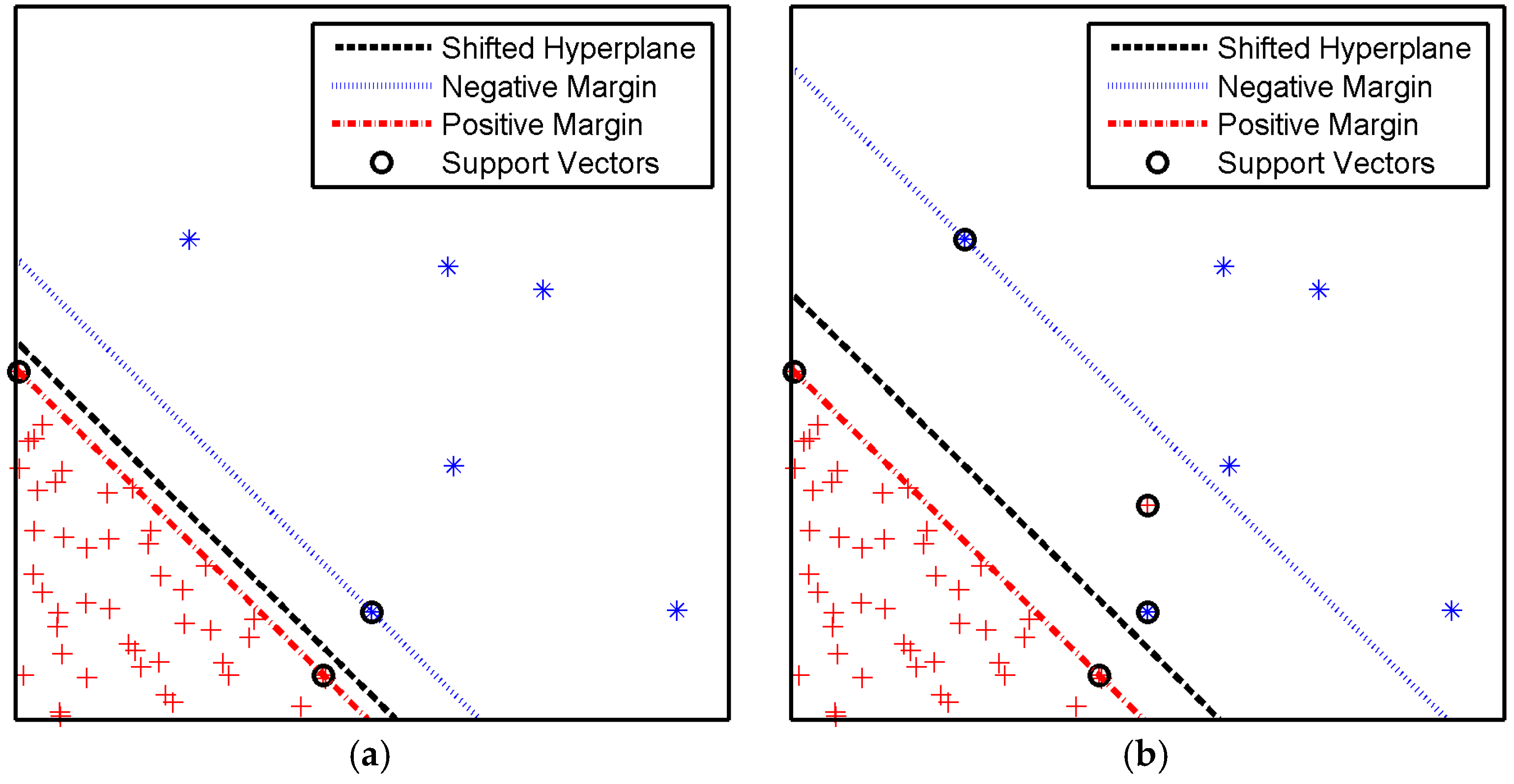
2.1.2. Hyperplane Shift

When the dataset is unbalanced, the majority class is likely to have more representatives. The noise of majority class may cause the SVM to move the separating hyperplane towards the minority class. The described effects are illustrated in Figure 1.

One approach to solving this problem is to shift the hyperplane. SVM can be trained in the traditional way, but the decision function given by Equation (8) is replaced by:

$$g\left({\mathit{x}}^{*}\right)=\mathrm{sgn}\left({\displaystyle \sum _{{\alpha }_i>0}{y}_i{\alpha }_i{\mathit{x}}_i^T\mathit{x}+b+p}\right)$$

(11)

where $p\in (-1,1)$ is the offset. The shift range is within the positive and negative margin bounds. The hyperplane is shifted towards positive data points when $p<0$, and towards negative data points when $p>0$. Also, the shifted hyperplane gives a larger margin for the minority class, and a smaller margin for the majority class. Moreover, the sum of positive and negative margin is unchanged, which means that the large margin principle of SVM is still effective. Because the offset parameter p is constant, the complexity of SVM-HS is the same as that of SVM. If the dataset is linearly separable, using hard margin SVM or soft margin SVM with large penalty parameter, the hyperplane shift has no effect on the accuracy of classification of all the data points. If the dataset is not linearly separable, using soft margin SVM with large penalty parameter, the shifted hyperplane is in the area of overlap. In this situation, the classification accuracy may be increased or decreased, because solving the optimization problem (Equation (6)) is to minimize the term ${\displaystyle {\sum }_{i=1}^N{\mathsf{\xi }}_i}$ instead of ${\displaystyle {\sum }_{i=1}^N〚y_i\ne \mathrm{sgn}\left({\mathit{w}}^T{\mathit{x}}_i+b\right)〛}$. Figure 2 shows the shift of hyperplane, where $p=-0.5$.

2.2. Gaussian Process Model

GP model is a flexible nonparametric model, which has been widely applied to multi-step-ahead predictions in time series analysis [25,34]. A GP model is completely specified by its mean function and covariance function. The mean function $m\left(\mathit{x}\right)$ and the covariance function $k\left(\mathit{x},{\mathit{x}}^{\prime }\right)$ of a real process $f\left(\mathit{x}\right)$ are as:

$$m\left(\mathit{x}\right)=E\left(f\left(\mathit{x}\right)\right)$$

(12)

$$k\left(\mathit{x},{\mathit{x}}^{\prime }\right)=\mathrm{cov}\left(f\left(\mathit{x}\right),f\left({\mathit{x}}^{\prime }\right)\right)=E\left[\left(f\left(\mathit{x}\right)-m\left(\mathit{x}\right)\right)\left(f\left({\mathit{x}}^{\prime }\right)-m\left({\mathit{x}}^{\prime }\right)\right)\right]$$

(13)

The regression function is denoted by:

$$f\left(\mathit{x}\right)~\mathrm{GP}\left(m\left(\mathit{x}\right),k\left(\mathit{x},{\mathit{x}}^{\prime }\right)\right)$$

(14)

It is common to utilize a mean function of $m\left(\mathit{x}\right)=0$, since the GP is flexible enough to model the mean arbitrarily well [35]. Also, the squared exponential covariance function applied in SOH prognostics is as follows:

$$k\left(\mathit{x},{\mathit{x}}^{\prime }\right)={\mathsf{\sigma }}_f^2\exp \left(-\frac{1}{2l^2}{\left(\mathit{x}-{\mathit{x}}^{\prime }\right)}^2\right)$$

(15)

where ${\mathsf{\sigma }}_f^2$ controls the vertical scale of this function, and $l$ is a length-scale parameter that governs the speed of the correlation decrease as the input data distance increases.

For training dataset $D=\left\{\left({\mathit{x}}_i,y_i\right)|i=1,2,...,N\right\}$, the target $y_i$ is described as:

$$y_i=f\left({\mathit{x}}_i\right)+{\mathsf{\epsilon }}_i,i=1,...,N$$

(16)

where ${\mathsf{\epsilon }}_i~N\left(0,{\mathsf{\sigma }}^2\right),i=1,...,N$. For a new test input ${\mathit{x}}^{*}$, the prior distribution for GP is as follows:

$$\left[\begin{array}{c}\mathit{y}\\ f^{*}\end{array}\right]~N\left(0,\left[\begin{array}{cc}\mathit{K}\left(\mathit{X},\mathit{X}\right)+{\sigma }_n^2\mathit{I}& {\mathit{k}}^T\left({\mathit{x}}^{*},\mathit{X}\right)\\ \mathit{k}\left({\mathit{x}}^{*},\mathit{X}\right)& k\left({\mathit{x}}^{*},{\mathit{x}}^{*}\right)\end{array}\right]\right)$$

(17)

where $\mathit{k}\left({\mathit{x}}^{*},\mathit{X}\right)=\left[k\left({\mathit{x}}^{*},{\mathit{x}}_1\right),k\left({\mathit{x}}^{*},{\mathit{x}}_2\right),...,k\left({\mathit{x}}^{*},{\mathit{x}}_N\right)\right]$. The posterior distribution for test input ${\mathit{x}}^{*}$ is:

$$f^{*}|\mathit{X},\mathit{y},{\mathit{x}}^{*}~N\left({\overline{f}}^{*},\mathrm{cov}\left(f^{*}\right)\right)$$

(18)

where:

$${\overline{f}}^{*}=k\left({\mathit{x}}^{*},\mathit{X}\right){\left[\mathit{K}\left(\mathit{X},\mathit{X}\right)+{\mathsf{\sigma }}_n^2\mathit{I}\right]}^{-1}\mathit{y}$$

(19)

$$\mathrm{cov}\left(f^{*}\right)=k\left({\mathit{x}}^{*},{\mathit{x}}^{*}\right)-\mathit{k}\left({\mathit{x}}^{*},\mathit{X}\right){\left[\mathit{K}\left(\mathit{X},\mathit{X}\right)+{\mathsf{\sigma }}_n^2\mathit{I}\right]}^{-1}{\mathit{k}}^T\left({\mathit{x}}^{*},\mathit{X}\right)$$

(20)

3. The Proposed Framework for Lithium-Battery State of Health Prognostics

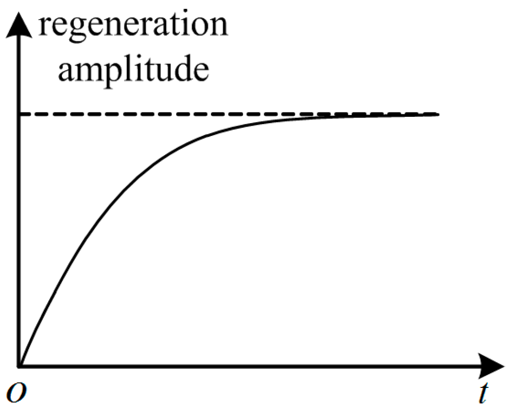
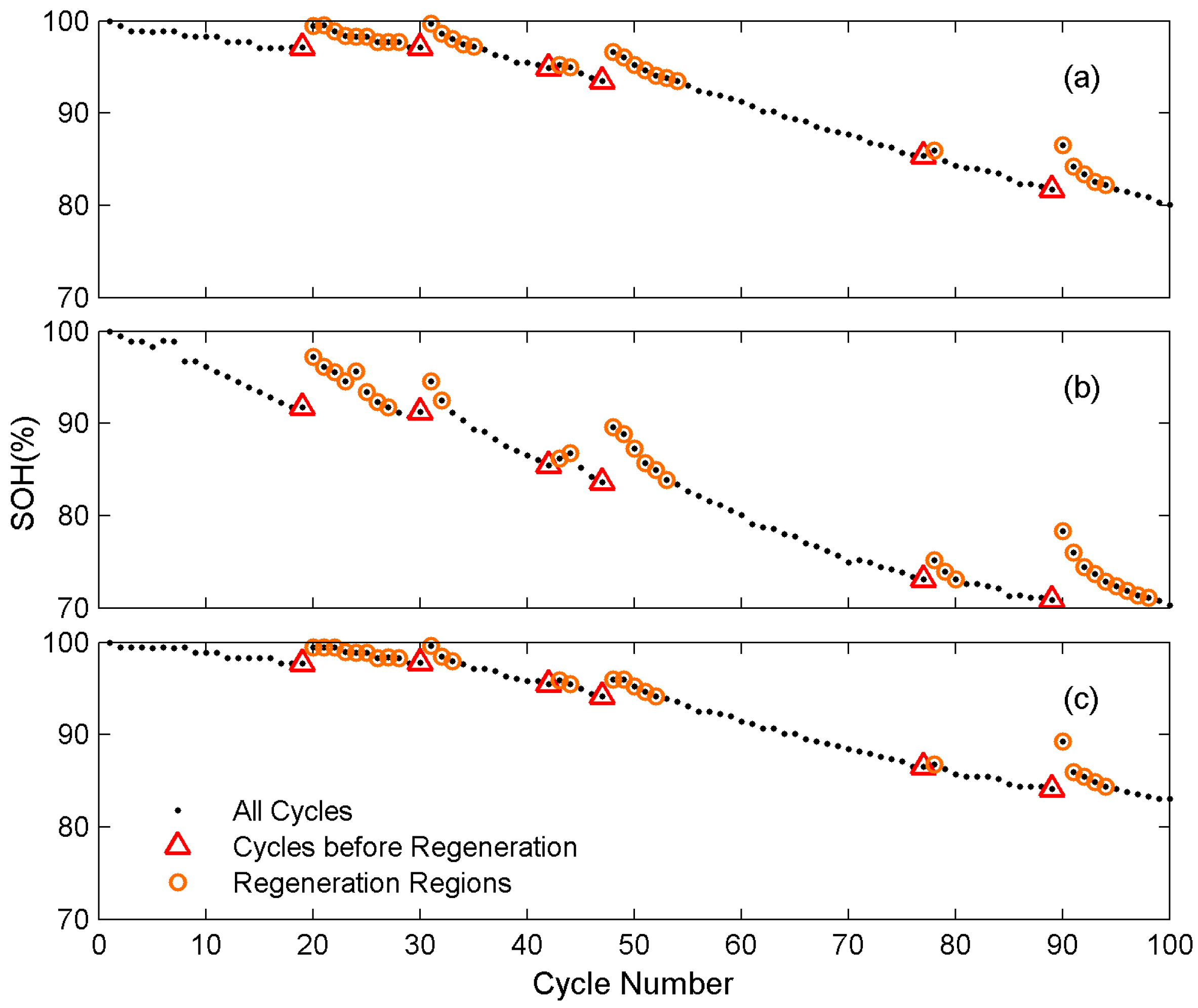
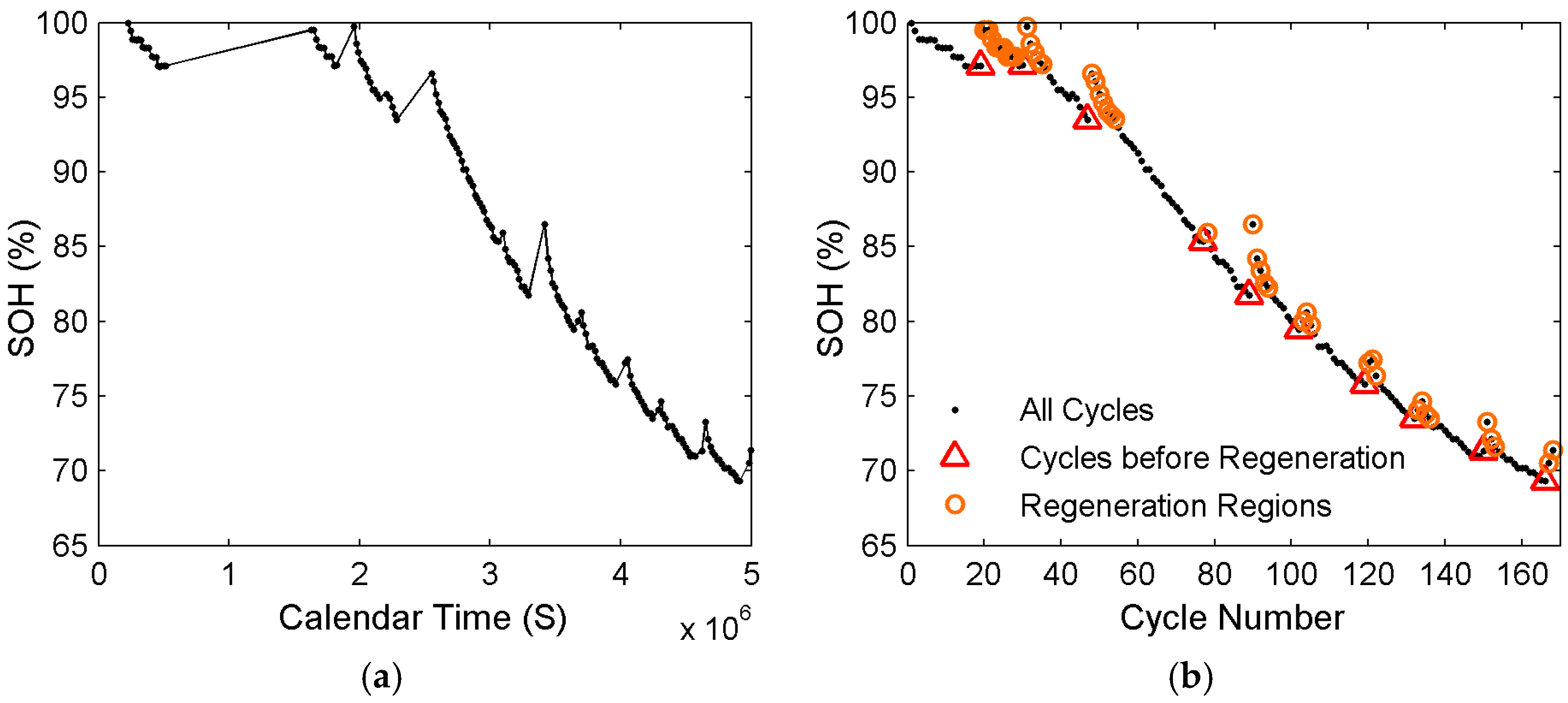
3.1. The Regeneration Phenomenon in Battery Degradation

In this paper, capacity is adopted to indicate the SOH of lithium-ion batteries, and it can be calculated by integrating current over time from full charge to full discharge. The relationship between SOH and capacity is described as:

$$\mathrm{SOH}=\frac{C_i}{C_0}\times 100\%$$

(21)

where C_i is the capacity value of cycle i and C₀ is the initial capacity value with no degradation.

Many articles have mentioned that capacity regeneration can improve the health state of the battery and slow down battery aging, and it has been confirmed by controlled experiments by Eddahech et al. [24]. However, the mechanism of capacity regeneration is still a much-debated topic. Agubra and Fergus [36] suggested that the loss or consumption of recyclable lithium ions due to the growth of the solid–electrolyte interface (SEI) layer is a main cause of the reduction in the reversible capacity of the lithium ion battery. During the rest time, the acidic impurities generated at the positive electrode can destroy the SEI layer at the negative and liberate lithium ions [37,38]. Eddahech et al. [39] pointed out that recovery phenomenon may be related to charge redistribution when there is no charge or discharge force acting on them. Baghdadi et al. [40] argued that a rearrangement of the lithium within the active material crystalline structure occurs thanks to solid diffusion during the battery rest. Thus, less disorder and more accessibility to lithium intercalation sites promotes the battery capacity, allowing more ampere-hours to be stored.

Figure 3 shows the battery SOH degradation data (Battery No. 5 from NASA Ames Prognostics Center of Excellence (PCoE) Center, Moffett Field, CA, USA). Figure 3a illustrates the curve of SOH and calendar time. The amplitude of SOH has an increase when the beginning time interval between two cycles is relatively long. It demonstrates that the regeneration phenomenon is obvious when the rest time is long enough. Figure 3b shows the relationship between SOH and cycle number. Moreover, we can see that after obvious regeneration appearance, SOH degradation rate at the next several cycles is much faster than before. Therefore, it is necessary to analyze the effects of regeneration and global degradation separately. We call the cycle with a significant capacity increase caused by a long rest time as “regeneration cycle” and the previous one cycle as “the cycle before regeneration”. Compared with the cycle before regeneration, the capacity values of the next several cycles increase. We call these cycles as “regeneration region”, the number of cycles in each regeneration region as “regeneration cycle number” and the cycle except regeneration regions as “global cycle”. These definitions will be directly used below and they are illustrated in Figure 3b.

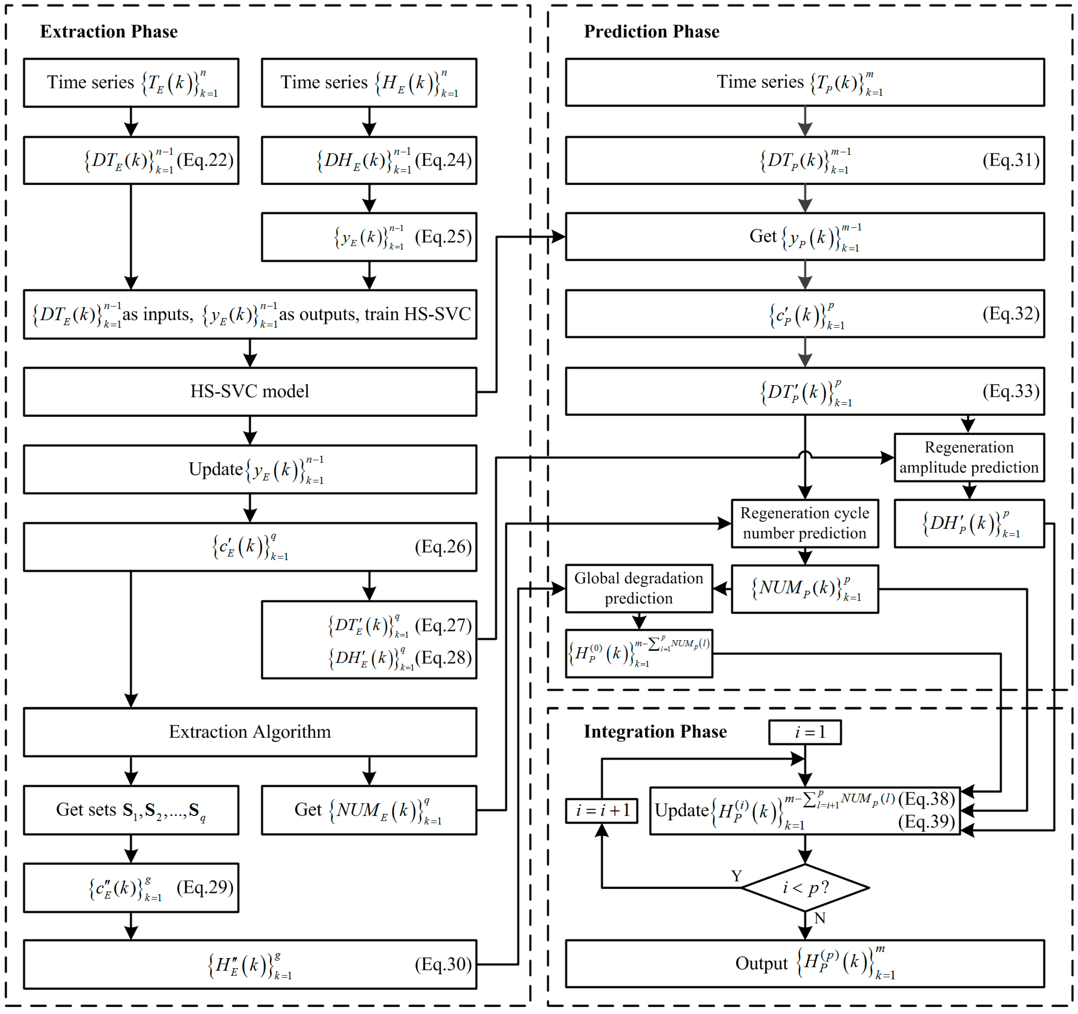
3.2. Rest Time-Based Prognostics Strategy

Our motivation is to decouple global degradation trend and regeneration, predict them respectively and then integrate them to get the overall prediction results. The proposed framework is outlined in Figure 4. This framework is composed of extraction phase, prediction phase and integration phase.

In extraction phase, it is assumed that the battery is fully charged in the initial state, and the cycle starts from discharge. ${\{T_E\left(k\right)\}}_{k=1}^n$ is a series of the calendar time of the beginning of each cycle. ${\{H_E\left(k\right)\}}_{k=1}^n$ is a time series of SOH from cycle 1 to cycle n, and it can be obtained by capacity monitoring during the usage of the battery. Also, cycle number series is denoted as ${\{c_E\left(k\right)\}}_{k=1}^n=\left\{1,2,...,n\right\}$.

${\{D{T}_E\left(k\right)\}}_{k=1}^{n-1}$ is the forward difference series of the beginning time of each cycle. $D{T}_E\left(k\right)$ is expressed as:

$$D{T}_E\left(k\right)=T_E\left(k+1\right)-T_E\left(k\right)$$

(22)

Moreover, $D{T}_E\left(k\right)$ can also be described by:

$$D{T}_E\left(k\right)=t_D\left(k\right)+t_C\left(k\right)+t_P\left(k\right)$$

(23)

where t_D(k) is the total discharge time of cycle k. t_C(k) is the total charge time of cycle k. t_P(k) is the total pause time (rest time) of cycle k. Although the battery may pause several times in a cycle, the lasting time of battery charge and discharge always has little change under certain working conditions. As a result, from Equation (23), the beginning time interval DT_E(k) is almost linear with the sum of pause time of cycle k. Moreover, compared with the rest time, the beginning time interval calculated by the recorded beginning time of each cycle is much easier to be obtained. Therefore, in this paper, the beginning time interval instead of the rest time is adopted as the input of this framework.

${\{D{H}_E\left(k\right)\}}_{k=1}^{n-1}$ is the forward difference series of SOH, where DH_E(k) is the SOH increment between cycle k and k + 1 and is shown as:

$$D{H}_E\left(k\right)=H_E\left(k+1\right)-H_E\left(k\right)$$

(24)

If the SOH of cycle (k + 1) is much better than that of cycle k, there may be significant regeneration, measurement errors, unexpected fluctuations and other factors during this period. ${\{y_E\left(k\right)\}}_{k=1}^{n-1}$ is to distinguish whether obvious SOH regeneration has appeared in each cycle.

$$y_E(k)=\{\begin{array}{cc}1,& D{H}_E\left(k\right)<Th\\ -1,& D{H}_E\left(k\right)\ge Th\end{array}$$

(25)

where $y_E\left(k\right)=-1$ means that the value of capacity has a large increase from cycle k to cycle (k + 1), while $y_E\left(k\right)=1$ means the opposite. Th is the given threshold to distinguish between the two states.

Generally, regeneration cycles account for a very small number of the total cycles, which makes the dataset $\left\{\left(D{T}_E\left(k\right),y_E\left(k\right)\right)|k=1,2,...,n-1\right\}$ unbalanced. Moreover, in the SOH degradation data, there is noise besides regeneration, and they are linearly non-separable. In this situation, some common methods, such as PLA, are not applicable. That is because PLA can only solve linearly separable problems. However, SVM-HS model can well balance the accuracy and generalization with the linearly non-separable samples. The hyperplane shift parameter $p$ can be determined according to the unbalanced degree of the two-class data. Significantly, in this case, $d=1$ and $\left[R^2/M^2\right]\ge 1$, so the VC dimension of SVM-HS equals to 2 and it is the same as that of PLA. This mean that the complexity of SVM-HS and that of PLA is the same.

Then, the trained SVM-HS model is used to update ${\{y_E\left(k\right)\}}_{k=1}^{n-1}$. This is to ensure that the capacity value increase is indeed caused by regeneration. Put the cycle before regeneration into set ${\mathbf{C}}_E^{\prime }$ which can be described by:

$${\mathbf{C}}_E^{\prime }=\left\{k|y_E\left(k\right)=-1,1\le k\le n-1\right\}$$

(26)

It is assumed that ${\mathbf{C}}_E^{\prime }$ contains $q$ elements. It means that obvious regeneration of the battery has appeared $q$ times. We sort the elements of ${\mathbf{C}}_E^{\prime }$ in ascending order and then get a new series ${\{c_E^{\prime }\left(k\right)\}}_{k=1}^q$. The time interval between the beginning of cycle $c_E^{\prime }\left(k\right)$ and cycle $\left(c_E^{\prime }\left(k\right)+1\right)$ is expressed as:

$$D{T}_E^{\prime }\left(k\right)=D{T}_E\left(c_E^{\prime }\left(k\right)\right)$$

(27)

The regeneration capacity amplitude from cycle $c_E^{\prime }\left(k\right)$ to cycle $\left(c_E^{\prime }\left(k\right)+1\right)$ is described by:

$$D{H}_E^{\prime }\left(k\right)=D{H}_E\left(c_E^{\prime }\left(k\right)\right)$$

(28)

The algorithm to extract regeneration region sets and regeneration cycle number series are as Algorithm 1.

Algorithm 1. Extraction of regeneration region sets and regeneration cycle number series.
1:	for $i=1$ to $q$ do
2:	set $j=1$
3:	while ($c_E^{\prime }\left(i\right)+j\le n$) and ($H\left(c_E^{\prime }\left(i\right)+j\right)-H\left(c_E^{\prime }\left(i\right)\right)\ge 0$) do
4:	put cycle number $c_E^{\prime }\left(i\right)+j$ into set $S_i$
5:	$j=j+1$
6:	end while
7:	end for
8:	for $i=1$ to $q-1$ do
9:	for $j=i+1$ to $q$ do
10:	$S_i=S_i-S_j$
11:	end for
12:	$NU{M}_E\left(i\right)=\left|S_i\right|$
13:	end for
14:	$NU{M}_E\left(q\right)=\left|S_q\right|$

All the cycle numbers of global degradation are denoted by set ${\mathbf{C}}_E^{\mathbf{″}}$, which can be expressed as:

$${\mathbf{C}}_E^{\mathbf{″}}={\mathbf{C}}_E-{\displaystyle \sum _{i=1}^q{S}_i}$$

(29)

We sort the g elements of ${\mathbf{C}}_E^{\mathbf{″}}$ into ascending order and get a new series ${\{c_E^{″}\left(k\right)\}}_{k=1}^g$. With series ${\{c_E^{″}\left(k\right)\}}_{k=1}^g$, the global degradation of SOH can be described by:

$$H_E^{″}\left(k\right)=H_E\left(c_E^{″}\left(k\right)\right)$$

(30)

In prediction phase, ${\{T_p\left(k\right)\}}_{k=1}^m$ consists of the beginning time of cycle (n + 1) to cycle (n + m). It is used for SOH prediction and can be acquired from the working plan or history information of used relevant batteries. Cycle number series is ${\left\{c_p\left(k\right)\right\}}_{k=1}^m=\left\{n+1,n+2,...,n+m\right\}$. ${\left\{D{T}_p\left(k\right)\right\}}_{k=1}^{m-1}$ is the forward difference series of the beginning time of each cycle, where $D{T}_p\left(k\right)$ is as:

$$D{T}_p\left(k\right)=\{\begin{array}{l}{T}_p\left(k+1\right)-T_p\left(k\right),k=1,2,...,m-1\\ T_p\left(k+1\right)-T_E\left(n\right),k=0\end{array}$$

(31)

Using series ${\{D{T}_p\left(k\right)\}}_{k=0}^{m-1}$ as the input, the trained SVM-HS model is adopted to predict the value of ${\{y_p\left(k\right)\}}_{k=0}^{n-1}$. Put the cycles before regeneration into set ${\mathbf{C}}_p^{\mathbf{\prime }}$ which can be described by:

$${\mathbf{C}}_p^{\mathbf{\prime }}=\left\{k|y_p\left(k\right)=-1,0\le k\le m-1\right\}$$

(32)

With the assumption that obvious regeneration phenomena have happened p times, there are p elements in ${\mathbf{C}}_p^{\mathbf{\prime }}$. Sort them into ascending order and then get the series ${\{c_p^{\prime }\left(k\right)\}}_{k=1}^p$. Long time intervals that lead to obvious regeneration compose the series ${\{D{T}_p^{\prime }\left(k\right)\}}_{k=1}^p$, where $D{T}_p^{\prime }\left(k\right)$ is as:

$$D{T}_p^{\prime }\left(k\right)=D{T}_p\left(c_p^{\prime }\left(k\right)\right)$$

(33)

Based on the regeneration amplitude prediction algorithm, the series ${\{D{H}_p^{\prime }\left(k\right)\}}_{k=1}^p$ can be predicted. Also, based on the regeneration cycle number prediction algorithm, the series ${\{NU{M}_p\left(k\right)\}}_{k=1}^p$ can be predicted. Taking global SOH degradation series ${\{H_E^{″}\left(k\right)\}}_{k=1}^g$ as the training samples, the $m-{\displaystyle {\sum }_{l=1}^{p}NU{M}_p\left(l\right)}$ steps’ SOH prediction values of global degradation can be obtained and written as ${\{H_p^{(0)}\left(k\right)\}}_{k=1}^{m-{\displaystyle {\sum }_{l=1}^{p}NU{M}_p\left(l\right)}}$.

The capacity regeneration phenomenon is strongly related to the rest time but it is not affected by aging, because the phenomenon is reproduced in the same way even when the battery becomes aged [24]. The relationship between rest time and the amplitude of capacity regeneration is a nonlinear correlation. The battery can be at rest for a very long time, but capacity regeneration amplitude is limited. Therefore, as shown in Figure 5, we assume that the increase rate of capacity regeneration amplitude declines as the rest time increases.

The mapping function adopted in this article is a hyperbolic tangent function which is widely used in machine learning. It is described as:

$$\mathsf{\phi }(t)=\frac{e^{c\cdot t}-e^{-c\cdot t}}{e^{c\cdot t}+e^{-c\cdot t}}$$

(34)

where $c$ is a length-scale parameter. The relationship between regeneration amplitude and $D{T}^{\prime }\left(k\right)$ can be expressed by:

$$D{H}_p^{\prime }\left(k\right)=s\cdot \mathsf{\phi }\left(D{T}_p^{\prime }\left(k\right)\right)$$

(35)

Therefore, the elements of ${\{D{H}_p^{\prime }\left(k\right)\}}_{k=1}^p$ can be predicted by:

$$D{H}_p^{\prime }\left(k\right)=\mathsf{\phi }\left(D{T}_p^{\prime }\left(k\right)\right)\cdot \left(\frac{1}{q}{\displaystyle \sum _{i=1}^q\frac{D{H}_E^{\prime }\left(i\right)}{\mathsf{\phi }\left(D{T}_E^{\prime }\left(i\right)\right)}}\right)$$

(36)

Similarly, we assume that the increase rate of regeneration cycle number declines with the increase of rest time and take hyperbolic tangent function as the mapping function. Thus, the regeneration cycle number series ${\{NU{M}_p\left(k\right)\}}_{k=1}^p$ can be predicted by:

$$NU{M}_p\left(k\right)=\left[\mathsf{\phi }\left(D{T}_p^{\prime }\left(k\right)\right)\cdot \left(\frac{1}{q}{\displaystyle \sum _{i=1}^q\frac{NU{M}_E\left(i\right)}{\mathsf{\phi }\left(D{T}_E^{\prime }\left(i\right)\right)}}\right)+\frac{1}{2}\right]$$

(37)

In this paper, Gaussian process model recommended in Section 2.2 is used in global degradation prediction.

In the integration phase, the predicted SOH values of each regeneration region are added into the global regeneration series. Then, the SOH prediction values of all cycles are obtained. The SOH series of the ith regeneration region is as ${\{R{H}_p^{\left(i\right)}\left(k\right)\}}_{k=1}^{NU{M}_p\left(i\right)}$. Based on the assumption that SOH linearly degrades in the regeneration regions, the value of element $R{H}_p^{\left(i\right)}\left(k\right)$ can be calculated by:

$$R{H}_p^{\left(i\right)}\left(k\right)=H_p^{\left(i-1\right)}\left(c_p^{\prime }\left(i\right)-n\right)+\frac{D{H}_p^{\prime }\left(i\right)}{NU{M}_p(i)}\cdot \left(NU{M}_p\left(i\right)-k+1\right)$$

(38)

Series ${\{H_p^{\left(i\right)}\left(k\right)\}}_{k=1}^{m-{\displaystyle {\sum }_{l=i+1}^{p}NU{M}_p\left(l\right)}}$ is updated by:

$$\begin{array}{ll}{\left\{H_p^{\left(i\right)}\left(k\right)\right\}}_{k=1}^{m-{\displaystyle {\sum }_{l=i+1}^{p}NU{M}_p\left(l\right)}}=& \{H_p^{\left(i-1\right)}\left(1\right),\cdot \cdot \cdot ,H_p^{\left(i-1\right)}\left(c_p^{\prime }\left(i\right)-n\right),R{H}_p^{\left(i\right)}\left(1\right),\cdot \cdot \cdot ,R{H}_p^{\left(i\right)}\left(NU{M}_p\left(i\right)\right),\\ & H_p^{\left(i-1\right)}\left(c_p^{\prime }\left(i\right)-n+1\right),\cdot \cdot \cdot ,H_p^{\left(i-1\right)}\left(m-{\displaystyle {\sum }_{l=i+1}^{p}NU{M}_p\left(l\right)}\right)\}\end{array}$$

(39)

For different sizes and chemistries of lithium-ion batteries, the capacity regeneration phenomenon may or may not appear. If it appears, the proposed framework can be used for decoupling the global degradation and local regeneration; and if capacity regeneration phenomenon doesn’t appear, the value of discriminate function (Equation (25)) always equals to 1 and the proposed framework only contains prediction method of global degradation. In other words, ${\{H_p^{(p)}\left(k\right)\}}_{k=1}^m={\{H_p^{(0)}\left(k\right)\}}_{k=1}^m$. Therefore, the proposed framework is applicable for different batteries with or without the capacity regeneration phenomenon.

4. Experimental Section

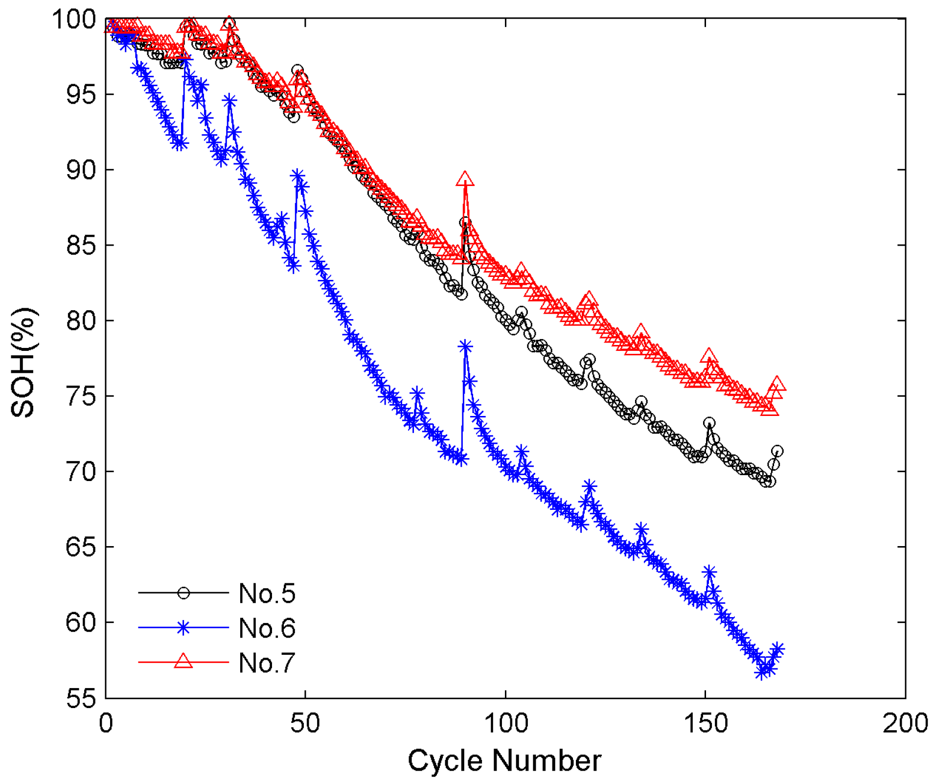
4.1. Battery Data Set

The lithium-ion battery capacity degradation data adopted to conduct the experiments of SOH prediction are obtained from the data repository of the NASA Ames PCoE [41]. A set of commercial 18,650 lithium-ion batteries were run at room temperature through three operational profiles (charge, discharge, and impedance). Charging was carried out at a constant level of 1.5 A until the battery voltage is up to 4.2 V and then it was continued with the voltage of 4.2 V until the charge current fell to 20 mA. Discharge was carried out in a constant mode at 2 A until the battery voltage dropped to 2.7, 2.5, and 2.2 V for batteries Nos. 5, 6, and 7, respectively. Impedance was measured by an electrochemical impedance spectroscopy (EIS) with frequency from 0.1 to 5 kHz. Repeated charge and discharge of the batteries resulted in their accelerated aging. The experiments were stopped when the batteries reached end-of-life criteria, a 30% fade in rated capacity (from 2 to 1.4 Ah).

Based on Equation (21), SOH can be easily derived from the experimental capacity data. Figure 6 shows the evolution of SOH for batteries Nos. 5, 6, and 7. The total charge/discharge cycles are all 168 for these three batteries. It can be seen from Figure 5 that the SOH time series presents clear regeneration phenomena, and the SOH degradation rate of the cycles in the regeneration region is much faster. It is, therefore, important to extract these cycles for prediction model construction. The capacity degradation data from cycle 1 to cycle 100 are selected as the training samples to predict the future SOH values, while the data from cycle 101 to cycle 168 are used for prediction performance evaluation of this improved framework.

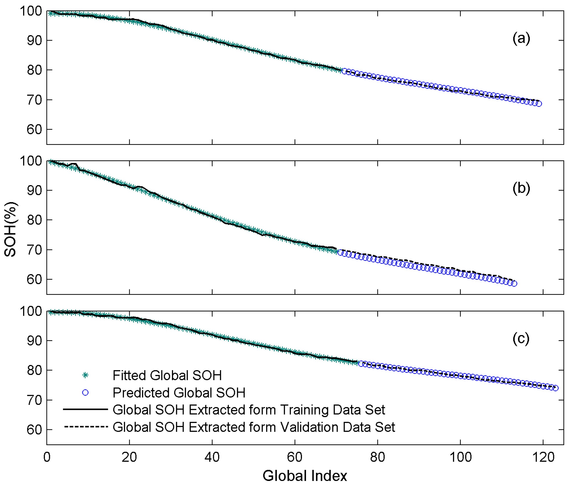
4.2. Prediction and Comparison

The SOH values and the beginning time of the first 100 cycles are adopted as the inputs of the method given in Section 3 to extract the regeneration information. In this paper, the threshold is set at 0.2% (Th = 0.2%) and the hyperplane shift parameter is set at −0.5 (p = −0.5).

The extraction results of regeneration information are illustrated in Figure 7. From the figure, we can see that all the cycles with a remarkable increase of SOH value are extracted from the 100 training samples. It indicates that for these three sets of degradation data, regeneration is the main factor of capacity fluctuations. Moreover, all the extracted cycles before regeneration of the three batteries are the same. This is because, in the experiments, the three batteries have the same beginning time of every cycle. However, for these three batteries, regeneration amplitude and regeneration cycle number of each regeneration region are different. This is because of individual differences and their different working conditions.

Using the intervals of the beginning time of two adjacent cycles which can be known from battery working plan as the input, the cycle before regeneration series ${\left\{c_p^{\prime }\left(k\right)\right\}}_{k=1}^p$ can be predicted with the trained SVM-HS model obtained from the extraction phrase. Although the corresponding series ${\left\{c_p^{\prime }\left(k\right)\right\}}_{k=1}^p$ and ${\left\{D{T}_p^{\prime }\left(k\right)\right\}}_{k=1}^p$ are determined by different SVM-HS models, all the predicted cycles before regeneration of batteries Nos. 5, 6, and 7 are the same. This is because the rest time of the three batteries is similar. The prediction results of ${\left\{c_p^{\prime }\left(k\right)\right\}}_{k=1}^p$ and ${\left\{D{T}_p^{\prime }\left(k\right)\right\}}_{k=1}^p$ are shown in

Table 1. Cycle before regeneration and corresponding beginning time intervals.

k	1	2	3	4	5
$c_p^{\prime }\left(k\right)$	102	119	132	149	166
$D{T}_p^{\prime }\left(k\right)$	10.33	20.97	12.12	15.22	19.53

.

The regeneration cycle number of batteries Nos. 5, 6, and 7 is predicted based on Equation (37). The results are shown in

Table 2. Regeneration cycle number.

k	1	2	3	4	5
No. 5	3	5	4	4	5
No. 6	4	5	4	5	5
No. 7	3	4	3	4	4

.

The regeneration amplitude of batteries Nos. 5, 6, and 7 predicted by Equation (36) is shown in

Table 3. Regeneration amplitude (%).

k	1	2	3	4	5
No. 5	1.07	1.85	1.23	1.48	1.77
No. 6	2.15	3.73	2.47	2.98	3.56
No. 7	0.87	1.51	1.00	1.21	1.44

.

The curves of global SOH degradation of three batteries are illustrated in Figure 8. Compared with the curves in Figure 6, they are smooth and have fewer fluctuations. GP model is used to predict the global degradation of SOH values of the batteries Nos. 5, 6, and 7, and the initial hyper-parameters $\mathsf{\Theta }=\left[l,{\mathsf{\sigma }}_f,{\mathsf{\sigma }}_n\right]$ are set by experience, as l = g, ${\mathsf{\sigma }}_f=\max \left(D{H}_t^{\prime }(k_1)\right)-\min \left(D{H}_t^{\prime }\left(k_2\right)\right)$ $\left(k_1=1,2,...,t;k_2=1,2,...,t\right)$, ${\mathsf{\sigma }}_n=1.5\max \left(\left|D{H}_t^{\prime }(k)-D{H}_t^{\prime }\left(k+1\right)\right|\right)$ $\left(k=1,2,...,t-1\right)$. The particle swarm optimization algorithm is used to determine the hyper-parameters of GP model for the three batteries and the final values are ${\mathsf{\Theta }}_{No.5}=\left[70.95,0.1958,0.0081\right]$, ${\mathsf{\Theta }}_{No.6}=\left[68.81,0.2977,0.0335\right]$ and ${\mathsf{\Theta }}_{No.7}=\left[75.25,0.1702,0.0090\right]$. The detailed implementation of particle swarm optimization algorithm could refer to our previous work [28]. The SOH prediction results of global degradation are shown in Figure 8. It can be seen intuitively that the predicted global SOH results of the three batteries are close to the real validation data. That is because after decoupling from regeneration, the global degradation trend is smooth and easier to be accurately predicted.

After integrating the prediction results of regeneration and global degradation, the final prediction results are obtained and shown in Figure 9. It is clear that based on this framework, for the three batteries, the predicted regeneration cycles are exactly the real regeneration cycles. Also, regeneration values of cycles in the regeneration regions are well predicted, which makes the prediction error around the regeneration cycles small.

Two criteria, mean absolute percentage error (MAPE) and root mean square error (RMSE), are adopted to evaluate the prediction performance of different methods.

$$RMSE=\sqrt{\frac{1}{N}{\displaystyle {\sum }_{i=1}^N{\left(y_i-{\widehat{y}}_i\right)}^2}}$$

(40)

$$MAPE=\frac{1}{N}{\displaystyle \sum _{i=1}^N\left|\frac{y_i-{\widehat{y}}_i}{y_i}\right|}\times 100\%$$

(41)

Table 4. Comparison of different prognostic methods for batteries Nos. 5, 6, and 7. RTPF: rest time-based prognostic framework.

Battery No.	5		6		7
Error Criteria	MAPE (%)	RMSE	MAPE (%)	RMSE	MAPE (%)	RMSE
LGPFR 1	23.0	1.71	10.30	6.90	1.90	1.59
QGPFR 1	1.90	1.50	7.70	5.12	5.40	5.52
C-LGPFR 1	1.60	1.36	10.20	6.86	1.70	1.73
C-QGPFR 1	2.10	1.80	29.0	20.44	2.60	2.69
SMK-GPR 2	1.65	1.38	10.60	7.08	1.91	1.88
P-MGPR 2	1.55	1.36	2.96	2.12	1.09	1.14
SE-MGPR 2	1.38	1.20	2.93	2.11	1.02	1.07
IPSO-SVR 3	0.82	0.75	2.28	1.66	1.02	0.97
RTPF	0.76	0.68	1.25	0.93	0.43	0.44

¹ Results of these methods are obtained from reference [15]; ² Results of these methods are obtained from reference [25]; ³ Results of these methods are obtained from reference [28].

presents the comparison results of the prediction performance of different methods for batteries Nos. 5, 6 and 7. The prediction errors of published methods are obtained from reference [15,25,28]. It is clear that the proposed RTPF has much better prediction performance than the eight published methods. More specifically, the smallest prediction MAPE on batteries Nos. 5, 6 and 7 among the eight published models are 0.82%, 2.28% and 1.02% respectively, while the counterparts of this proposed framework are 0.76%, 1.25% and 0.43% respectively. Similarly, compared to these published methods, the prognostic RMSE of RTPF on three batteries are also the smallest. There are two possible reasons. One reason is that this framework can accurately predict the regeneration cycles, and another reason is that global SOH degradation trend without the effects of regeneration becomes smooth and easier to predict.

Moreover, different types of discharge/charge profiles may lead to the different degrees of capacity regeneration. If there are regeneration phenomena during battery degradation, this framework can be employed to decouple global degradation trend and regeneration. In this article, the prediction methods of global degradation, regeneration amplitude and regeneration cycle number are all data-driven approaches which realize prediction (extrapolation) by learning from training samples. Therefore, for different capacity regeneration phenomena, the parameters of these three prediction methods will be adopted from corresponding training samples to suit various degradation trends. Therefore, for different discharge/charge profiles, the parameters of prediction models (global degradation prediction model, regeneration cycle number prediction model, and regeneration amplitude prediction model) would be changed, while the structure of this framework would not be changed.

5. Conclusions

To obtain more accurate long-term prediction results of battery SOH with capacity regeneration phenomenon, we have proposed a RTPF. It consists of extraction phase, prediction phase and integration phase. Based on this framework, regeneration phenomenon and global degradation are decoupled. The two parts are predicted separately and finally integrated together to obtain the overall SOH degradation results. SVM-HS model is proposed to classify the unbalanced dataset of beginning time intervals of two adjacent cycles. Moreover, GP model is used to predict the global degradation trend of battery SOH, and nonlinear models are utilized to predict the regeneration amplitude and the cycle number of each regeneration region, respectively.

Case studies are carried out to evaluate the performance of the proposed framework. The results show that: (1) in extraction phase, SVM-HS model can extract the beginning time intervals of two adjacent cycles that cause obvious capacity regeneration; in prediction phase, it can successfully predict all the cycles before regeneration; (2) even around the regeneration cycles, this framework also has a high prediction accuracy; and (3) using the previous capacity data of the current battery, compared with the published methods, this model can achieve more accurate SOH prediction results.

References

1. Abada, S.; Marlair, G.; Lecocq, A.; Petit, M.; Sauvant-Moynot, V.; Huet, F. Safety focused modeling of lithium-ion batteries: A review. J. Power Sources 2016, 306, 178–192. [Google Scholar] [CrossRef]
2. Xing, Y.J.; Ma, E.W.M.; Tsui, K.L.; Pecht, M. An ensemble model for predicting the remaining useful performance of lithium-ion batteries. Microelectron. Reliab. 2013, 53, 811–820. [Google Scholar] [CrossRef]
3. Liu, J.; Wang, W.; Golnaraghi, F. An enhanced diagnostic scheme for bearing condition monitoring. IEEE Trans. Instrum. Meas. 2010, 59, 309–321. [Google Scholar]
4. Williard, N.; He, W.; Hendricks, C.; Pecht, M. Lessons learned from the 787 dreamliner issue on lithium-ion battery reliability. Energies 2013, 6, 4682–4695. [Google Scholar] [CrossRef]
5. Wang, S.; Zhao, L.; Su, X.; Ma, P. Prognostics of lithium-ion batteries based on battery performance analysis and flexible support vector regression. Energies 2014, 7, 6492–6508. [Google Scholar] [CrossRef]
6. Zheng, X.J.; Fang, H.J. An integrated unscented kalman filter and relevance vector regression approach for lithium-ion battery remaining useful life and short-term capacity prediction. Reliab. Eng. Syst. Saf. 2015, 144, 74–82. [Google Scholar] [CrossRef]
7. Rezvanizaniani, S.M.; Liu, Z.C.; Chen, Y.; Lee, J. Review and recent advances in battery health monitoring and prognostics technologies for electric vehicle (EV) safety and mobility. J. Power Sources 2014, 256, 110–124. [Google Scholar] [CrossRef]
8. An, D.; Kim, N.H.; Choi, J.H. Practical options for selecting data-driven or physics-based prognostics algorithms with reviews. Reliab. Eng. Syst. Saf. 2015, 133, 223–236. [Google Scholar] [CrossRef]
9. Hendricks, C.; Williard, N.; Mathew, S.; Pecht, M. A failure modes, mechanisms, and effects analysis (FMMEA) of lithium-ion batteries. J. Power Sources 2015, 297, 113–120. [Google Scholar] [CrossRef]
10. Li, Y.; Yang, J.; Song, J. Microscale characterization of coupled degradation mechanism of graded materials in lithium batteries of electric vehicles. Renew. Sustain. Energy Rev. 2015, 50, 1445–1461. [Google Scholar] [CrossRef]
11. Berecibar, M.; Gandiaga, I.; Villarreal, I.; Omar, N.; Van Mierlo, J.; Van den Bossche, P. Critical review of state of health estimation methods of li-ion batteries for real applications. Renew. Sustain. Energy Rev. 2016, 56, 572–587. [Google Scholar] [CrossRef]
12. Long, B.; Xian, W.M.; Jiang, L.; Liu, Z. An improved autoregressive model by particle swarm optimization for prognostics of lithium-ion batteries. Microelectron. Reliab. 2013, 53, 821–831. [Google Scholar] [CrossRef]
13. Saha, B.; Goebel, K.; Poll, S.; Christophersen, J. Prognostics methods for battery health monitoring using a bayesian framework. IEEE Trans. Instrum. Meas. 2009, 58, 291–296. [Google Scholar] [CrossRef]
14. Miao, Q.; Xie, L.; Cui, H.J.; Liang, W.; Pecht, M. Remaining useful life prediction of lithium-ion battery with unscented particle filter technique. Microelectron. Reliab. 2013, 53, 805–810. [Google Scholar] [CrossRef]
15. Liu, D.T.; Pang, J.Y.; Zhou, J.B.; Peng, Y.; Pecht, M. Prognostics for state of health estimation of lithium-ion batteries based on combination gaussian process functional regression. Microelectron. Reliab. 2013, 53, 832–839. [Google Scholar] [CrossRef]
16. Tang, S.; Yu, C.; Wang, X.; Guo, X.; Si, X. Remaining useful life prediction of lithium-ion batteries based on the wiener process with measurement error. Energies 2014, 7, 520–547. [Google Scholar] [CrossRef]
17. Widodo, A.; Shim, M.C.; Caesarendra, W.; Yang, B.S. Intelligent prognostics for battery health monitoring based on sample entropy. Expert Syst. Appl. 2011, 38, 11763–11769. [Google Scholar] [CrossRef]
18. Guo, J.; Li, Z.J.; Pecht, M. A Bayesian approach for Li-ion battery capacity fade modeling and cycles to failure prognostics. J. Power Sources 2015, 281, 173–184. [Google Scholar] [CrossRef]
19. Andre, D.; Appel, C.; Soczka-Guth, T.; Sauer, D.U. Advanced mathematical methods of SOC and SOH estimation for lithium-ion batteries. J. Power Sources 2013, 224, 20–27. [Google Scholar] [CrossRef]
20. Liu, D.T.; Wang, H.; Peng, Y.; Xie, W.; Liao, H.T. Satellite lithium-ion battery remaining cycle life prediction with novel indirect health indicator extraction. Energies 2013, 6, 3654–3668. [Google Scholar] [CrossRef]
21. Chen, C.C.; Zhang, B.; Vachtsevanos, G. Prediction of machine health condition using neuro-fuzzy and bayesian algorithms. IEEE Trans. Instrum. Meas. 2012, 61, 297–306. [Google Scholar] [CrossRef]
22. Jin, G.; Matthews, D.E.; Zhou, Z. A Bayesian framework for on-line degradation assessment and residual life prediction of secondary batteries in spacecraft. Reliab. Eng. Syst. Saf. 2013, 113, 7–20. [Google Scholar] [CrossRef]
23. Saha, B.; Goebel, K. Modeling Li-ion battery capacity depletion in a particle filtering framework. In Proceedings of the Annual Conference of the Prognostics and Health Management Society, San Diego, CA, USA, 27 September–1 October 2009; pp. 1–10.
24. Eddahech, A.; Briat, O.; Vinassa, J.-M. Lithium-ion battery performance improvement based on capacity recovery exploitation. Electrochim. Acta 2013, 114, 750–757. [Google Scholar] [CrossRef]
25. He, Y.J.; Shen, J.N.; Shen, J.F.; Ma, Z.F. State of health estimation of lithium-ion batteries: A multiscale gaussian process regression modeling approach. AIChE J. 2015, 61, 1589–1600. [Google Scholar] [CrossRef]
26. Olivares, B.E.; Munoz, M.A.C.; Orchard, M.E.; Silva, J.F. Particle-filtering-based prognosis framework for energy storage devices with a statistical characterization of state-of-health regeneration phenomena. IEEE Trans. Instrum. Meas. 2013, 62, 364–376. [Google Scholar] [CrossRef]
27. Orchard, M.E.; Lacalle, M.S.; Olivares, B.E.; Silva, J.F.; Palma-Behnke, R.; Estevez, P.A.; Severino, B.; Calderon-Munoz, W.; Cortes-Carmona, M. Information-theoretic measures and sequential monte carlo methods for detection of regeneration phenomena in the degradation of lithium-ion battery cells. IEEE Trans. Reliab. 2015, 64, 701–709. [Google Scholar] [CrossRef]
28. Qin, T.C.; Zeng, S.K.; Guo, J.B. Robust prognostics for state of health estimation of lithium-ion batteries based on an improved PSO-SVR model. Microelectron. Reliab. 2015, 55, 1280–1284. [Google Scholar] [CrossRef]
29. Li, F.; Xu, J.P. A new prognostics method for state of health estimation of lithium-ion batteries based on a mixture of gaussian process models and particle filter. Microelectron. Reliab. 2015, 55, 1035–1045. [Google Scholar] [CrossRef]
30. He, W.; Williard, N.; Osterman, M.; Pecht, M. Prognostics of lithium-ion batteries based on dempster-shafer theory and the bayesian monte carlo method. J. Power Sources 2011, 196, 10314–10321. [Google Scholar] [CrossRef]
31. Schölkopf, B.; Smola, A.J. Learning with Kernels: Support Vector Machines, Regularization, Optimization, and Beyond; MIT Press: Cambridge, MA, USA, 2002. [Google Scholar]
32. Abu-Mostafa, Y.S.; Magdon-Ismail, M.; Lin, H.T. Learning from Data; AMLBook: Singapore, 2012. [Google Scholar]
33. Vapnik, V.N. Statistical Learning Theory; John Wiley & Sons: Hoboken, NJ, USA, 1998. [Google Scholar]
34. Brahim-Belhouari, S.; Bermak, A. Gaussian process for nonstationary time series prediction. Comput. Stat. Data Anal. 2004, 47, 705–712. [Google Scholar] [CrossRef]
35. Murphy, K.P. Machine Learning: A Probabilistic Perspective; MIT Press: Cambridge, MA, USA, 2012. [Google Scholar]
36. Agubra, V.; Fergus, J. Lithium ion battery anode aging mechanisms. Materials 2013, 6, 1310–1325. [Google Scholar] [CrossRef]
37. Wang, E.; Ofer, D.; Bowden, W.; Iltchev, N.; Moses, R.; Brandt, K. Stability of lithium ion spinel cells III. Improved life of charged cells. J. Electrochem. Soc. 2000, 147, 4023–4028. [Google Scholar] [CrossRef]
38. Spotnitz, R. Simulation of capacity fade in lithium-ion batteries. J. Power Sources 2003, 113, 72–80. [Google Scholar] [CrossRef]
39. Eddahech, A.; Briat, O.; Bertrand, N.; Delétage, J.-Y.; Vinassa, J.-M. Behavior and state-of-health monitoring of Li-ion batteries using impedance spectroscopy and recurrent neural networks. Int. J. Electr. Power Energy Syst. 2012, 42, 487–494. [Google Scholar] [CrossRef]
40. Baghdadi, I.; Briat, O.; Gyan, P.; Vinassa, J.M. State of health assessment for lithium batteries based on voltage-time relaxation measure. Electrochim. Acta 2016, 194, 461–472. [Google Scholar] [CrossRef]
41. Saha, B.; Goebel, K. Battery Data Set; National Aeronautics and Space Adminstration (NASA) Ames Prognostics Data Repository: Moffett Field, CA, USA, 2007.
Figure 1. The effects of noise of majority class: (a) without noise; and (b) with noise.
Energies 09 00896 g001
Figure 2. Hyperplane shifted with data points: (a) two classes are linearly separable; and (b) two classes are not linearly separable.
Energies 09 00896 g002
Figure 3. The experimental degradation data: (a) with calendar time; and (b) with cycle number.
Energies 09 00896 g003
Figure 4. Framework of rest time-based prognostic strategy.
Energies 09 00896 g004
Figure 5. The assumed relationship between rest time and regeneration amplitude.
Energies 09 00896 g005
Figure 6. State of Health (SOH) values of batteries Nos. 5, 6 and 7.
Energies 09 00896 g006
Figure 7. The extraction of regeneration influence: (a) battery No. 5; (b) battery No. 6; and (c) battery No. 7.
Energies 09 00896 g007
Figure 8. Prediction results of global degradation: (a) battery No. 5; (b) battery No. 6; and (c) battery No. 7.
Energies 09 00896 g008
Figure 9. Overall prediction results of SOH: (a) battery No. 5; (b) battery No. 6; and (c) battery No. 7.
Energies 09 00896 g009