Article

Numerical Simulations of the Effects of a Tidal Turbine Array on Near-Bed Velocity and Local Bed Shear Stress

by
Philip A. Gillibrand
1,*,
Roy A. Walters
2 and
Jason McIlvenny
1
1
Environmental Research Institute, North Highland College, University of the Highlands and Islands, Thurso, Caithness KW14 8YD, UK
2
Ocean-River Hydrodynamics, Victoria, BC V8Y 3H7, Canada
*
Author to whom correspondence should be addressed.
Energies 2016, 9(10), 852; https://doi.org/10.3390/en9100852
Submission received: 14 August 2016 / Revised: 22 September 2016 / Accepted: 7 October 2016 / Published: 21 October 2016
(This article belongs to the Special Issue Numerical Modelling of Wave and Tidal Energy)

Abstract

:
We apply a three-dimensional hydrodynamic model to consider the potential effects of energy extraction by an array of tidal turbines on the ambient near-bed velocity field and local bed shear stress in a coastal channel with strong tidal currents. Local bed shear stress plays a key role in local sediment dynamics. The model solves the Reynold-averaged Navier-Stokes (RANS) equations on an unstructured mesh using mixed finite element and finite volume techniques. Tidal turbines are represented through an additional form drag in the momentum balance equation, with the thrust imparted and power generated by the turbines being velocity dependent with appropriate cut-in and cut-out velocities. Arrays of 1, 4 and 57 tidal turbines, each of 1.5 MW capacity, were simulated. Effects due to a single turbine and an array of four turbines were negligible. The main effect of the array of 57 turbines was to cause a shift in position of the jet through the tidal channel, as the flow was diverted around the tidal array. The net effect of this shift was to increase near-bed velocities and bed shear stress along the northern perimeter of the array by up to 0.8 m·s−1 and 5 Pa respectively. Within the array and directly downstream, near-bed velocities and bed shear stress were reduced by similar amounts. Changes of this magnitude have the potential to modify the known sand and shell banks in the region. Continued monitoring of the sediment distributions in the region will provide a valuable dataset on the impacts of tidal energy extraction on local sediment dynamics. Finally, the mean power generated per turbine is shown to decrease as the turbine array increased in size.

1. Introduction

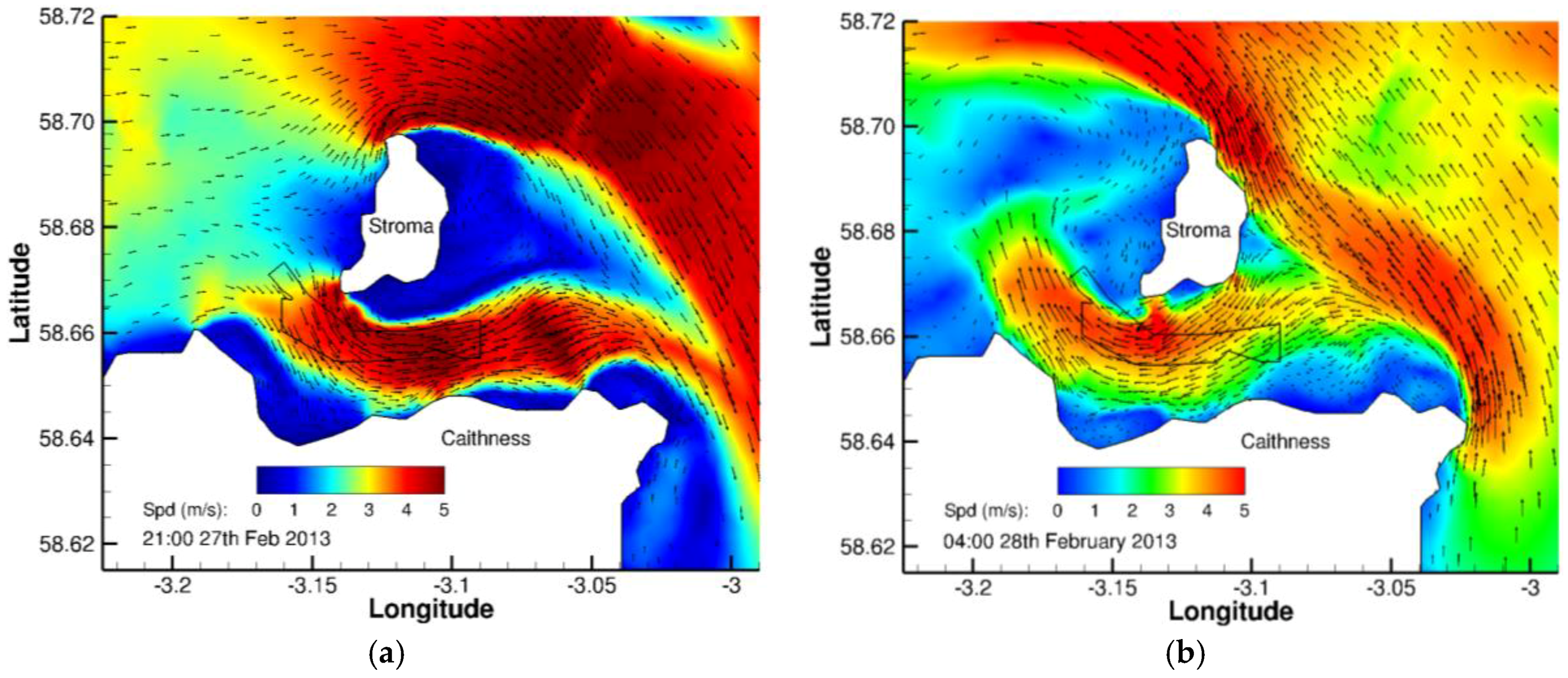
Over the past decade, the strong tidal flows in a number of regions around the world have been a focus of attention for tidal energy developers, with sites identified and leases granted for tidal energy extraction using tidal turbines. One of the primary areas of interest has been the Pentland Firth in the north of Scotland, which connects the North Sea and the North Atlantic and through which tidal current speeds regularly reach 5 m·s−1. The tidal energy potential for the whole Firth has been estimated to be in the range of 1–18 GW [1], though Adcock et al. [2] suggest that a more realistic figure for the maximum available power is 1.9 GW. At the time of writing, the Meygen tidal turbine array, planned for the Inner Sound channel of the Firth, is among the first commercial tidal energy arrays to be installed anywhere in the world. Tidal current speeds in the Inner Sound have been recorded at up to 6 m·s−1 during flood spring tides, offering an energy resource of up to 398 MW to the Meygen project [3].
Consent to deploy tidal turbines is generally subject to environmental impact assessment, with a requirement to demonstrate environmental effects within acceptable limits. Currently, these assessments typically focus on collision risk for marine mammals and seabirds, which present the highest impact risks. However, other, more subtle, environmental impacts arising from the deployment of large numbers of tidal turbines can be envisaged. These have been outlined by a number of authors, with the focus being mainly on ecological and socio-economic impacts (e.g., [4,5]).
One of the potential impacts of tidal energy is on sediment transport and the effect of energy extraction on the movement of sediment through these energetic channels. An early study by Neill et al. [6] demonstrated that installations of tidal energy convertors in the Bristol Channel (south-west UK) could influence large scale sediment dynamics and bed level changes. In a subsequent study, Neill et al. [7] found that tidal turbines could also impact sand bank formation and evolution near headlands. In the Pentland Firth, Martin-Short et al. [8] used a high resolution hydrodynamic model to identify areas of sediment erosion and deposition, based on critical bed shear stress distributions calculated by the model. They found that installing arrays of more than 85 tidal turbines in the Inner Sound had the potential to significantly displace areas of sediment accumulation from the sides of the channel towards the centre, as the flow was diverted around the array. With still larger arrays of more than 240 turbines, beds of larger sized sediments, such as fine gravel and coarse sand, were also predicted to migrate towards the channel centre. Their study, however, was undertaken using a two-dimensional, depth-averaged model, which cannot resolve the specific near-bed velocity relevant for sediment transport processes; in particular, the potential exists for flow to be accelerated beneath tidal turbines, as well as around the sides, and this process clearly cannot be simulated with a depth-averaged model. A further study using a three-dimensional (3D) model, by Fairley et al. [9], extended the modelled sediment transport in the Pentland Firth into predictions of bed level changes, and again investigated the possible effects of turbines deployed in the Inner Sound on sediment deposition and erosion. They found that currently proposed arrays would have only minimal effect on the baseline morphodynamics of the large sandbanks in the region, but did not consider the smaller sandbanks local to the arrays. A further consideration is that changes to sediment deposition and erosion patterns are likely to have knock-on effects on benthic communities that rely on suspended organic material. Harendza [10] found that bed shear stress was closely associated to the composition and distribution of benthic assemblages in the Inner Sound, and developed site-specific habitat suitability models based on physical characteristics both in the absence and presence of tidal turbines.
Martin-Short et al. [8] and Fairley et al. [9] both noted that accurate sediment modelling is inhibited by a lack of detailed knowledge of local sediment deposits and transport in the area. Fairley et al. [9] combined a variety of data to construct a map of sediment type through the Pentland Firth and surrounding area, but detail in the Inner Sound was limited. Information on local sediment distributions in the Inner Sound is gradually being accumulated through multibeam [3] and sidescan sonar surveys [11,
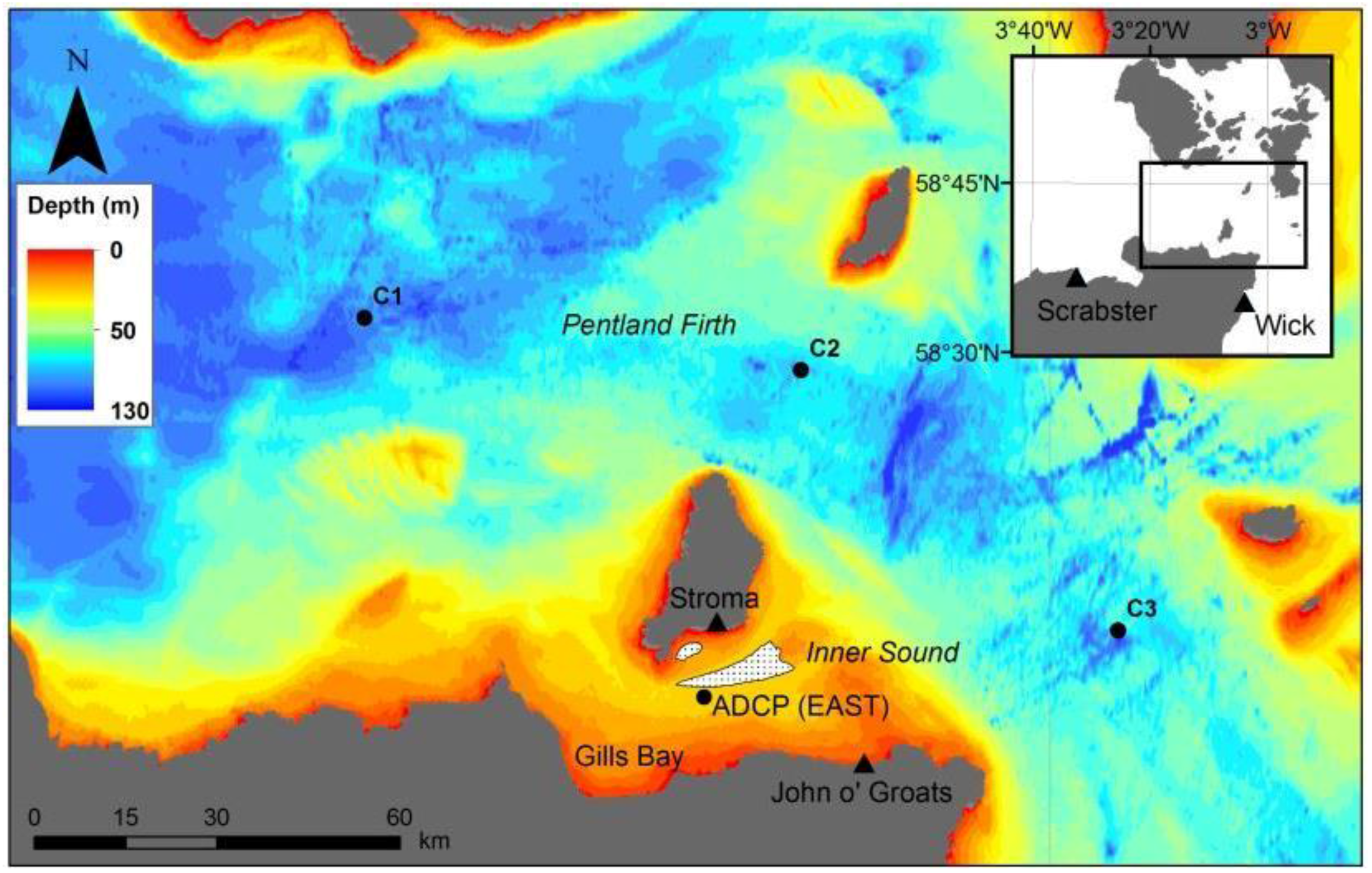
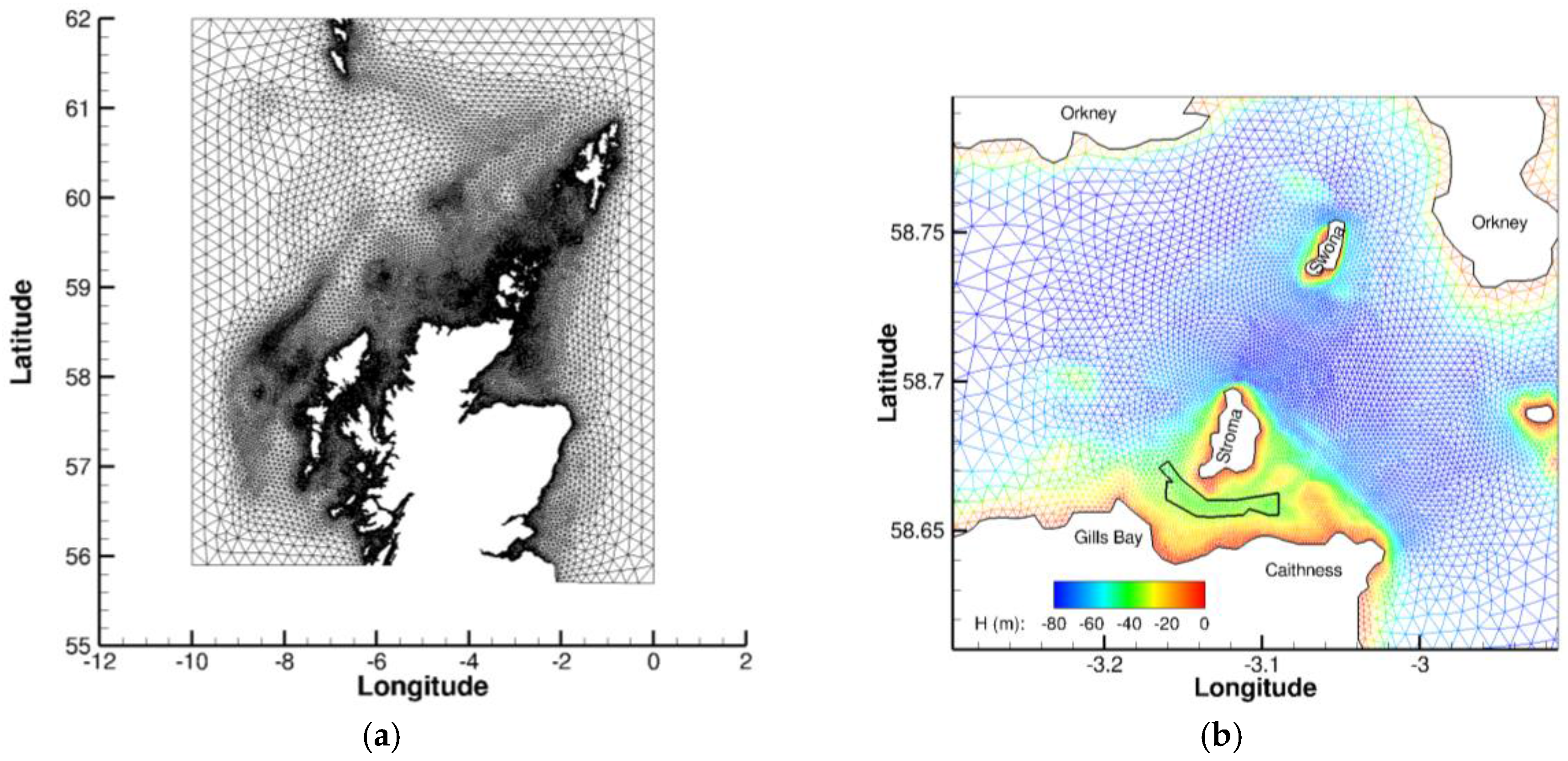
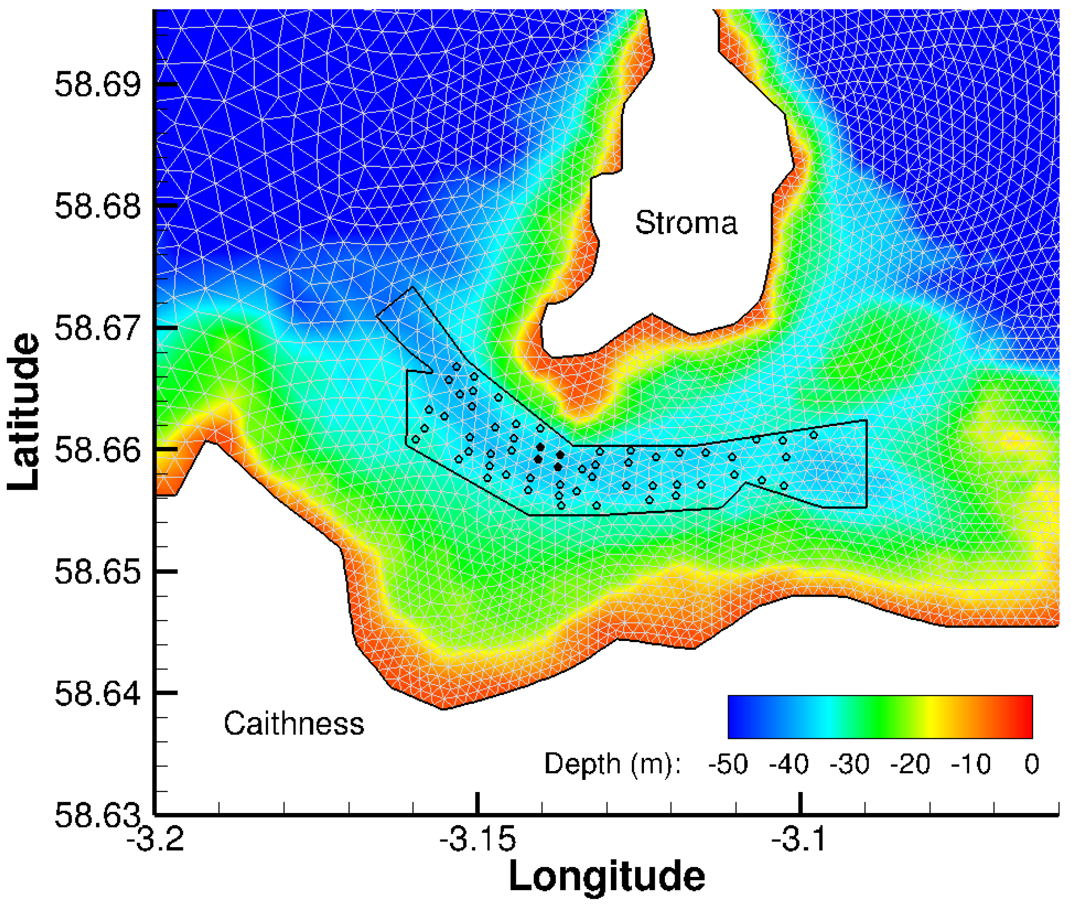
12]. Sediment banks are known to lie to the south of the island of Stroma (Figure 1) but the local sediment dynamics, and the potential impacts of tidal energy extraction on the deposits, are only beginning to be understood. McIlvenny et al. [11] suggested that the local sediment banks in the Inner Sound (Figure 1) have been locked in place for a significant period of time, with rates of sediment erosion and deposition expected to be low over the period. The tidal current velocities and the bed shear stress fields calculated by McIlvenny et al. [11] using a 2D hydrodynamic model were largely consistent with the observed sediment distributions, with sediment banks lying adjacent to the main flow through the Inner Sound. However, as with [8], the depth-averaged modelled velocities used by McIlvenny et al. [11] cannot be considered ideal to calculate bed shear stress fields.
Understanding of the tidal flow through the Pentland Firth and its subsidiary channels has advanced in recent years, due in part to the proliferation of numerical (e.g., [1,2,8,9,13], etc.) and observational studies (e.g., [14]). The strong flows through the Firth are generated from the hydraulic pressure head that forms across the channel due to the restriction placed on the propagation of the tide [13]; in order to capture the forcing of the flow through the Firth, it is necessary to accurately simulate the regional tidal regime. Most of the previous modelling studies have focused on the flow through the wider Pentland Firth, whereas in this paper we specifically consider the flow through the Inner Sound. The development of accurate and robust hydrodynamic models of the region is particularly important at present in order to predict potential effects on the ambient environment of tidal energy extraction prior to the deployment of large scale arrays.
In this paper, we investigate the potential effects of the development of a tidal turbine array on the bed shear stress in a tidally energetic channel: the Inner Sound of the Pentland Firth. Bed shear stress is a key parameter in the erosion of seabed sediment, and understanding potential implications of tidal energy developments on local sediment dynamics requires first an estimate of possible changes to the bed shear stress. Building on the 2D modelling work reported by McIlvenny et al. [11], we extend the modelling study to three dimensions, thereby resolving the vertical structure of the flow; we expect this to improve the estimates of near-bed velocity and therefore local bed shear stress during flood and ebb tides, and to allow better predictions of the potential changes to bed shear stress following the installation of tidal turbines in the region. In the following sections, we briefly describe the formulation of the model, including the parameterization of tidal turbines, and verify its performance against observations of sea surface height (SSH) and tidal current velocity. Results from simulations examining the effects of tidal turbines on velocity profiles, near-bed velocity fields and local bed shear stress are then presented. In the final sections, the results are discussed and some conclusions drawn.

2. Methods

2.1. Study Site

Our study site is the Inner Sound, lying between the Island of Stroma and the north coast mainland of Scotland (Figure 1). The channel forms the southern arm of the Pentland Firth, which lies between the Orkney Islands and the Scottish mainland and connects the North Sea to the North Atlantic. The Inner Sound is the location of one of the first deployments of commercial tidal turbines by Meygen Ltd. (Edinburgh, UK), with the first turbines expected to be in the water during 2016. In the first phase of the Meygen project, deployment of up to 61 turbines generating 86 MW has been consented [3]. Water depths in the Inner Sound reach about 36 m in the central channel. Shields et al. [4] described the Pentland Firth as comprising predominantly of exposed bedrock, but localised sediment and shell deposits around Stroma have been mapped in recent years [3,11,12]. An oval-shaped sediment bank lies immediately to the south of Stroma, and a wedge-shaped bank of shell fragments lies just adjacent to the main flow through the channel (Figure 1).
Both observations and hydrodynamic modelling have demonstrated the asymmetry in the tidal current regime through the Inner Sound. Flood tide currents entering the Sound from the west are diverted into the centre of the channel by the headland at the south-western extremity of Stroma. The main flow is accelerated around the headland, forming a stream about 1 km wide through the channel wherein current speeds at spring tides regularly exceed 4.5 m·s−1 (and have been recorded at up to 6 m·s−1) to the south of Stroma. Vessel-mounted acoustic Doppler current profiler (ADCP) surveys have shown similar features [14]. Modelling results suggested the presence of a trapped counter-eddy developing in the bay on the south coast of Stroma, at the location where the oval sand bank has been observed [11]. On the ebb tide, flows accelerate through the channel, with fastest speeds occurring to the south-west of Stroma. The ebb stream through the Inner Sound is shifted slightly north compared to the flood stream, since the headland at the south-east corner of Stroma does not protrude so far into the channel. In the central Inner Sound, current speeds during ebb tide are significantly less than during flood, and are orientated to the south-west rather than directly west. Maximum bed stress in the channel is therefore likely to be determined predominantly by the flood tide velocity field [11].
Bed stress values predicted using the two-dimensional (2D) hydrodynamic model ranged from about 0.5 Pa beneath the trapped eddy in the bay on the south coast of Stroma to values exceeding 50 Pa in the central channel and higher (>60 Pa) off headlands and in the main Pentland Firth north of Stroma [11]. Flood tide bed stress values less than 1 Pa might be expected to be associated with medium or coarse sand deposits [8], and the acoustic sonar survey reported by McIlvenny et al. [11] found evidence of such deposits. The 2D model simulations also suggested that the flood tide counter-eddy in the bay is a persistent feature and that the bank is also protected from the ebb tide currents by the headland to the east. To the south of the eddy, predicted bed stresses increased rapidly into the central channel [11].

2.2. Observations

2.2.1. Sea Surface Height Data

SSH data were collected at Scrabster and John O’Groats using WLTS 3791A instruments (Aanderaa, Bergen, Norway) set to record at 10 min intervals. Nominal instrument accuracy is 0.02 m. SSH data at Stroma were collected using a TideMaster (accuracy 0.01 m, Valeport, Totnes, UK), again with a sampling interval of 10 min. Data from the Inner Sound were obtained from a pressure sensor on the ADCP (see next section) with a 2 Hz sampling frequency; the data were reduced to ten-min averaged values before being analysed. Sea level at Wick is routinely measured for the UK National Tide Gauge Network, part of the National Tidal and Sea Level Facility; the hourly data used here from 2011 were obtained from the British Oceanographic Data Centre. Details of the data used are given in Table 1. Tidal analysis on the data was performed using the T-Tide software [15].

2.2.2. Acoustic Doppler Current Profiler (ADCP)

A 300 kHz upward-looking Workhorse ADCP (Teledyne, (Thousand Oaks, CA, USA) was deployed in the Inner Sound from February–March 2013 (Table 2). The instrument was deployed in about 36 m of water to the south of the island of Stroma (Figure 1) and sampled at 2 Hz, with data subsequently averaged into 1-min mean values. Bin size was 2 m. Valid data extended from approximately 6.5 m–30.5 m above the seabed. Tidal analysis on the velocity data was again performed using the T-Tide software [15].
In 2001, three ADCPs were deployed at locations in the Pentland Firth by Gardline Ltd. (Great Yarmouth, UK) [16] (Table 2). Results from a tidal analysis of the data were used in this study, with constituent values for near-surface, mid-depth and near-bed bins presented. Some uncertainty in the reliability of the results of the Gardline ADCP data have been noted, due to reported “knock down” of the mooring lines during the fastest flood and ebb currents [9,17]. As a result, we place more emphasis on the phase of the observed currents than on the amplitude in the calibration of the model.

2.3. Hydrodynamic Model

2.3.1. Mathematical Framework

The numerical model River and Coastal Ocean Model (RiCOM) is a general-purpose hydrodynamics and transport model, which solves the standard Reynolds-averaged Navier-Stokes (RANS) equation and the incompressibility condition, applying the hydrostatic and Boussinesq approximations. It has been tested on a variety of benchmarks against both analytical and experimental data sets (e.g., [18,19,20]). The model has been previously used to investigate the inundation risk from tsunamis and storm surge on the New Zealand coastline [19,21,22], to study tidal currents in high energy tidal environments [23] and, more recently, to study tidal energy resource [24,25,26] and the effects of energy extraction on the ambient environment [11].
The basic equations considered here are the three-dimensional (3D) shallow water equations, derived from the RANS equations by using the hydrostatic assumption and the Boussinesq approximation. The continuity equation for incompressible flows is:
u + w z = 0
where u(x,y,z,t) is the horizontal velocity vector, w(x,y,z,t) is the vertical velocity, is the horizontal gradient operator, and z is the vertical coordinate. The momentum equation in non-conservative form is given by [25]:
D u D t + f z ^ × u + g η z ( A V u z ) ( A h u ) + F = 0
where t is time; f(x,y) is the Coriolis parameter; z ^ is the upward unit vector; η(x,y,t) is the sea surface displacement relative to mean sea level; g is the gravitational acceleration; AV(x,y,z,t) and Ah(x,y,z,t) are the vertical and horizontal eddy viscocities respectively; F represents body forces including form drag from obstacles in the flow; and x, y are the horizontal coordinates aligned to the east and north respectively.
The free surface equation is formed by vertically integrating the continuity equation and applying the kinematic free surface and bottom boundary conditions:
η t = ( h η u d z ) = 0
where h is the water depth relative to the mean level of the sea.
In the simulations reported here, the model was run without an applied surface stress. At the seabed, a slip condition with quadratic stress is applied i.e., the seabed stress, τb is given by:
τ b = ρ C D u b | u b |
where ρ = 1025 kg·m−3 is the water density, and CD is a drag coefficient and ub is the near-bed velocity. The value of CD is varied during calibration to provide the best fit to observations of sea level and velocity.
The equations are discretized on an unstructured grid of triangular elements which permits greater resolution of complex coastlines. The momentum and free surface equations are solved using semi-implicit techniques to optimize solution time and avoid the CFL stability constraint [26]. The material derivative in (2) is discretized using semi-Lagrangian methods to remove stability constraints on advection [27,28]. The Coriolis term is solved using a 3rd order Adams-Bashforth method [29]. Full details of the model discretization and solution methods, including the basis of the application to tidal energy, are given elsewhere [25,26]. The solution methods provide a fast, accurate and robust code that runs efficiently on multi-core desktop workstations with shared memory using OpenMP (http://openmp.org/).

2.3.2. Configuration and Boundary Forcing

The model grid covered the northern Scottish continental shelf (Figure 2). The unstructured mesh varies in resolution, with element side lengths decreasing from 20 km at the outer boundaries of the model to ~50 m in the Inner Sound. In the vertical, sigma coordinates were used with 15 sigma levels at σ = [0.00, −0.02, −0.05, −0.10, −0.15, −0.20, −0.30, −0.40, −0.50, −0.60, −0.70, −0.80, −0.90, −0.95, −1.00]. In total, the 3D model grid contains 2,351,104 nodes and 1,044,914 triangular elements.
The model was forced at the outer boundaries by seven tidal constituents (O1, K1, Q1, M2, S2, N2, M4) which were taken from the Oregon State University (Corvallis, OR, USA) global tide model [30]. No wind forcing was applied and water density was assumed to be constant. Bathymetry was obtained from a variety of sources, amalgamating sources of increasing resolution closer to the coast. Within the Pentland Firth itself, bathymetry was extracted from multibeam sonar survey data. The model was spun up for two days from 16 to 18 February 2013, with the main simulation running from 18 February to 24 March 2013.
For the present simulations, the vertical viscosity, AV, was defined using a law of the wall formulation with a double length scale from the bottom and the surface, i.e.,:
A V = κ | u | [ ( z + z 0 ) ( 1 z h ) + z s z h ]
where κ is the von Karman constant (κ = 0.4), u is the friction velocity ( u = (τb/ ρ )½), and z is the height above the seabed. The length scale parameters were set to z0 = zs = 0.1 m. The horizontal viscosity term, Ah, was not used. The model time step was 36 s. On a desktop computer with 8 cores using OpenMP, the model took 8 h to run the 34 day simulation (i.e., 102 times faster than real time).

2.3.3. Calibration

Results were calibrated against the SSH data from Scrabster, Wick, Stroma, John O’Groats and the Inner Sound (as described above). Calibration was performed by varying the drag coefficient CD through a range of values from 0.002 to 0.010 and performing a tidal analysis on the resulting SSH time series from the five locations. Results of the calibration exercise are presented in Section 3.
Tidal velocity predictions from the model were evaluated against the four deployments of ADCPs in the Pentland Firth and Inner Sound during 2001 and 2013. Predictions from near-surface, mid-water and near-bed are presented. As noted above, for the Pentland Firth sites the calibration exercise placed more emphasis on constituent phase than amplitude, due to concern about possible effects of mooring “knock down”.

2.3.4. Parameterisation of Tidal Turbines

Tidal turbines are represented in the model by introducing a form drag into the momentum Equation (2). The derivation of form drag through double-averaging methods is described elsewhere [26,31,32]. Here we assume that form drag is introduced to represent subgrid scale obstacles in the flow, with the solid object comprising a fraction of the grid cell volume. We assume that power is generated uniformly over the face of the turbine such that power is defined by the average speed over the turbine area, which in our case is represented as the current speed averaged over the volume of a computational cell. The power generated, P, is then given by:
P = 1 2 ρ A T C P U R 3
where UR is a reference current speed. The form drag is defined as:
F D = 1 2 ρ A T C T | U R | U R
In (6) and (7), AT is the frontal area of the tidal turbine normal to the direction of flow, CP is a power coefficient, CT is a thrust coefficient and UR is a reference current velocity.
The difficulty within an ocean model context in choosing a suitable value for the free stream velocity in the vicinity of a tidal turbine has been discussed elsewhere (e.g., [26,33,34,35]). This is particularly true in real world simulations involving complex coastlines where the flow field is highly spatially variable. One approach has been to use a volume-averaged velocity, U, from the model and to adjust the values of CT and CP to account for the discrepancy between U and UR [26,33,34]. Walters [26] tested three approaches to addressing the discrepancy between reference and volume-averaged velocity, one iterative method and two mapping formulations, and achieved similar estimates of thrust and power generation with each. Here, we used a simpler approach, by specifying a relatively large averaging volume such that U approximated UR.
In a three-dimensional model, the form drag must be distributed within the water column across the depth range occupied by the tidal turbine. The dimensions of the averaging volume to calculate U need to be specified, and need not be limited to the scale of the turbine [33]. Here, we define the averaging volume to be the size of a computational cell in the horizontal, and twice the diameter of the turbine blade in the vertical. Given that the turbine blades have a diameter of 18 m, the vertical extent of the averaging volume is 36 m which is approximately the total water depth in the Inner Sound. For consistency, it is also necessary to ensure that the volume-averaged form drag is equivalent to the form drag calculated using the volume-averaged velocity [26]. In addition, the specification of form drag in the present model is further complicated because the drag is calculated on the element sides, whereas velocity is averaged over elements. To satisfy these criteria, the form drag at each sigma layer is therefore approximated by:
F K = 1 2 ρ A K C K | U | u K
where the subscript K indicates parameter values at the Kth vertical layer, AK is the frontal area of the turbine at level K, uk is the velocity at layer K, and CK is the thrust coefficient that is adjusted for each layer so that the volume-averaged form drag is equal to the value based on the volume-averaged velocity. The inclusion or exclusion of each vertical layer in the area swept by a turbine blade must be determined for each turbine based on the blade diameter, water depth and vertical height of the turbine hub in the water column. These parameters must be supplied to the model through the input file.
Using (8) to simulate the form drag imposed by a tidal turbine allows the model to confine the resultant thrust to the part of the mid-depth water column which is swept by the turbine blade, and allows the model to simulate the flow underneath and above the swept area. This is particularly important since we are investigating effects on the bed shear stress which is determined by the near-bed flow.
Power is calculated simply by replacing the reference speed in (6) by the volume-averaged current speed, i.e.,:
P = 1 2 ρ A T C P U 3
Two approaches were tested for assigning values to CT and CP. First, constant values of CT = 0.8 and CP = 0.42 were used, following Bahaj et al. [36]. This approach does not incorporate cut-in or cut-out velocities, with the coefficients applied uniformly at all flow velocities. The resulting thrust and power curves for a range of current speeds are shown in Figure 3. The second approach used the flow-dependent thrust coefficients proposed by Baston et al. [37] as part of the TeraWatt project. In this case, cut-in and cut-out speeds of 1 m·s−1 and 4 m·s−1 respectively were applied. Each turbine was given a rated power of 1.5 MW at a current speed of 3 m·s−1; at speeds greater than 3 m·s−1, the value of CP was decreased according to (6) so that power generation remained constant at 1.5 MW at the higher velocities (see [24]) until velocities exceeded the cut-out speed. The profiles of CT and CP with current speed and the resulting thrust and power curves are also shown in Figure 3. The TeraWatt power and thrust curves are believed to be reasonably realistic curves for a generic tidal turbine [37].
Simulations were performed using both sets of power and thrust coefficients, and the results compared to simulations without turbines present (Table 3). A virtual array of 57 tidal turbines, each rated to 1.5 MW, was introduced into the lease area within the Inner Sound (Figure 2). This amounts in total to the consented 86 MW for the entire array. The locations of the individual turbines were distributed evenly but arbitrarily over the lease area (Figure 4). No more than one turbine was located in any single grid cell. Each turbine had a blade diameter of 18 m, and the hub was situated 15 m above the seabed. Each turbine was assumed to have a yaw mechanism and face into the flow at all states of the tide. Form drag due to the support structure was not modelled, as it is relatively insignificant compared to the turbine thrust itself [24].

2.3.5. Model Output

The three-dimensional velocity fields were saved every hour over the 34 day simulation from 18 February to 24 March 2013. Power output at each turbine location and the total power generated by the array was also calculated and stored every hour. The maximum velocity that occurred at each grid point over the duration of the simulation was also stored. From these stored velocity fields, values of bed shear stress were calculated using τ b = ρ C D | U R | U R (only the magnitude of the bed shear stress is considered here). Near-bed velocities, Ub, were taken from the bottom sigma layer, which had a mid-layer height of 2.5% of the water depth; with maximum channel depths of ~36 m in the Inner Sound, the near-bed velocities were typically within 1 m of the seabed. For the bed shear stress calculations, the value of CD derived during the calibration process (CD = 0.004) was used.
By calculating the difference in the results from the simulations with turbines (Runs 2–7) to the baseline simulation (Run 0), the effects of the presence on the turbines to the near-bed current fields and local bed shear stress can be examined. All difference plots are calculated by subtracting the baseline (Run 0) from the results with turbines i.e., a positive difference means the turbines increase the value of the variable.

3. Model Calibration and Evaluation

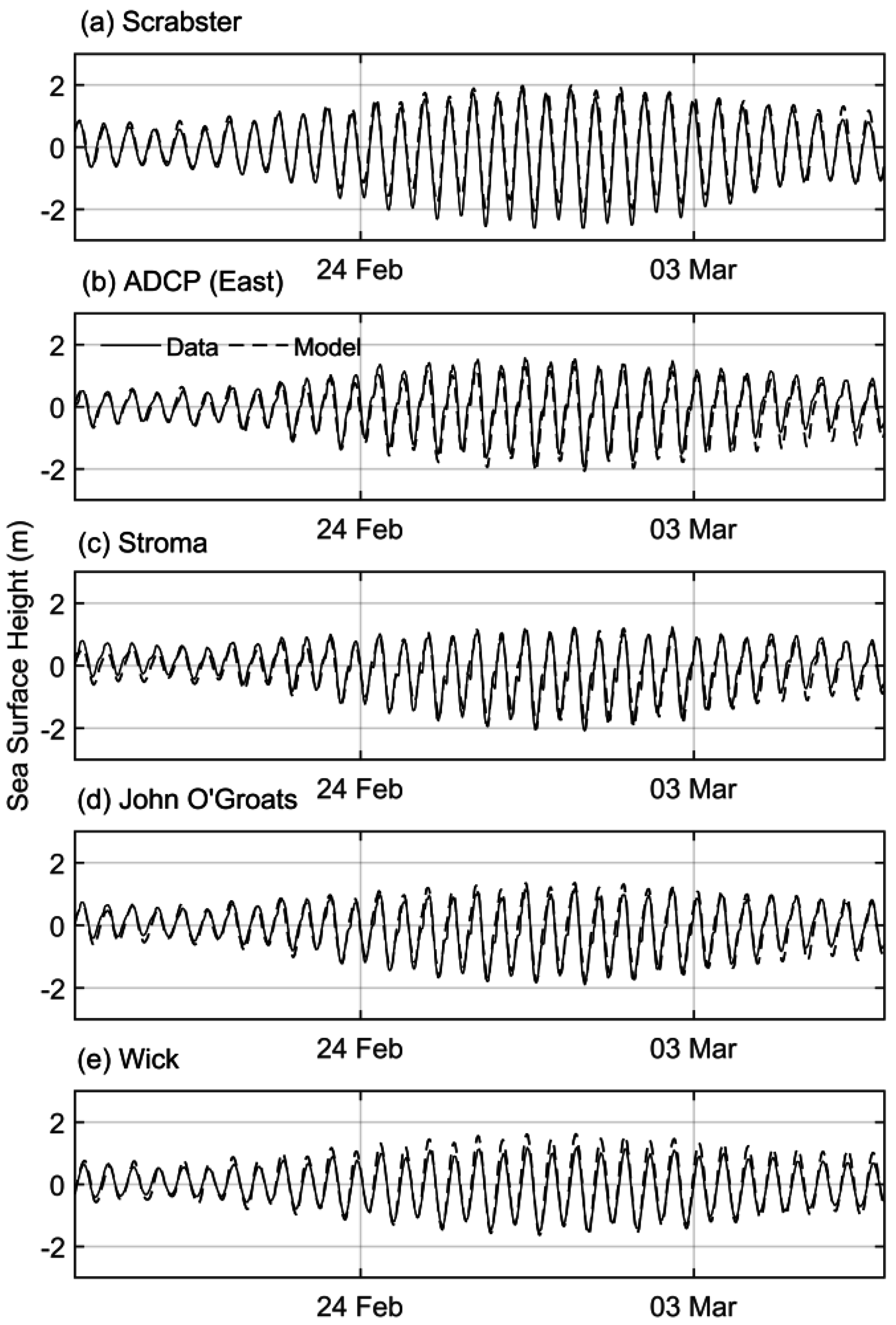
The hydrodynamic model accurately reproduced the tide at tide gauge locations around the northern Scotland coastline, including both ends of the Pentland Firth, capturing the change in amplitude and phase of the tide that occurs through the Firth (Figure 5). This is a minimum requirement for the model to be fit-for-purpose, since currents in the Firth are largely driven by sea level pressure gradients [13]. We varied the frictional drag coefficient, CD, over an order of magnitude range, 0.002 ≤ CD ≤ 0.01. Overall, the best agreement was achieved with mid-range values, although no single value produced the best results at all locations. The model results reported in the remainder of this paper are from the simulation with CD = 0.004, similar to values used in other studies (e.g., [13]).
Tidal analysis confirmed that the modelled amplitudes of the dominant M2 constituent were typically within ±0.04 m (<5%) of the observed values, with the exception of John O’Groats, where the discrepancy was 0.10 m (Table 4). Modelled phases for the M2 tide were within 3° of the observed values at all locations. The model captured the sharp change in M2 phase across the Pentland Firth.
For the smaller constituents, model-data discrepancies in both amplitude and phase were slightly larger as the errors in the tidal analysis increased due to the relatively short time series (34 days). Errors in the amplitude of the S2 tide were generally less than 0.03 m, except against the ADCP measurements, and errors in the S2 phase were less than 10°. For N2 and the diurnal constituents, the modelled amplitude was within 0.04 m and the modelled phase generally within 10° of the observed values. Interestingly, the discrepancies in the modelled phases of the K1 constituent at Stroma and the ADCP location (both within the Inner Sound) were larger, although good agreement was achieved at the surrounding locations.
Calibration of the model was based on SSH, with the performance of the model with the selected value of CD = 0.004 then assessed by comparing the modelled velocities against moored ADCP data. The comparison showed acceptable levels of agreement in the magnitudes and phases of velocity for the principal tidal constituents (Table 5), particularly given the uncertainties in the Gardline ADCP data from the Pentland Firth. The M2 tidal constituent dominated both the regional tides and particularly the local tidal currents in the Inner Sound, being 2.5 times stronger than the next largest constituent S2 (Table 5). Errors in the amplitude of the dominant East component of the M2 constituent were of the order of 20% of the observed amplitudes. For the Inner Sound ADCP data, however, the quality of which is more certain, the model error was less than 5% of the observed amplitude. This is important since our focus in this paper is on the Inner Sound. In terms of phase for the eastward M2 velocity, the modelled tide led the data by 6° at the Inner Sound ADCP; the average difference between model and observations over all sites including the Gardline data was 4° (Table 5). This is very good agreement for the dominant tidal component.
For the northward component of M2 velocity, relative errors were larger since the amplitude of the component is much smaller than the eastward velocity. In particular, at C1 and the ADCP location, the amplitudes of the northward component were only about 5% of the eastward component. The model performed better at C2 and C3, where the amplitude of the northward component is comparable to the eastward. The modelled phases also compared much better at C2 and C3. The flow through the Pentland Firth, and through the Inner Sound in particular, is highly dynamic, turbulent, and strongly steered by local topography. The high spatial variability in the flow makes comparison between modelled and predicted currents difficult, particularly in the cross-flow direction; in these regions of highly sheared flow, small changes in location of the model output can substantially affect the error estimate. We have not, therefore, placed a strong emphasis on the northward component of velocity in the calibration exercise.
For the smaller S2 constituent, average modelled errors were larger than for M2, with average modelled amplitude errors of 26% of the observed amplitude. The phase of the eastward S2 constituent had an average error of 9° (Table 6), and only 3° in the Inner Sound. Like the M2 constituent, the northward component of S2 had large relative errors for the small amplitude tide, and larger errors in phase at C1 and C3; the S2 phase at C2 and the Inner Sound were modelled reasonably well.
Given the good model performance for SSH and the uncertainty in the observed current data, the model performance is acceptable. Further refinement of the model is expected as more observational data, from additional ADCP deployments and surveys and deployment of an X-band radar system, become available.

4. Results

4.1. Near-Bed Velocity Fields

Maps of the peak velocity through the Pentland Firth and Inner Sound, during both the flood and ebb phases of a spring tide, illustrate the strength of the tidal flow in the area (Figure 6). The velocity vectors and current speeds shown are the near-bed currents, from the bottom model sigma layer, typically representing modelled currents 1–2 m above the seabed. During spring flood tide, modelled near-bed current speeds through the Inner Sound reached 5 m·s−1; flow was focused in the central channel through the Inner Sound. Similarly, in the wider Pentland Firth, to the north of Stroma, near-bed velocities reached 5 m·s−1 at peak flows. Areas of weaker flow are evident in the lee of the island of Stroma. The presence of the island leads to areas of very strong current shear, particularly to the south of the island, where peak currents increase from less than 1 m·s−1 to over 4 m·s−1 over a distance of the order of 100 m. Anecdotal evidence for this strong shear zone come for the intensive present of seabirds, which have been observed aligned along the front (Helen Wade, personal communication).
On the ebb tide, current flows are still very strong, but not quite as intense as on the flood tide. The eastern entrance to the Inner Sound is wider than the western entrance, and the modelled flow through the channel was also therefore wider. The current shear was slightly weaker, and the main flow came closer to the southern shore of the island. Weaker flow in the lee of the island was again evident, and low flows were apparent in the bays on the mainland.
As might be expected, sediment distributions in the Inner Sound appear to be closely linked to these hydrography [11], with sand and shell banks located adjacent to the main flood current (Figure 1). Given the sharp lateral gradients of current strength, deposition and erosion of these sediments might be expected to be quite sensitive to changes to the present flow regime.

4.2. Turbine Effects on Velocity Profiles

Simulation-mean current profiles at the four turbine locations from Runs 4 and 5 exhibited a classical tidal velocity profile (Figure 7). Mean current speeds in the Inner Sound lie in the range 2.0–2.5 m·s−1 in the top 30 m of the water column. Below 30 m depth, the mean velocity falls away rapidly to about 1.5 m·s−1 just above the seabed. This profile is evident at all four locations, and compares well with the mean velocity profile measured nearby by the ADCP.
Turbines occupied the water column from 6 to 24 m above the seabed (the turbine hubs were located at 15 m above the seabed). The flow was clearly retarded by the presence of the turbines, with the greatest impedance evident at mid-depth. Above and below the turbine, the flow was less affected by the presence of the turbine, but the mean current strength was still weaker than predicted in the absence of turbines. These profiles do not have the large velocity deficit at the turbine and the accelerated flow beneath the turbine predicted by computational fluid dynamics (CFD) models e.g., [38] because the velocities are volume-averages. However, previous work [33] has shown that the averaged velocities from a CFD model are very similar to the averages derived by the larger scale model used here.
The thrust exerted by the Bahaj et al. algorithm [36] is not limited as flow speeds increase above the rated velocity; consequently much greater thrust is imparted on the flow than for the Baston et al. [37] algorithm, and retardation of the flow is more pronounced. Given that current speeds quite regularly exceed the rated velocity of the turbines at spring tides, it seems likely that using the Bahaj et al. algorithm is likely to overestimate the impact of the turbines on the flow. As such, the following sections consider the effects of turbines on the flow using the Baston et al. algorithm only.

4.3. Turbine Effects on Near-Bed Velocity Fields

The effects of a single turbine (Runs 2 and 3) and an array of four turbines (Runs 4 and 5) on the ambient dynamics were small. The larger array of 57 turbines, however, produced clearly discernible effects, on both flood and ebb current regimes (Figure 8). Note that these are near-bed velocities, on which the turbine presence has a lesser effect than on mid-water current speeds. Even so, a general pattern of reduced current within and downstream of the area of the array and accelerated flow around the edges of the array is evident. On the flood tide, increased current speed was evident along the northern edge of the array, with velocities increased by up to 0.8 m·s−1 in small areas. Current speeds were also slightly increased to the south of the array. The retardation of the flow was more widespread, affecting current speeds within the array but extending downstream for many kilometers. Interestingly, small increases in flow speed off the northern tip of Stroma are also evident.
On the ebb tide, the changes in current speed are even more marked. Again, flow within the array is reduced and that reduction extends several kilometers downstream, and there is an area of increased flow along the northern perimeter of the array lease area. Most noticeably, however, is the large area in the lee of Stroma where the turbine array appears to increase the ebb current speed. This occurs because of a small shift in the position of the ebb tide jet emerging from the western end of the Inner Sound, which strengthens the gyre circulation in the lee of Stroma.
The maximum current speed at every model location over the course of each simulation was also recorded. Maximum values may occur at different times in different simulations, but maximum current speeds are likely to determine sediment deposition and erosion and are therefore of interest here. The difference in maximum near-bed speed between Runs 7 and 1 (Figure 8) shows a complex pattern of change when turbines are introduced into the flow. The largest changes in near-bed maximum speed occurred to the east of the array–here a shallow ridge extends northward from the mainland coast and, coupled with the turbine array, evidently affects the flow speeds. Within the array lease area, maximum near-bed current speeds are generally, but not entirely, reduced. To the west, areas of reduced and increased maximum flow induced by the turbines are evident; as noted above, this appears to be related to a shift in location of the ebb tide jet, and modification of the gyre circulation behind Stroma as a result. Clearly, the introduction of an array of 57 turbines has the potential to modify the near-bed velocity field, with consequent effects on local bed shear stress.

4.4. Local Bed Shear Stress

Patterns of local bed shear stress (Figure 9) obviously exhibit the same broad scale features as the corresponding near-bed velocity fields, but being a function of the velocity squared some detailed features are enhanced. The increase in bed shear stress along the northern perimeter of the array lease area on flood tide reaches 8 Pa. As noted by [8], such a change is equivalent to a change in sediment type from medium sand to fine gravel. This band of increased stress coincides with the established shell bank [11]. Downstream of the array, bed stress values are much reduce, again by up to −8 Pa, this time corresponding to an equivalent shift from fine gravel to medium sand. The marked effects in bed stress extend to the Ness of Duncansby at the north-east tip of Caithness, some eight kilometres east of the array.
On the ebb tide, as for the near-bed velocity, marked changes to the bed stress are predicted for the area behind Stroma. Along the northern periphery of the array area, increases in predicted bed stress exceeded 5 Pa; in small areas, this may be equivalent to a shift from medium sand to medium gravel. The difference in maximum bed stress between the two simulations (Run 1 and Run 7) was not as strong as the direct comparison between contemporaneous bed stress values from the two simulations.

4.5. Power Generation

Since the purpose of tidal turbines is to generate power, we briefly consider the power produced by the simulated turbine arrays. Power was calculated at each turbine location, and then summed over the array. The mean power per turbine was then calculated. Power per turbine is clearly a function of the size of the array, as has been noted elsewhere [39]. Here the smaller arrays with one and four turbines produced almost 100% of the expected energy (Figure 10). The array of four turbines experienced a slight drop-off as the cut-out velocity (4 m·s−1) was reached, whereas the single turbine exactly reproduced the theoretical power generation.
For the larger 57-turbine array, the mean power only briefly reached the rated power, when the array-averaged velocity exceeded the rated velocity (3 m·s−1). As the velocity increased further, the power per turbine dropped significantly, from 1.5 to 0.5 MW. This was evidently due to blockage effects from the array itself. It is also notable that the maximum array-averaged velocity was significantly less for the large array, reaching only 4.4 m·s−1; the velocity for the 1- and 4-turbine arrays reached 5 m·s−1.
The power generated using the algorithm by Bahaj et al. [36] produced much more power at higher velocities (Figure 10), but as noted above, the lack of a cut-out velocity in the algorithm as applied here is not considered particularly realistic and the power curves are therefore unlikely to be achieved.

5. Discussion

Ongoing concerns about possible environmental effects of large arrays of tidal turbines on the marine environment and ecosystem need to be addressed in order to ensure that the fledgling marine renewable energy industry can develop and meet its potential in a sustainable manner. The current absence of real world commercial tidal arrays means that accurate and robust hydrodynamic models are an important tool to predict potential effects on the ambient environment prior to array development. Here we have explored the performance of a three-dimensional hydrodynamic model that uses finite element solution techniques on an unstructured grid to simulate tidal flows and turbine impacts through the Pentland Firth and Inner Sound, where tidal energy capacity is being actively developed [3]. The model reproduced the amplitude and phase of the surface tide accurately, capturing the change of both that occurs through the Pentland Firth. The agreement between modelled M2 currents was generally very good, particularly for the predominant eastward component. Errors tended to be larger for the comparison with the currents at C1; it is possible that the reported “knock down” of the mooring [9,17] was more of an issue at this site. However, the phase of the M2 current was very well modelled at all sites. Errors for the eastward component of the S2 tide were larger than for M2, although the phase was again accurately reproduced. The larger errors occur as the amplitude of the constituent is a much smaller component of the total signal, making the constituent harder to model. Again, the errors for site C1 were larger than at the other sites, raising questions over the reliability of the data at that location.
The northward components of both constituents were not as accurately reproduced as the eastward components, being generally significantly smaller in amplitude. In the Inner Sound, for example, amplitudes of the northward components were only about 13% of the eastward amplitude. The high spatial variability of the flows may also disproportionately affect the northward components in the model-data comparison. Overall, the calibration exercise demonstrated that the key elements of tidal flow through the region were well captured by the model.
The calibration exercise found that simulations with a drag coefficient of CD = 0.004 produced the overall best fit to the observations. This value is consistent with values used in other numerical studies of this area (e.g., [2,8,9,13]). However, the model was not highly sensitive to the drag coefficient used, with values in the range 0.003 ≤ CD ≤ 0.006 all resulting in acceptable model performance, accurately simulating the change in tidal amplitude and phase across the Firth.
The ability of the model to simulate tidal turbine effects using a form drag approach has been demonstrated previously [26,33], and the model has been applied in other locations to estimate potential marine energy generation [24,25]. Form drag from subgrid objects must be dealt with by integral methods to connect the subgrid scale with the model scale [26], but clearly, subgrid scale effects cannot be reproduced with this method. Other approaches to modelling tidal turbines in ocean models have been used (e.g., [
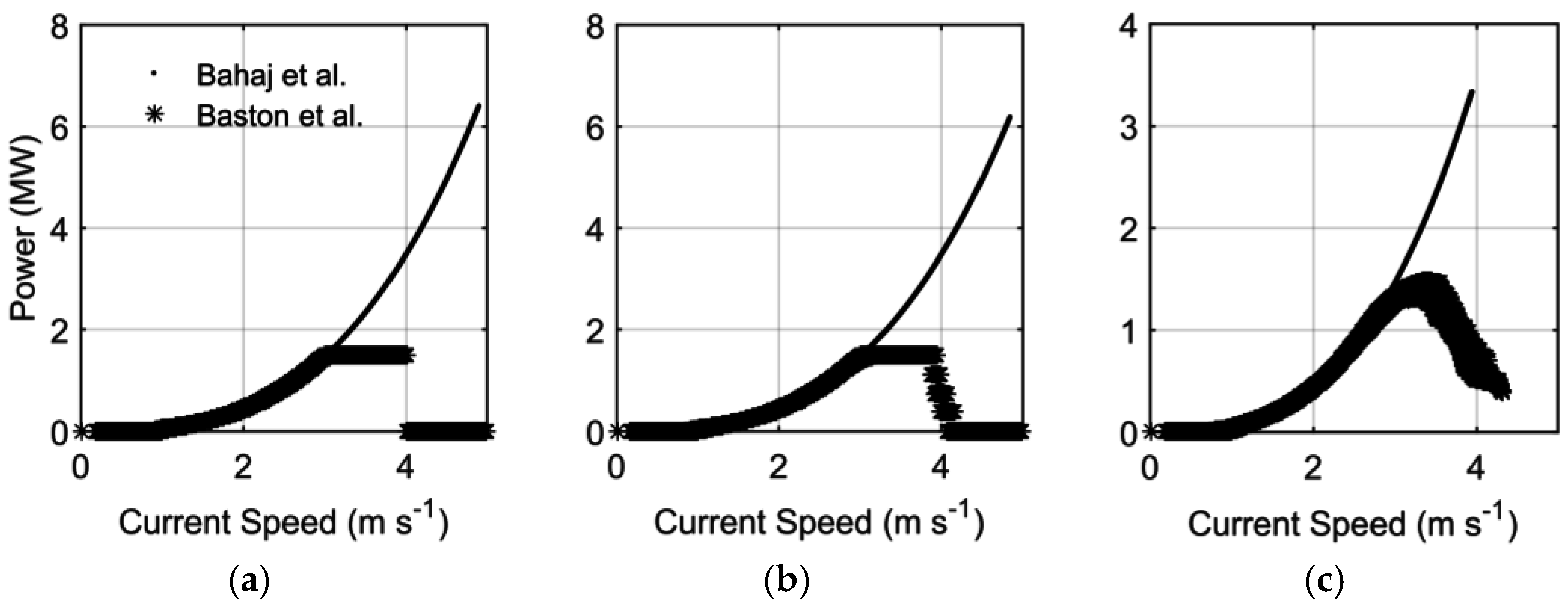
2]). Each approach poses challenges in terms of the choice of velocity used to calculate both the thrust imposed by the turbine on the flow and power generated. Actuator disc theory requires detailed information of the flow upstream from, downstream from and at the turbine location. The last of those is hard to obtain from an ocean model with, typically, much larger grid cell size than the scale of a turbine. The form drag approach, likewise, requires an approximation of local free-stream velocity in order to calculate thrust and power using (6) and (7), the specification of which is not obvious in complex real world tidal flows. Walters [26] tested three approaches to addressing the discrepancy between reference and volume-averaged velocity, one iterative method and two mapping formulations (one from [34]), and achieved similar estimates of thrust and power generation with each. For larger turbine arrays, the iterative approach is less attractive, but the mapping formulations appear to offer a promising solution to the problem. The approach employed here, using a relatively large averaging volume at the turbine location such that the averaged flow approximated the reference velocity, worked reasonably well and gave satisfactory results for power generation. However, future work will include testing of the mapping formulations to improve the representation of turbine drag in the model.
In the simulations reported here, the mean power generated per turbine fell as the size of the array became larger (Figure 10) as evidently the blocking effects of the array itself inhibited power generation at down turbines. The turbines modelled here were located arbitrarily with the lease area since likely locations are not known. Because the model does not reproduce the sub-grid scale details of turbine wakes, the power estimates were based on an implicit assumption that interactions between individual turbines were weak. The turbines were positioned at least a blade diameter apart and were not aligned, which should minimize wake effects. Dealing with wake effects in coastal ocean models (rather than CFD codes) is a matter of ongoing research. Array optimization has been the subject of considerable analytical and theoretical work (see [39] for a review), but less work through numerical modelling. Recent developments include the use of adjoint methods with a 2D model to optimize the locations of 256 turbines in a channel with steady flow [40]. That study found a solution for the optimal positions of the 256 turbines within 200 forward runs. An alternative approach is too simply run successive iterations of a numerical model, placing turbines iteratively at the location of highest velocity within the array area until the full array is position. For large arrays, such iterative solutions to find the best locations appear to present daunting computational demands, but the present model is fast and simplified 2D solutions could be attempted using this approach.
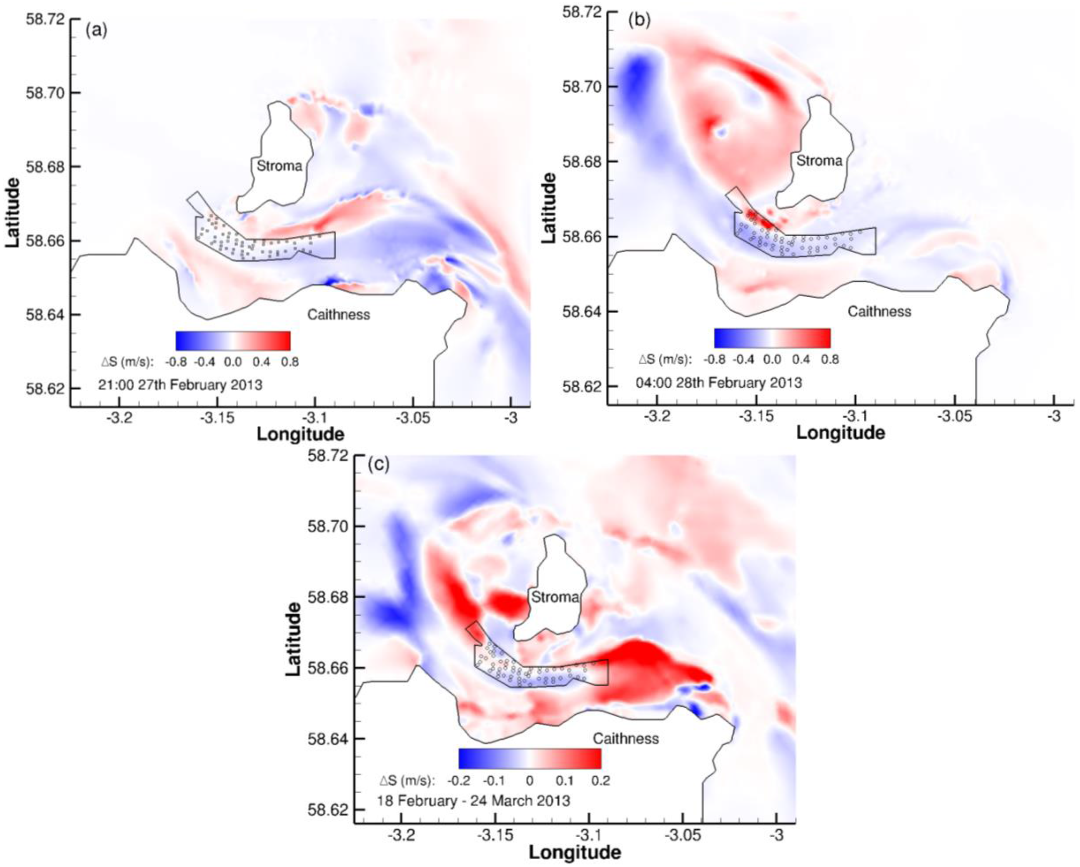
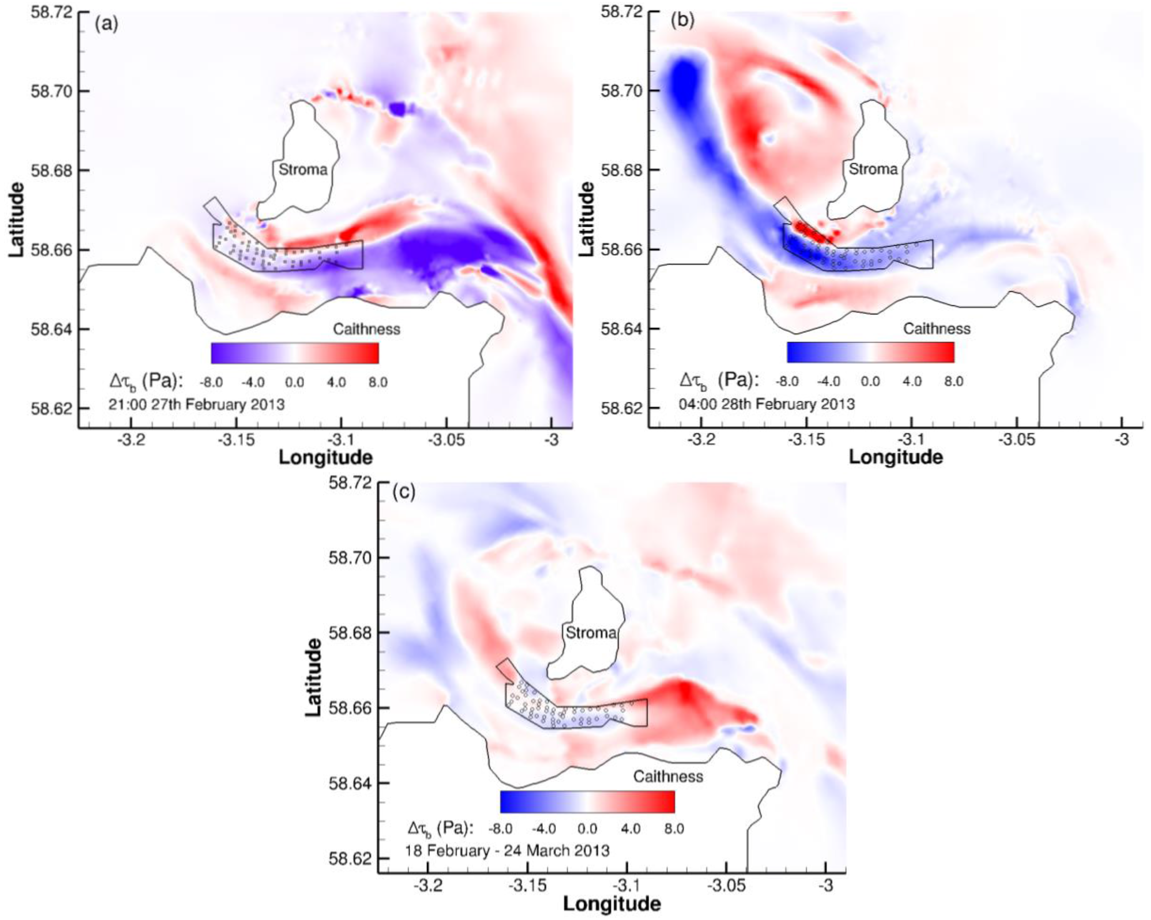
Deploying increasing numbers of turbines in the water column clearly proportionately modifies the ambient hydrodynamics. The effects of the small numbers of turbines (e.g., single turbines and a group of 4) modelled here were small; however, the larger array of 57 turbines produced some clear impacts on near-bed velocity and bed shear stress, not just at the location of the turbine array but over the local area for several kilometres. The enhanced stress predicted is enough to have significant effects on sediment type and is coincident with an established shell bank [11]. The shell fragments comprising the bank are not spherical but rather flat, and their depositional and erosional characteristics are not currently well known [11], so the effects of an increase in bed shear stress by up to 8 Pa is difficult to predict at present. However, ongoing monitoring of the shell bank [12] will provide valuable data for future modelling of similar banks in the region as tidal energy deployments proceed.
This zone of enhanced bed stress was not captured by modelling studies by Martin-Short et al. [8] and Fairley et al. [9], but otherwise our results were broadly consistent with theirs. Within and downstream of the array, velocities were reduced and broad bands of reduced bed stress extended downstream. Martin-Short et al. [
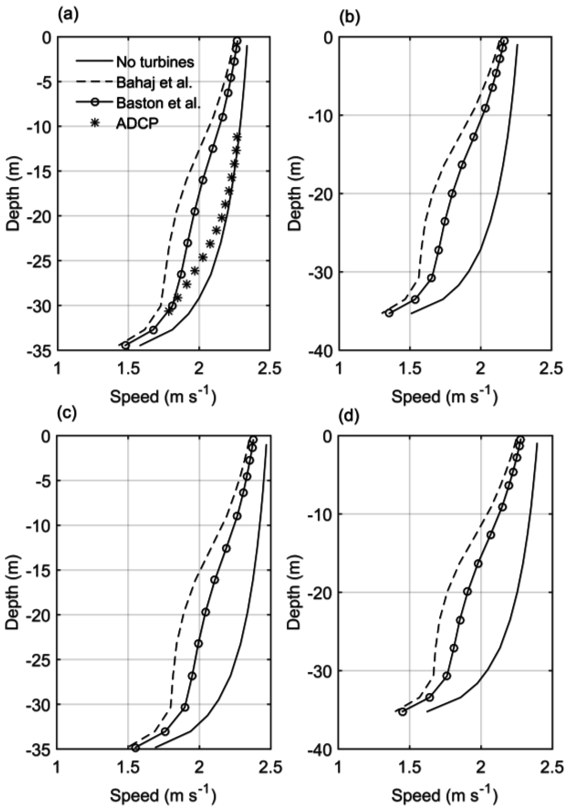
8] modelled the impacts of an array of 400 turbines and found bed shear stress changes of up to 25 Pa, peaking to the east of the array above the shallow ridge. They used a 2D model, whereas it is evident from the profiles of velocity that near-bed velocity is significantly reduced relative to the depth-averaged, and a 3D model is necessary to accurately predict bed stress. They found changes to the velocity field and bed shear stress extended up to 15 km from the array location, but their array of 400 hundred turbines extracted about five times more energy than our simulated array.
In contrast to the shell bank, the location of the oval-shaped sand bank in the bay on the southern shore of Stroma (Figure 1) was not predicted to experience significant changes to bed shear stress due to array development. The predicted values of Δτb above the sand bank were less than 1 Pa (Figure 10), which should have minimal impact. Monitoring both the sand and shell banks into the future could provide an interesting contrast in the influence of the array on local sediment features.
Fairley et al. [9] focused on two regions of sandy seabed in the vicinity of the Pentland Firth, one of which was the area of sandbanks found to the west of Stroma. These sandbanks consist of medium to coarse sand [9]. They modelled changes to bed level (i.e., seabed sediment thickness) using the DHI MIKE3 FM modelling package and found, firstly, that the area is quite dynamic and that the bed level changed by up to 5 m over a one-month simulation, and secondly, that this change was modified by up to 4% by deployment of turbines in the Pentland Firth. Our results also indicated the potential for noticeable changes to the hydrodynamic regime to the west of Stroma caused by the deployment of an array in the Inner Sound. The predicted change in bed shear stress above these sand banks of up to ±8 Pa could erode some of these sediments, introducing a shift from sand to gravel in some locations and allowing finer sand to settle in others. These results, together with those of [9], suggest that monitoring of the sediments to the west of Stroma will be a worthwhile study as turbines are deployed in the Inner Sound.

6. Conclusions

We have presented a three-dimensional hydrodynamic model capable of accurately simulating tidal flows through an area of marine energy development. Representation of tidal turbines within the model was achieved through implementing a form drag in the momentum equation. The thrust and power generated by the turbines was estimated using a volume-averaged velocity at the turbine location as the reference velocity. Arrays of 1, 4 and 57 tidal turbines, each of 1.5 MW capacity, were simulated. We focused on the near-bed velocity fields and local bed shear stress around the tidal turbine array and examined the impact that the arrays had. Effects due to a single turbine and an array of four turbines were negligible. The main effect of the array of 57 turbines was to cause a shift in position of the jet through the tidal channel, as the flow was diverted around the tidal array. The net effect of this shift was to increase near-bed velocities and bed shear stress along the northern perimeter of the array by up to 0.8 m·s−1 and 8 Pa respectively. Within the array and directly downstream, near-bed velocities and bed shear stress were reduced by similar amounts. Changes of this magnitude have the potential to modify the known sand and shell banks in the region, potentially changing localized areas of sandy sediments to gravel and vice versa. Continued monitoring of the sediment distributions in the region will provide a valuable dataset on the impacts of tidal energy extraction on local sediment dynamics. Finally, the mean power generated per turbine decreased as the turbine array increased in size, further demonstrating the need for improved numerical techniques to optimize the siting of individual turbines within large arrays.

Acknowledgments

Philip Gillibrand was supported by the Marine Energy Research Innovation and Knowledge Accelerator (MERIKA) project which received funding from the European Union Seventh Framework Programme (FP7/2007–2013) under grant agreement n° 315925. Sea level data from Wick were obtained from the British Oceanographic Data Centre.

Author Contributions

Philip Gillibrand undertook the modelling work and wrote the paper. Roy A. Walters led the implementation of the model on the Scottish continental shelf and its configuration and contributed to the writing of the paper. Jason McIlvenny undertook the field observations, processed the field data, contributed to model configuration and commented on the draft manuscript.

Conflicts of Interest

The authors declare no conflict of interest.

References

  1. Draper, S.; Adcock, T.A.A.; Borthwick, A.G.L.; Houlsby, G.T. Estimate of the tidal stream power resource of the Pentland Firth. Renew. Energy 2014, 63, 650–657. [Google Scholar] [CrossRef]
  2. Adcock, T.A.A.; Draper, S.; Houlsby, G.T.; Borthwick, A.G.; Serhadlioglu, S. The available power from tidal stream turbines in the Pentland Firth. Proc. R. Soc. A 2013, 469, 20130072. [Google Scholar] [CrossRef]
  3. Meygen LTD. MeyGen Tidal Energy Project Phase 1 Environmental Statement. Available online: http://77.68.107.10/Renewables%20Licensing/MG_Sound_of_Stroma_Offshore_Tidal_Array/ES/Complete%20ES.pdf (accessed on 16 November 2015).
  4. Shields, M.A.; Dillon, L.J.; Woolf, D.K.; Ford, A.T. Strategic priorities for assessing ecological impacts of marine renewable energy devices in the Pentland Firth (Scotland, UK). Mar. Policy 2011, 33, 635–642. [Google Scholar] [CrossRef]
  5. Bonar, P.A.; Bryden, I.G.; Borthwick, A.G. Social and ecological impacts of marine energy development. Renew. Sustain. Energy Rev. 2015, 47, 486–495. [Google Scholar] [CrossRef]
  6. Neill, S.P.; Litt, E.J.; Couch, S.J.; Davies, A.G. The impact of tidal stream turbines on large-scale sediment dynamics. Renew. Energy 2009, 34, 2803–2812. [Google Scholar] [CrossRef]
  7. Neill, S.P.; Jordan, J.R.; Couch, S.J. Impact of tidal energy converter (TEC) arrays on the dynamics of headland sand banks. Renew. Energy 2012, 37, 387–397. [Google Scholar] [CrossRef]
  8. Martin-Short, R.; Hill, J.; Kramer, S.C.; Avdis, A.; Allison, P.A.; Piggott, M.D. Tidal resource extraction in the Pentland Firth, UK: Potential impacts on flow regime and sediment transport in the Inner Sound of Stroma. Renew. Energy 2015, 76, 596–607. [Google Scholar] [CrossRef]
  9. Fairley, I.; Masters, I.; Karunarathna, H. The cumulative impact of tidal stream turbine arrays on sediment transport in the Pentland Firth. Renew. Energy 2015, 80, 755–769. [Google Scholar] [CrossRef]
  10. Harendza, A. Benthic Habitats in a Tide-Swept Channel of the Pentland Firth and Their Potential Responses to a Tidal Energy Development. Ph.D. Thesis, University of Aberdeen, Aberdeen, UK, 2014. [Google Scholar]
  11. McIlvenny, J.; Tamsett, D.; Gillibrand, P.A.; Goddijn-Murphy, L. On the sediment dynamics in a tidally energetic channel: The Inner Sound, northern Scotland. J. Mar. Sci. Eng. 2016, 4, 31. [Google Scholar] [CrossRef]
  12. Tamsett, D.; McIlvenny, J.; Watts, A. Colour sonar: Multi-frequency sidescan sonar images of the seabed in the Inner Sound of the Pentland Firth, Scotland. J. Mar. Sci. Eng. 2016, 4, 26. [Google Scholar] [CrossRef]
  13. Easton, M.C.; Woolf, D.K.; Bowyer, P.A. The dynamics of an energetic tidal channel, the Pentland Firth, Scotland. Cont. Shelf Res. 2013, 48, 50–60. [Google Scholar] [CrossRef]
  14. Goddijn-Murphy, L.; Woolf, D.K.; Easton, M.C. Current Patterns in the Inner Sound (Pentland Firth) from Underway ADCP Data. J. Atmos. Ocean. Technol. 2013, 30, 96–111. [Google Scholar] [CrossRef]
  15. Pawlowicz, R.; Beardsley, B.; Lentz, S. Classical tidal harmonic analysis including error estimates in MATLAB using T_TIDE. Comput. Geosci. 2002, 28, 929–937. [Google Scholar] [CrossRef]
  16. Gardline Surveys, Pentland Firth Tidal Stream Observations; Navigation Safety Branch of the Maritime and Coastguard Agency: Southampton, UK, 2001.
  17. Baston, S.; Harris, R.E. Modelling the hydrodynamic characteristics of tidal flow in the Pentland Firth. In Proceedings of the 9th European Wave and Tidal Energy conference, Southampton, UK, 5–9 September 2011.
  18. Walters, R.A.; Casulli, V. A robust, finite element model for hydrostatic surface water flows. Commun. Numer. Methods Eng. 1998, 14, 931–940. [Google Scholar] [CrossRef]
  19. Walters, R.A. Coastal ocean models: Two useful finite element methods. Cont. Shelf Res. 2005, 25, 775–793. [Google Scholar] [CrossRef]
  20. Walters, R.A. A semi-implicit finite element model for non-hydrostatic (dispersive) surface waves. Int. J. Numer. Methods Fluids 2005, 49, 721–737. [Google Scholar] [CrossRef]
  21. Gillibrand, P.A.; Lane, E.M.; Walters, R.A.; Gorman, R.M. Forecasting extreme sea surface height and coastal inundation from tides, surge and wave setup. Aust. J. Civ. Eng. 2011, 9, 99–112. [Google Scholar]
  22. Lane, E.M.; Gillibrand, P.A.; Arnold, J.R.; Walters, R.A. Tsunami inundation modeling with RiCOM. Aust. J. Civ. Eng. 2011, 9, 83–98. [Google Scholar]
  23. Walters, R.A.; Gillibrand, P.A.; Bell, R.; Lane, E.M. A study of tides and currents in Cook Strait, New Zealand. Ocean Dyn. 2010, 60, 1559–1580. [Google Scholar] [CrossRef]
  24. Plew, D.R.; Stevens, C.L. Numerical modelling of the effect of turbines on currents in a tidal channel–Tory Channel, New Zealand. Renew. Energy 2013, 57, 269–282. [Google Scholar] [CrossRef]
  25. Walters, R.A.; Tarbotton, M.R.; Hiles, C.E. Estimation of tidal power potential. Renew. Energy 2013, 51, 255–262. [Google Scholar] [CrossRef]
  26. Walters, R.A. A coastal ocean model with subgrid approximation. Ocean Model. 2016, 102, 45–54. [Google Scholar] [CrossRef]
  27. Casulli, V. Eulerian-lagrangian methods for hyperbolic and convection dominated parabolic problems. In Computational Methods for Non-linear Problems; Taylor, C., Owen, D., Hinton, E., Eds.; Pineridge Press: Swansea, UK, 1987; pp. 239–268. [Google Scholar]
  28. Walters, R.A.; Lane, E.M.; Henry, R.F. Semi-lagrangian methods for a finite element coastal ocean model. Ocean Model. 2008, 19, 112–124. [Google Scholar] [CrossRef]
  29. Walters, R.A.; Lane, E.M.; Hanert, E. Useful time-stepping methods for the Coriolis term in a shallow water model. Ocean Model. 2009, 28, 66–74. [Google Scholar] [CrossRef]
  30. Egbert, G.D.; Erofeeva, S.Y. Efficient inverse modelling of barotropic ocean tides. J. Atmos. Ocean. Technol. 2002, 19, 183–204. [Google Scholar] [CrossRef]
  31. Walters, R.A.; Plew, D.R. Numerical modelling of environmental flows using DAM: Some preliminary results. Acta Geophys. 2008, 56, 918–934. [Google Scholar] [CrossRef]
  32. Nikora, V.; McLean, S.; Coleman, S.; Pokrajac, D.; Walters, R.A. Double-averaging concept for rough-bed open-channel and overland flows: Theoretical background. J. Hydraul. Eng. ASCE 2007, 133, 873–883. [Google Scholar] [CrossRef]
  33. Shives, M.; Crawford, C.; Hiles, C.; Walters, R.A. Combining numerical methods for basin and turbine scales for improved modelling of in-situ turbine arrays. In Proceedings of the 10th European Wave and Tidal Energy Conference, Aalborg, Denmark, 2–5 September 2013.
  34. Waldman, S.; Genet, G.; Bastón, S.; Side, J. Correcting for mesh size dependency in a regional models representation of tidal turbines. In Proceedings of the 11th European Wave and Tidal Energy Conference, Nantes, France, 6–11 September 2015.
  35. Kramer, S.C.; Piggott, M.D. A correction to the enhanced bottom drag parameterisation of tidal turbines. Renew. Energy 2016, 92, 385–396. [Google Scholar] [CrossRef]
  36. Bahaj, A.S.; Molland, A.F.; Chaplin, J.R.; Batten, W.M.J. Power and thrust measurements of marine current turbines under various hydrodynamic flow conditions in a cavitation tunnel and a towing tank. Renew. Energy 2007, 32, 407–426. [Google Scholar] [CrossRef]
  37. Baston, S.; Waldman, S.; Side, J. Modelling energy extraction in tidal flows. In TeraWatt Position Papers; Marine Alliance for Science and Technology for Scotland (MASTS): St Andrews, UK, 2015; pp. 75–107. Available online: http://www.masts.ac.uk/media/35656/position_papers_terawatt_e-book.pdf (accessed on 23 March 2016).
  38. Daly, T.; Myers, L.E.; Bahaj, A.S. Modelling of the flow field surrounding tidal turbine arrays for varying positions in a channel. Philos. Trans. R. Soc. A 2013, 371, 20120246. [Google Scholar] [CrossRef] [PubMed]
  39. Vennell, R.; Funke, S.W.; Draper, S.; Stevens, C.; Divett, T. Designing large arrays of tidal turbines: A synthesis and review. Renew. Sustain. Energy Rev. 2015, 41, 454–472. [Google Scholar] [CrossRef]
  40. Funke, S.W.; Farrell, P.E.; Piggott, M.D. Tidal turbine array optimization using the adjoint approach. Renew. Energy 2014, 63, 658–673. [Google Scholar] [CrossRef]
Figure 1. Instrument deployments in the Inner Sound, between the island of Stroma and Gills Bay on the Scottish mainland. Locations of acoustic Doppler current profilers (ADCP) (●) and sea surface height (SSH) (▲) data are indicated. Water depths (m) are coloured. The positions of two sediment banks in the Inner Sound are indicated by the stippled areas.
Energies 09 00852 g001
Figure 2. The unstructured mesh for the model: the whole domain (a) and the Inner Sound between Stroma and Caithness (b), with the mesh coloured according to water depth H (m). The Meygen lease area is outlined.
Energies 09 00852 g002
Figure 3. Thrust and power coefficients used in this study as a function of flow speed U (m·s−1). (a) Thrust coefficient, CT; (b) Power coefficient, CP; (c) Thrust curve (kN); and (d) power curve (MW).
Energies 09 00852 g003
Figure 4. The locations of the tidal turbines simulated in the Inner Sound. The four turbines for Runs 4 and 5 are indicated by filled circles (●). The remaining 53 turbines (o) in the full array are randomly positioned within the lease area (―). Locations are overlain on the model grid and bathymetry.
Energies 09 00852 g004
Figure 5. Model-predicted sea surface height (SSH) over the first 17 days of the calibration simulation, with a drag coefficient of CD = 0.004. Results are compared to the observed SSH at five measurement sites (Figure 1). (a) Scrabster; (b) ADCP (East); (c) Stroma; (d) John O’Groats; and (e) Wick.
Energies 09 00852 g005
Figure 6. Model-predicted near-bed currents on a spring tide flood (a) and ebb (b) in the Inner Sound on 27–28 February 2013 in the simulation without turbines. Current vectors (m·s−1) are overlain on the coloured current speed (m·s−1). For clarity, only 6% of vectors are shown.
Energies 09 00852 g006
Figure 7. Vertical profiles of mean current speed (m·s−1) at the sites of the first four turbines (ad) to be deployed in the Inner Sound without turbines (―) and with turbine parameterisation by Bahaj et al. [35] (- -) and Baston et al. [36] (-o-). Mean speed from the nearby ADCP deployment (*) is shown for comparison.
Energies 09 00852 g007
Figure 8. The modelled effect of 57 turbines on near-bed current speed (ΔS, m·s−1) at (a) spring tide flood; and (b) spring tide ebb, in the Inner Sound on 27–28 February 2013. ΔS is the difference in bed stress between the simulations with no turbines (Run 1) and with 57 turbines (Run 7). Positive values indicate an increase in current speed with turbines; negative values indicate that the speed is reduced with the turbines in place. The difference in the maximum current speed that occurs at each model location over the whole simulation (i.e., not necessarily contemporaneously) between the two simulations is also shown (c). Tidal turbine locations (o) and the lease area (―) are indicated.
Energies 09 00852 g008
Figure 9. The modelled effect of 57 turbines on bed shear stress (Δτb, Pa) at (a) spring tide flood and (b) spring tide ebb, in the Inner Sound on 27–28 February 2013. Δτb is the difference in bed stress between the simulations with no turbines (Run 1) and with 57 turbines (Run 7). Positive values indicate an increase in shear bed stress with turbines; negative values indicate that the stress is reduced with the turbines in place. The difference in the maximum bed stress that occurs at each model location over the whole simulation (i.e., not necessarily contemporaneously) between the two simulations is also shown (c). Tidal turbine locations (o) and the lease area (―) are indicated.
Energies 09 00852 g009
Figure 10. Mean power generated per turbine for the arrays of (a) 1; (b) 4; and (c) 57 turbines. The mean power is plotted against the average velocity at the turbine locations.
Energies 09 00852 g010
Table 1. Details of the sea surface height (SSH) data used for the model calibration.
SitePeriodLatitudeLongitudeSample Interval (min)
Scrabster11/11/2012–17/09/201358.6103−3.543910
ADCP18/02/2013–24/03/201358.6598−3.128710
Stroma15/01/2013–14/03/201358.6691−3.117510
John O’Groats14/10/2011–17/09/201358.6486−3.063910
Wick01/01/2011–31/12/201158.5742−3.060415
Table 2. Details of the velocity acoustic Doppler current profiler (ADCP) data used for the model evaluation.
SitePeriodLatitudeLongitudeWater Depth (m)
C114/09/2001–18/10/200158.7261−3.236482
C214/09/2001–18/10/200158.7169−3.085880
C314/09/2001–18/10/200158.6703−2.976472
ADCP (East)18/02/2013–24/03/201358.6598−3.128736
Table 3. Details of the model simulations performed.
RunPeriodNumber of Tidal TurbinesRated Power (MW)Total Power (MW)CT and CP
118/02/2013–24/03/20130N/A0N/A
218/02/2013–24/03/201311.51.5Constant
318/02/2013–24/03/201311.51.5Variable
418/02/2013–24/03/201341.56Constant
518/02/2013–24/03/201341.56Variable
618/02/2013–24/03/2013571.585.5Constant
718/02/2013–24/03/2013571.585.5Variable
Table 4. Modelled and observed amplitude (A, m) and phase (G, ° relative to coordinated universal time (UTC) of the tidal height for the five principal tidal constituents at five locations around the Pentland Firth (Figure 1).
SiteM2S2N2O1K1
AGAGAGAGAG
ScrabsterObs1.362440.512770.292190.103510.14142
Model1.372460.512810.302220.0980.13143
ADCP (East)Obs0.942790.433170.162500.1170.09170
Model0.962780.333150.202550.10160.13157
StromaObs0.892820.363250.172490.1110.13176
Model0.932810.323180.192590.10150.13157
John O’GroatsObs0.832840.283200.182570.1080.11161
Model0.932870.313250.182650.10210.12161
WickObs0.963220.3210.182980.11290.10176
Model1.003190.343510.202920.10320.12172
Table 5. Observed (subscript O) and modelled (subscript M) amplitude (A, m·s−1) and phase (G, ° relative to UTC) of the east and north components of tidal velocity for the M2 tidal constituent. Results are presented for near-surface, mid-depth and near-bed bins, with the relevant depth, Z (m), noted for each.
SiteZ (m)EastNorth
AOAMGOGMAOAMGOGM
C1111.802.382492520.120.22165229
431.782.172482510.070.25229264
751.311.802492490.140.25267267
C292.642.742432451.061.447069
412.502.612432451.001.356867
731.542.182442440.561.096665
C391.851.862482531.862.037492
371.501.742482521.491.937391
651.091.412482521.011.497374
ADCP (East)113.163.182362300.270.19222168
222.973.062362300.420.24225190
312.472.632362300.580.30226205
Mean Difference0.22 (13%)40.27 (66%)21
Table 6. Observed (subscript O) and modelled (subscript M) amplitude (A, m·s−1) and phase (G, ° relative to UTC) of the east and north components of tidal velocity for the S2 tidal constituent. Results are presented for near-surface, mid-depth and near-bed bins, with the relevant depth, Z (m), noted for each.
SiteZ (m)EastNorth
AOAMGOGMAOAMGOGM
C1110.630.902682820.070.08221266
430.590.812682820.070.09220271
750.410.672672810.060.08236274
C290.900.992692740.360.529496
410.840.942692730.350.499395
730.510.792692730.200.409394
C390.640.672722810.620.7399119
370.510.622712810.460.7099119
650.400.512712800.310.5497102
ADCP (East)111.281.072712620.150.07255212
221.181.022722620.200.09259227
310.970.882712620.250.11261240
Mean Difference0.16 (26%)90.12 (47%)23

