Article

Smart Grid Cost-Emission Unit Commitment via Co-Evolutionary Agents

1
School of Urban Rail Transportation, Changzhou University, Changzhou 213164, China
2
College of Automation, Nanjing University of Posts and Telecommunication, Nanjing 210023, China
3
College of information science and engineering, Changzhou University, Changzhou 213164, China
*
Authors to whom correspondence should be addressed.
Energies 2016, 9(10), 834; https://doi.org/10.3390/en9100834
Submission received: 29 June 2016 / Revised: 10 October 2016 / Accepted: 11 October 2016 / Published: 17 October 2016
(This article belongs to the Special Issue Smart Microgrids: Developing the Intelligent Power Grid of Tomorrow)

Abstract

:
In this paper, the uncertainty of wind, solar and load; smart charging and discharging of plug-in hybrid electric vehicles (PHEVs) to and from various energy sources; and the coordination of wind, solar power, PHEVs and cost-emission are considered in the smart grid unit commitment (UC). First, a multi-scenario simulation is used in which a set of valid scenarios is considered for the uncertainties of wind and solar energy sources and load. Then the UC problem for the set of scenarios is decomposed into the optimization of interactive agents by multi-agent technology. Agents’ action is represented by a genetic algorithm with adaptive crossover and mutation operators. The adaptive co-evolution of agents is reached by adaptive cooperative multipliers. Finally, simulation is implemented on an example of a power system containing thermal units, a wind farm, solar power plants and PHEVs. The results show the effectiveness of the proposed method. Thermal units, wind, solar power and PHEVs are mutually complementarily by the adaptive cooperative mechanism. The adaptive multipliers’ updating strategy can save more computational time and further improve the efficiency.

1. Introduction

In term of economic development and environmental protection, the power and energy industry is one of the most important sectors in the world, since every aspect of industrial productivity and daily life are dependent on electric power. It occupies a major portion of global emissions. With increasing concern over global climate change, policy makers are promoting renewable energy, mainly wind and solar, to meet cost-emission reduction targets. So environment friendly modern power dispatching is essential.
On a similar note, plug-in hybrid electric vehicles (PHEVs) have received increasing attention because of their low pollution emissions and high fuel economy [1]. Intelligent unit commitment (UC) with V2G for cost and emission optimization is analyzed. But the charging load characteristics of electric vehicles (EV) are not considered [2]. Several other research efforts of PHEVs in recent years examine the impact of PHEVs on the power system but do not take renewable energy into account [3,4]. However, PHEVs can’t completely solve the cost-emission problem alone, and proper management of PHEVs with renewable energy and thermal units (TUs) is of extreme importance in the future smart grid. In [5], the possible effects of large scale EV integration on the power supply system are investigated. The effects of different charging strategies on power plant scheduling are analyzed. The power system infrastructure is kept at status quo in a baseline scenario and extended to future scenarios with intermittent solar power. Cost effects for integrating PHEVs charging into unit commitment (UC) are investigated [6], and economic savings of up to 7% are found for the overall system through smart charging strategies. However, these studies only consider PHEVs charging states.
Moreover, the integration of wind and solar with TUs and PHEVs imposes complications because of the intermittent and fluctuating nature of wind speed and solar radiation [7,8,9,10,11], respectively. Several models that address optimal commitment and dispatch with uncertain wind and solar generation have been developed. In [12], a mixed integer programming-based approach to commitment is presented with wind generation that ensures reliability, considering several Monte Carlo-generated scenarios. A stochastic recombining tree approach to UC is taken in [13], with probabilistic wind transitions between time periods. However, their time step was too large to capture unit ramping constraints. In [14], a stochastic dynamic programming (SDP) approach to UC is proposed. Load demand, wind speed, solar radiation, and number of involved PHEVs are taken under fuzzy formulations. An intelligent quantum-inspired evolutionary algorithm is proposed and applied in this model to perform the intelligent economic scheduling concerning dispatching TUs, wind, solar power, and PHEVs [15]. PHEVs are used as a source of energy by discharging the energy stored in their batteries. Again in an off-peak demand hour, they can charge up the batteries. In [16], the WILMAR scheduling tool [17] is used to capture the stochastic behavior of the wind variable with rolling planning horizons. Scenarios are created using Monte Carlo simulation. Stochastic commitment decisions are then made given updated wind forecast information and the probability of different scenarios occurring. This approach comes closer to capturing the uncertainty faced by system operators. For optimization with uncertainty [18], a set of valid scenarios is considered in the UC with plug-in vehicles for the uncertainties of wind and solar energy, load and vehicles, and particle swarm optimization (PSO) is used to minimize cost and emissions. Hence, the scenarios simulation is used in this paper to deal with the system’s uncertainty.
UC algorithms can be applied to large-scale electric power systems and have reasonable storage and computation time requirements. Many research on UC methods are based on the concentrated systems, such as priority list methods [19], dynamic programming (DP) [20,21], mixed-integer linear program (MILP) [22], branch and bound methods [23], genetic algorithm (GA) [24,25] and artificial neural network (ANN) [26], etc. To deal with uncertainties in normal UC problems, one of the popular methods is fuzzy logic [15]. With power systems becoming large and complex day by day, UC researches change from concentrated systems to distribution systems. Cooperative co-evolution control of multi-agent systems (MAS) has received extensive attention in recent years due to its applications in UC. The MAS is a loosely coupled network of agents that work together to find answers to problems that are beyond the individual capabilities or knowledge of each agent. Multi-agent technology with independent learning and decision-making functions provides an ideal way for dispatching various and massive resources [27,28]. It proposes a new co-evolutionary paradigm that incorporates both competitive and cooperative mechanisms observed in nature to facilitate adaptive problem decomposition [29]. Therefore, the applicability of MAS and cooperative co-evolution computing in the field of optimization has already been proven effective.
In this paper, the forecasting load, solar and wind power are used, but the actual wind, solar power and load usually differs from the forecasted ones. Therefore the uncertainties of load, solar and wind power are taken into account. First, the multi-scenario simulation is used in the random variable discretization. Numbers of representative scenarios are chosen, so that the original objective of the smart grid is within an acceptable level. Then a cooperative co-evolution algorithm based on MAS is proposed for the smart grid environment powered by TUs, solar and wind power, and PHEVs. The PHEVs’ charging and discharging control, the coordination of PHEVs, and wind power are considered. The adjustment of weight factors can reach the effective coordination between CO2 emissions and costs.
The rest of the paper is organized as follows. The formulations of the proposed stochastic model including constraints and objective function are detailed in Section 2, and multi-scenarios simulation technology is used. Section 3 presents the basis and underlying mechanism of the cooperative co-evolution algorithm based on MAS. The key points of cooperative co-evolution algorithm with adaptive cooperative multipliers are provided. Section 4 represents conducted numerical simulations and result analyses. Finally, conclusions are drawn in Section 5.

2. Stochastic Cost-Emission Reduction Model

2.1. Multi-Scenario Selection

In a multi-scenario, a large number of discrete probability distributions are formed to simulate the uncertainty of random variables. It generally has two steps to generate scenarios.
The probability distribution of a random variable is obtained by Monte Carlo simulation.
In order to minimize the information loss, the probability distribution of the random variable is dispersed by the approximate method.
Due to the stochastic properties of wind, solar power and load, they are very difficult to predict precisely. Under multi-scenario selection, some representative discrete scenarios are extracted for the optimization in a smart grid powered by TUs, solar and wind power, and PHEVs under uncertainty, as it is hard to consider all continuous states. However, the total number of scenarios grows exponentially with state variables.
For uncertainty, the discrete probability distribution sets for load demand ( δ D ) and wind, solar resource ( δ w , δ p v ) are given as follows [18]:
δ D = { ( p d 1 , ρ d 1 ) ; ( p d 2 , ρ d 2 ) ; ( p d s , ρ d s ) ; ( p d n d , ρ d n d ) }
ρ d 1 + ρ d 2 + + ρ d n d = 1
where ( p d s , ρ d s ) is load and the corresponding probability of uncertain load at scenario s , and n d is the set of possible scenarios derived from load;
δ w = { ( p w 1 , ρ w 1 ) ; ( p w 2 , ρ w 2 ) ; ( p w s , ρ w s ) ; ( p w n w , ρ w n w ) }
ρ w 1 + ρ w 2 + + ρ w n w = 1
where ( p w s , ρ w s ) is power from wind farm and the corresponding probability at scenario s , and n w is the set of possible scenarios derived from wind power;
δ p v = { ( p p v 1 , ρ p v 1 ) ; ( p p v 2 , ρ p v 2 ) ; ( p p v s , ρ p v s ) ; ( p p v n p , ρ p v n p ) }
ρ p v 1 + ρ p v 2 + + ρ p v n p = 1
where ( p p v s , ρ p v s ) is power from solar plants and the corresponding probability at scenario s , and n p is the set of possible scenarios derived from solar power;
S C = δ D × δ w × δ p v
ρ s = ρ d ρ w ρ p v s S C
s S C ρ s = 1
where a set of possible scenarios ( S C ) is derived from direct product of load, wind, and solar power. δ D , δ w , δ p v are sets of discrete distribution of load, wind and solar power. ρ d , ρ w , ρ p v are the corresponding probability of uncertain load, wind and solar. ρ s is the corresponding probability of the smart grid system at scenario s . Difference between the scenario model and the original model is adopted as a discrete probability distribution. Because of wind power and load uncertainty, and EV charging/discharging control in smart grid, the traditional optimization problem is transformed into uncertainty smart grid dispatching.

2.2. Cost-Emission Reduction Model under Uncertainties

A quadratic function is considered for the fuel function of TUs under the deterministic case:
F C i ( P i t ) = a i + b i p i t + c i ( p i t ) 2
Considering the uncertainty of load and wind power, the fuel cost function is converted into the scenario model:
[ F C i ( P i t ) , ρ s ] = [ a i + b i p i s t + c i ( p i s t ) 2 , ρ s ]
where p i s t is the power of unit i at time t considering scenario s , and ρ s is the corresponding probability. a i , b i , c i are cost coefficients of unit i .
It is assumed that conventional TUs are coal-fired. A quadratic function is considered for the emission curve as follows:
[ E ci ( P i s t ) , ρ s ] = [ ( α c i + β c i p i s t + γ c i p i s t ) 2 ) u i t , ρ s ]
where α c i , β c i , γ c i are CO2 emission coefficients of unit i , and u i t is decision variable of unit i at time t , 1 for up, 0 for down.
Therefore, the objective function for cost-emission optimization considering a set of scenarios s in a smart grid is:
min   T C s = s S ρ s t = 1 T i = 1 N [ W c ( a i + b i p i s t + c i ( p i s t ) 2 ) u i t + S i u i t ( 1 u i t 1 ) + W e ( α c i + β c i p i s t + γ c i p i s t ) 2 ) u i t ]
S i = { H S C i ,   i f   b o i l e r   t e m p e r a t u r e t h r e s h o l d C S C i ,   i f   b o i l e r   t e m p e r a t u r e < t h r e s h o l d
where S i is start-up cost of unit i , N is total numbers of TUs, T is numbers of periods under study and W c and W e are the weight factors of operation cost (fuel cost plus startup cost), and CO2 emissions.
W c + W e = 1
Constraints:
  • PHEVs are considered as loads or sources. Power supplied from distributed generations must satisfy the load demand:
PHEVs discharging
i = 1 N p i s t u i t + p v N v 2 G t + p w s t + p p v s t = p d s t
PHEVs charging
i = 1 N p i s t u i t + p w s t + p p v s t = p d s t + p v N v 2 G t
  • All registered PHEVs take part in smart grid operations during a scheduling period:
    t = 1 T N v 2 G t = N v 2 G m a x t = 1 , 2 , , T
    where N v 2 G m a x is the total registered PHEVs, and N v 2 G t is number of vehicles connected to the grid at hour t .
To maintain system reliability, adequate spinning reserves are required:
PHEVs discharging
i = 1 N u i t p i   m a x + p v m a x N v 2 G t + p w s t + p p v s t p d s t + R t
PHEVs charging
i = 1 N u i t p i   m a x + p w s t + p p v s t p d s t + p v m a x N v 2 G t + R t
where p i   m a x is the maximum output limit of unit i , p v m a x is the capacity of PHEVs, p d s t is system demand at time t and scenario s , R t is system spinning reserve requirement at time t , and p i   m a x / p i   m i n is maximum/minimum generation level of unit i .
  • Number of charging/discharging PHEVs limit
    N v 2 G t N v 2 G m a x   t t = 1 , 2 , , T
All the PHEVs cannot charge/discharge at the same time. For reliable operation and control, limited number of vehicles will charge/discharge at a time. N v 2 G m a x   t is the maximum number of charging/discharging at hour t .
  • Generation limit constraints
    p i   min p i s t p i   max
  • Ramp rate limits for unit generation changes
    Δ p i   min p i s t p i s ( t 1 ) Δ p i   max
  • Minimum up and down time constraints
    { u i t = 1 , 1 X i t < M G T i X i t > 0 u i t = 0 , M D T i < X i t 1 X i t < 0
    where X i t is number of hours that the unit has been on(positive) or off (negative), M D T i and M G T i are minimum down and up time of unit i , in hours, Δ p i   m a x and Δ p i   m i n are ramp-up and ramp-down rate limit of unit i , and p i   m i n is the minim output limit of unit i .

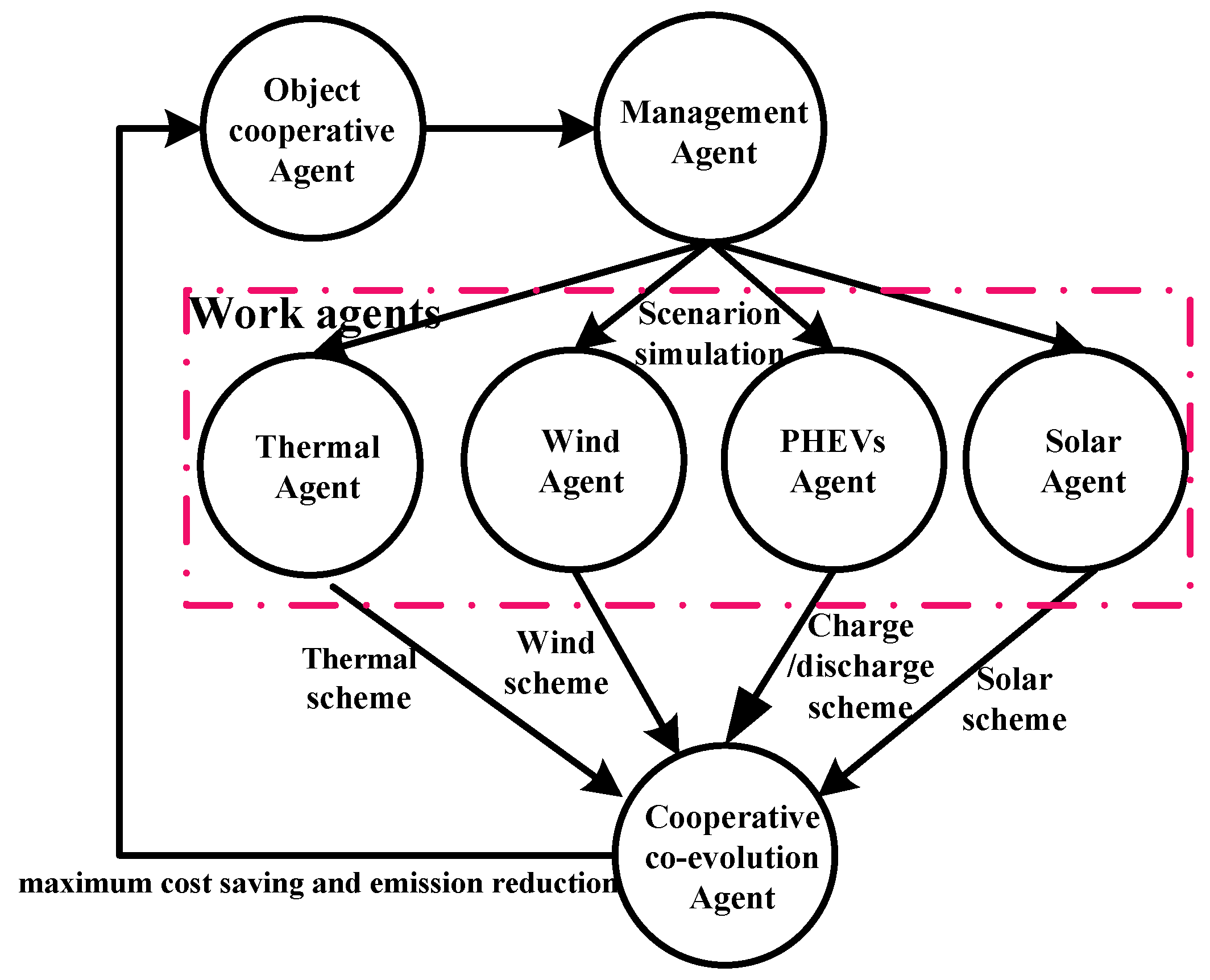
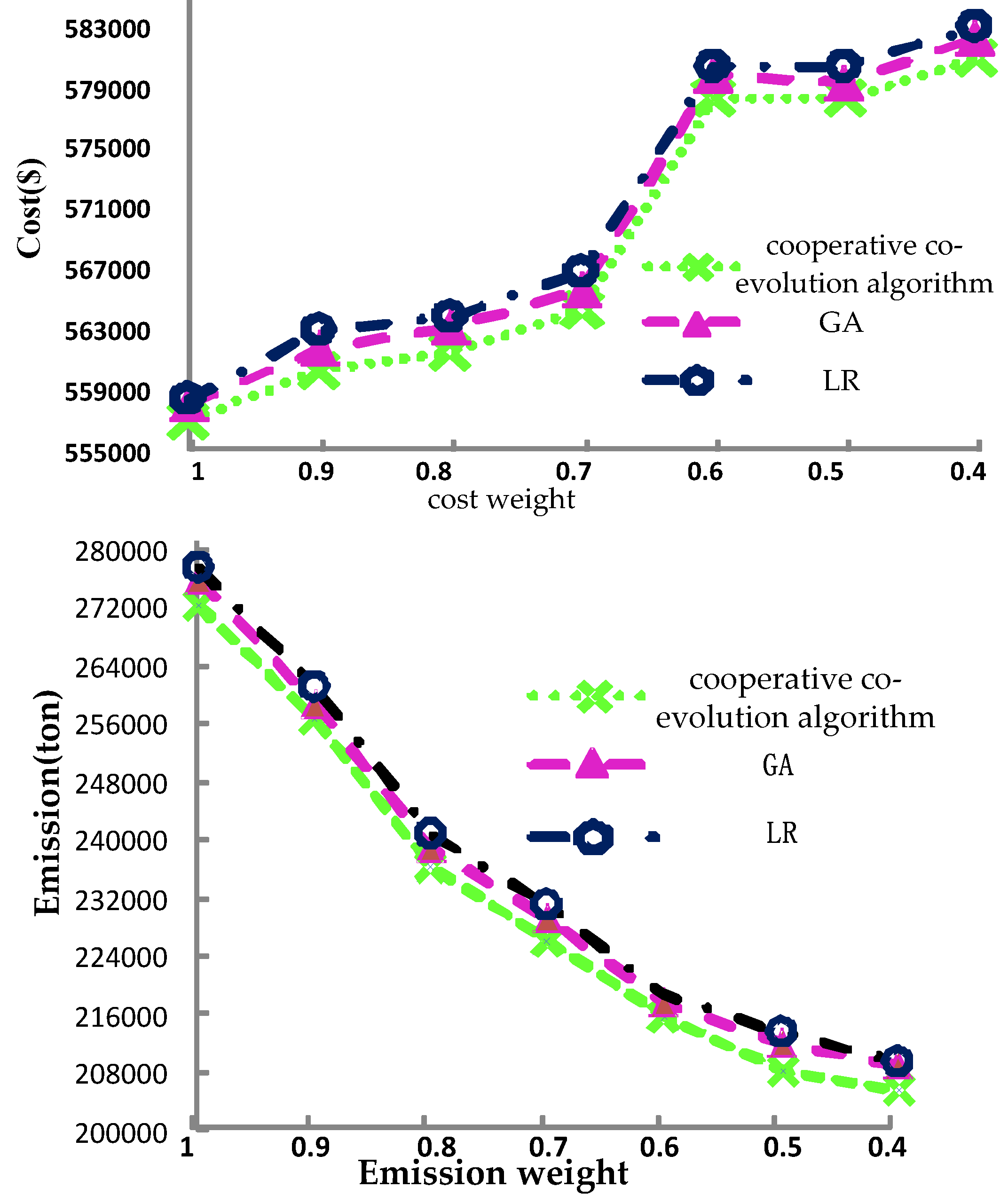
3. The Cooperative Co-Evolution Algorithm

3.1. Multi-Agent System

The MAS is a distributed computational intelligent technology, which comprises intelligent agents that work together to achieve a global goal. The key benefits of MAS are flexibility, extendibility and cooperation. Flexibility is the ability to respond to dynamic situations, extensibility is the ability to easily add new functionality and augmenting or upgrading existing functionality, and cooperation is the ability of the system to solve the problem through competition and consultation. The fundamental element of MAS is an intelligent agent [30], which is defined by some typical characteristics: reactivity, pro-activeness and social ability. Reactivity of agents is the ability to perceive their environment and respond in a timely fashion in order to satisfy their design objectives. Pro-activeness of agents exhibits goal-directed behaviors by taking the initiative in order to satisfy their design objectives. Social ability of agents is the interaction of agents with other agents in order to satisfy their design objectives. These characteristics signify the importance of MAS in developing a complex system like power distribution system. These benefits motivate the use of MAS for dispatching the smart grid with PHEVs and renewables.
In this paper, the proposed MAS for UC in smart grid consists of a thermal agent, wind agent, solar agent, PHEV agent, management agent, object cooperative agent, and a cooperative co-evolution agent. In MAS, the thermal agent, wind agent, solar agent and PHEV agent combine into work agents. Each work agent is responsible for coordinating the static scheduling of wind, solar power, TUs and PHEVs, the constraints are static for the corresponding time interval, without considering the dynamic time coupling constraints. The work agents are solved by GA with adaptive crossover and mutation operators. These agents not only have the self-target solving ability but also can achieve the common goal by their mutual cooperation. They are independent from each other. In order to achieve the system goals, the agents have to coordinate with each other through communication. Even though the goals of agents are independent, they are cooperative in the system goal optimization. The MAS of the smart grid is shown in Figure 1.
The goals of the agents are briefly provided as follows:
PHEV agent: Charge or discharge the battery in time.
Wind agent: provide power to the PHEV agent or provide power to the load based on the system condition.
Solar agent: provide power to the PHEV agent or provide power to the load based on the system condition.
Thermal agent: provide power to the PHEV agent or provide power to the load based on the system condition.
Cooperative co-evolution agent: obtain the minimum of cost and emissions for the whole scheduling cycle. The constraints are the dynamic coupling constraints on the entire scheduling period.
Object cooperative agent: control the cost and emission weight adjustment, so the trade-off can be found between cost and emissions.
Management agent: control the work agents based on the current scheduling results. After the objective cooperative agent execution, the optimization scheduling requirements are put forward to management agent. The control scheme is chosen by management agent.
Based on the MAS, the adaptive GA solves the work agents’ optimization and the cooperative multipliers are used to coordinate work agents. In this way, the cooperative co-evolution algorithm is formed.

3.2. The Adaptive Updating of Multipliers

The quality of the final optimal solution mainly depend on the cooperative multipliers. In general, adjusting cooperative multipliers by the subgradient method is hard to converge or even can’t converge in the presence of the spinning reserve constraint. In [31], the adaptive cooperative multipliers update rule is presented, showing that it is effective in improving the calculation accuracy. reduces the iteration times and saves the CPU time. In this paper, this update rule is adopted. This rule is designed so that the step size is large at the beginning of iterations and smaller as the iteration grows.
The cooperative multipliers λ t and μ t updating rule can be written as:
g λ t = { p d s t i = 1 N p i s t u i t p v N v 2 G t p p v s t p w s t   PHEVs discharging p d s t + p v N v 2 G t i = 1 N p i s t u i t p p v s t p w s t   PHEVs charging
g μ t = { p d s t + R t - i = 1 N u i t p i   max - p v m a x N v 2 G t - p w s t p p v s t   PHEVs discharging p d s t + p v m a x N v 2 G t + R t - i = 1 N u i t p i   max - p w s t p p v s t   PHEVs charging
where g λ t and g μ t are the subgradient of λ t and μ t respectively.
The corresponding norms of subgradients are as follows:
n o r m ( g λ t ) = ( g λ 1 ) 2 + ( g λ 2 ) 2 + + ( g λ T ) 2
n o r m ( g μ t ) = ( g μ 1 ) 2 + ( g μ 2 ) 2 + + ( g μ T ) 2
Each nonnegative λ t and μ t are adaptively updated by:
λ t k + 1 = max { λ t k + α k × g λ t n o r m ( g λ ) , 0 }
μ t k + 1 = max { μ t k + α k × g μ t n o r m ( g μ ) , 0 }
where k is the iteration time and α k is a scale step size.

4. Numerical Example
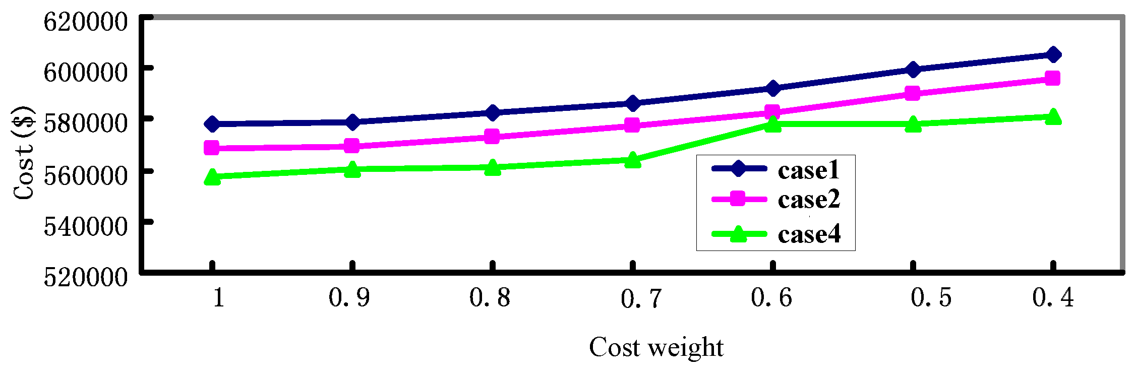
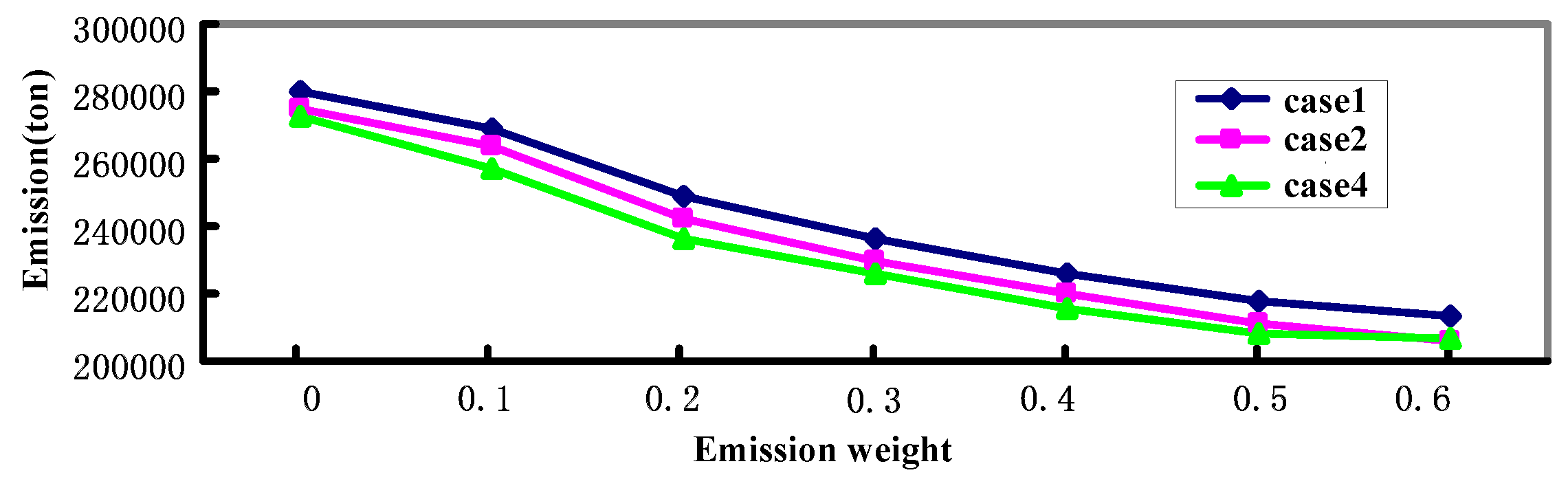
An independent system operator of a 10-unit system is considered for simulation with wind, solar power and PHEVs. The equipment cost of wind and solar powers is not taken into account. Load demand, unit characteristic and emission coefficients of the 10-unit system are collected from [2,31]. The spinning reserve is assumed to be 10% of the load demand. All PHEVs are involved in charging and discharging scheduling. The parameter values used in this paper are the same as in [2]. For practical applications, the number of PHEVs in an electric power network can be estimated analytically based on the number of electricity clients (customers) in that network. In the 10-unit system, a reasonable number of PHEVs is N v 2 G m a x = 50,000. Maximum battery capacity = 25 kWh, minimum battery capacity = 10 kWh, average battery capacity = 15 kWh, and the maximum number of charging-discharging PHEVs at each hour, N v 2 G m a x   t = 10% N v 2 G m a x . Charging and discharging frequency = one per day, scheduling period = 24 h, departure state of charging-discharging Ψ = 50%, and efficiency ξ = 85%. A PHEV needs 8.22 kWh/day, an excess of 8.22 × 50,000 = 411 MWh power is needed to run PHEVs [18]. The wind farm and solar can provide 500 MWh/day and 250 MWh/day energy, respectively. Typical day forecasts of wind and solar are given in [18].
To capture volatility, we assume the wind, solar power and load are subject to the distribution N ( μ , σ 2 ) with their expected value ( μ ) and their volatility ( σ ). In actuality, the uncertainty distribution depends on location, the nature of state variables and the forecasting/estimation tools that are used. The authors establish the discrete probabilities and expected values from their prior experience and scenario reduction technology [12].
δ w = { ( p w × 100 % , 0.5 ) ; ( p w × 99 % , 0.1 ) ; ( p w × 101 % , 0.1 ) ; ( p w × 97.5 % , 0.1 ) ; ( p w × 102.5 % , 0.1 ) ; ( p w × 95 % , 0.05 ) ; ( p w × 105 % , 0.05 ) }
δ D = { ( p d × 100 % , 0.6 ) ; ( p d × 98.5 % , 0.15 ) ; ( p d × 102 % , 0.15 ) ; ( p d × 98 % , 0.05 ) ; ( p d × 103 % , 0.05 ) }
δ p v = { ( p p v × 100 % , 0.7 ) ; ( p p v × 98.5 % , 0.1 ) ; ( p p v × 95 % , 0.05 ) ; ( p p v × 101.5 % , 0.1 ) ; ( p p v × 105 % , 0.05 ) }
where p w , p p v , p d are the predict value of wind, solar power and load.
The following four cases are presented in this study:
Case 1
the 10-unit system with standard input data of power plants, emission coefficients and load demand, considering only PHEVs.
Case 2
the 10-unit system with standard input data of power plants, emission coefficients and load demand, with wind power and PHEVs.
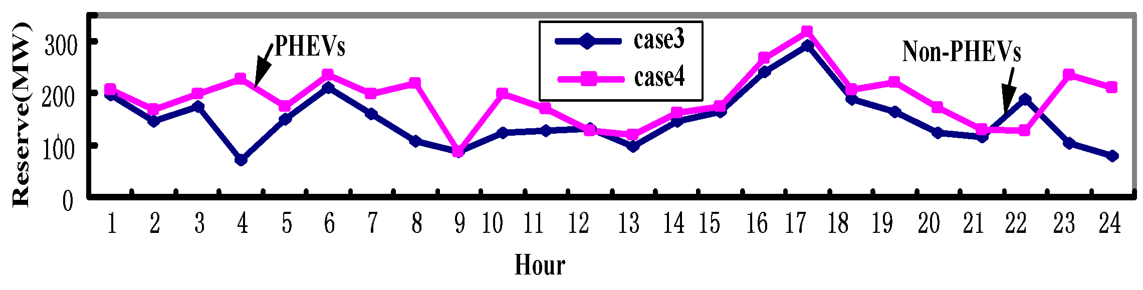
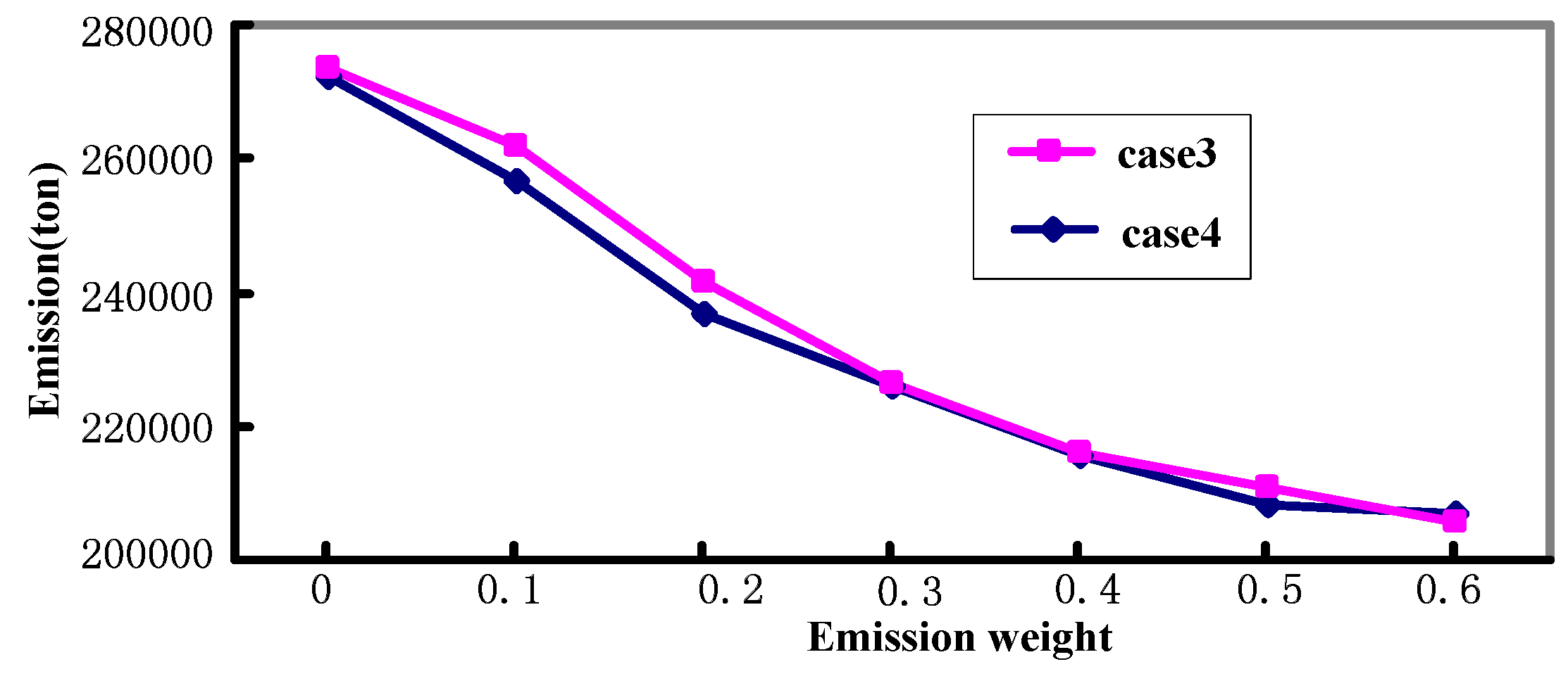
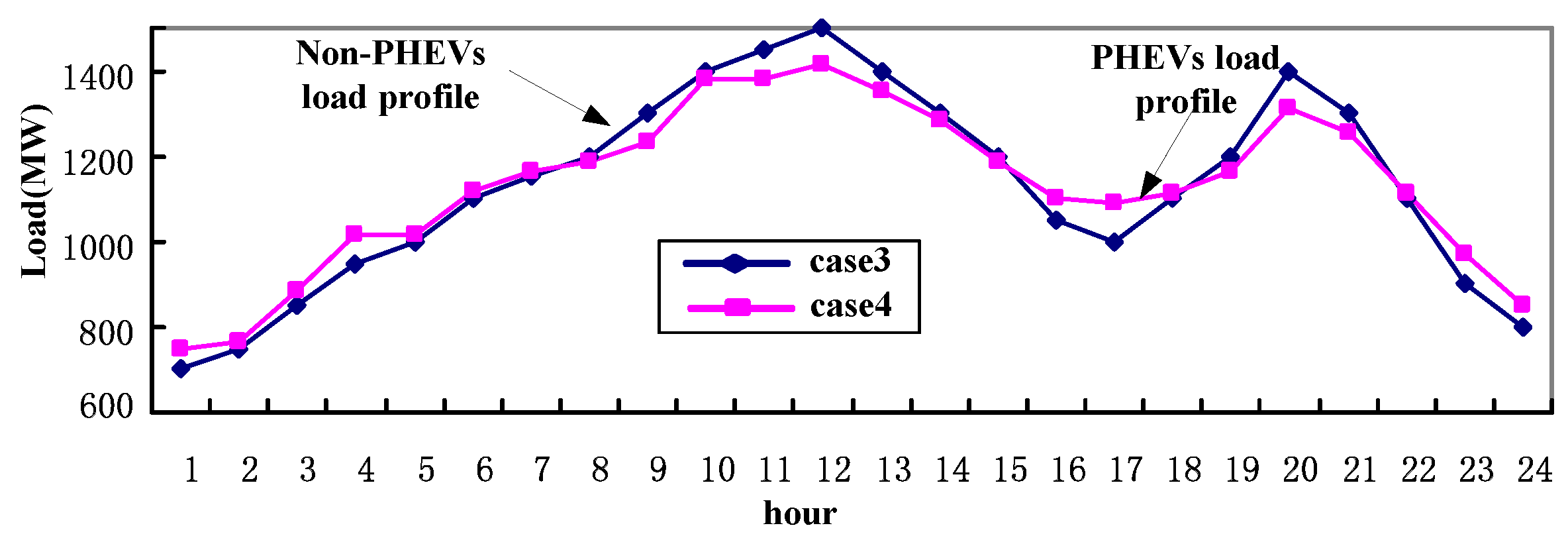
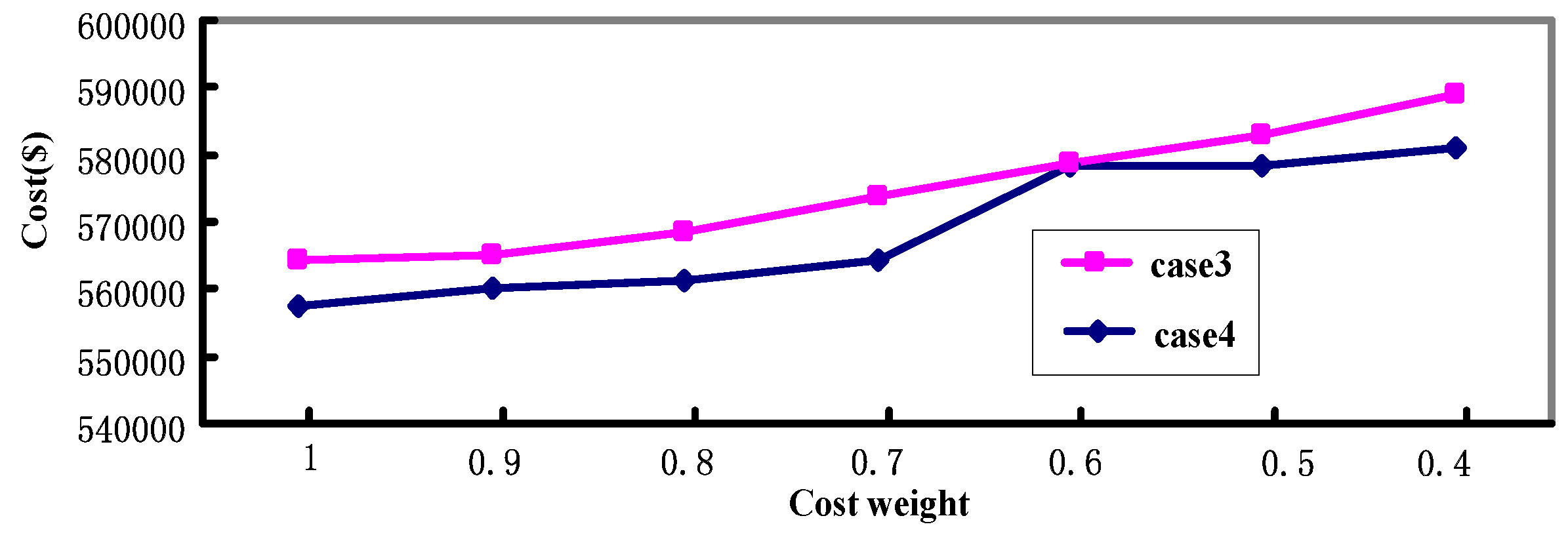
Case 3
the 10-unit system with standard input data of power plants, emission coefficients and load demand, with wind and solar power.
Case 4
the 10-unit system with standard input data of power plants, emission coefficients and load demand, considering PHEVs, wind and solar power.
These cases are studied as follows:
When cost and emission weights are (0.8, 0.2), the effect of PHEVs on the spinning reserve of smart grid with wind and solar is as shown in Figure 2. Table 1 shows the effect of PHEVs on the unit output value in smart grid with wind and solar.
Among the 24 scheduling periods, the amount of system spinning reserve is increased in Case 4 than in Case 3. In the 24 scheduling periods, the average spinning reserve is 149.2 MW in Case 3, while it is 189.5 MW in Case 4. The average spinning reserves have a surplus of 40.3 MW in Case 4 compared to Case 3.
Taking cost and emission weight (0.8, 0.2) as an example, Table 1 shows the effect of PHEVs on each unit, considering both cost and emissions. Case 4 shows the results with PHEVs, while Case 3 shows the results without PHEVs. Usually a negative effect of PHEVs indicates an expensive or more polluting unit. PHEVs reduce dependencies on small expensive units. In this instance U-1 produce same constant powers, as U-1 is the cheapest unit and it always generates maximum power; however, U-2, U-5, U-6, U-7, U-8, U-9 and U-10 generate less power when PHEVs are considered; among the ten TUs, U-7, U-8, U-9 and U-10 are expensive so they generate less power in Case 4 than in Case 3; U-2, U-5 and U-6 generate less power (negative value of V2G effect) in Case 4, because they are either (relatively) costly or more polluting units. In this instance U-3 and U-4 generate more power (positive value of PHEVs effect) in Case 6, because the proposed method makes a balance between the cost and emissions, and it satisfies all the constraints of the system.
Figure 3 shows the influence of PHEVs on load curve. Figure 4 and Figure 5 are the system costs and emissions with PHEVs in different cases; Figure 6 and Figure 7 are the influence of PHEVs on cost and emissions in cases 3 and 4.
The load curve of the 10-unit system with wind and solar power has both peaks and valleys. According to the load curve, demand is relatively low during the hours from 1st to 7th, from 16th to 18th and from 22nd to 24th; demand is relatively high during the hours from 8th to 15th and from 19th to 21st. PHEVs can be charged from the grid during the off-peak load to level the demand, it can be discharged from the grid during the peak load. They maximize renewable energy use for charging, and when it is not enough, using low cost and pollutant units’ power for charging. In the proposed method, an extra 411 MWh load for 50,000 PHEVs is intelligently distributed among off-peak hours, while these PHEVs smartly discharge among peak hours so that cost and emissions are minimized. From Figure 3, the difference between peak and valley changes from 800 MW (in case 3) to 666.5 MW (in case 4), a reduction of 133.5 MW. By intelligent charging and discharging control of PHEVs in the smart grid, load leveling is better than typical static load leveling. It reduces the system dependence on high cost, high emissions units, enhancing the ability of energy-saving emission reduction.
From Figure 4 and Figure 5, emissions are always high when cost is mainly considered in the model to generate a low cost schedule. On the other hand, emissions are always low and cost is very high when emissions are mainly considered in the model to generate an environmental friendly schedule. With the same cost and emissions weights, among the three cases, the operation cost in Case 4 is the lowest, in Case 1 is the highest, and in Case 2 is the middle. When the system operation cost is the highest, the corresponding emissions are the greatest. Taking the cost and emissions weight (0.8, 0.2) as an example, the operation cost is $582,329.6 and the emissions are 248,920.4 t in Case 1; the operation cost is $573,136.8 and the emissions are 242,164.4 t in Case 2; the operation cost is $561,436.6 and the emissions are 236,585.4 t in Case 4. The cost is reduced by $20,893 ($582,329.6 − $561,436.6) and the total emission is reduced by 12,335 t (248,920.4 − 236,585.4 t). According to Figure 4 and Figure 5, with the reduction of W c , W e increases, the operation cost increases, while the emission reduces. For practical use, values of W c and W e should be chosen carefully considering price, environment effects, consumers’ and system operators’ demand. So the trade-off can be found between cost and emissions in this paper.
Similarly Figure 6 and Figure 7 show the cost and emissions with and without PHEVs in different weights. From Figure 6 and Figure 7, taking the cost and emissions weight (0.8, 0.2) as an example, the operation cost is $568,568.5 and the emissions are 241,552.8 t in Case 3; the operation cost is $561,436.6 and the emissions are 236,585.4 t in Case 4. Total emissions are reduced by 4967.4 t (241,552.8 − 236,585.4 t) per day and cost is reduced by $7,131.9 ($568,568.5 − $561,436.6) per day. By PHEVs’ intelligent charging and discharging control, the system’s dependency on small expensive and pollutant units in peak hours is reduced. In this way, PHEVs help to reduce both cost and emissions in power systems (Figure 6 and Figure 7). Therefore intelligent UC with PHEVs, for both cost and emission optimization, is essential in power systems.
The proposed cooperative co-evolution algorithm is compared with GA [32] and conventional Lagrangian relaxation (LR) [33] as illustrated in Figure 8.
As shown in Figure 8, the costs and emissions of the proposed cooperative co-evolution algorithm are shown to be less than those of GA [32], LR [33] in Case 4 with the same weights. Taking the cost and emissions weight (0.8, 0.2) as an example, the findings are as follows: (1) the operation cost and the emissions of GA are $563,186.5 and 239,064.2 t, respectively; (2) the operation cost and the emissions of LR are $563,815.4 and 240,854.4 t, respectively; (3) the operation cost and the emissions of the proposed cooperative co-evolution algorithm are $561,436.6 and 236,585.4 t, respectively. Among the three methods, the operation cost and emissions under the proposed cooperative co-evolution algorithm are the lowest. Total emissions are reduced by 4269 t (240,854.4 − 236,585.4 t) per day and while total costs are reduced by $2,378.8 ($563,815.4 − $561,436.6) per day.
Similarly Table 2 shows the effects of cooperative multipliers updating methods on the smart grid.
Taking the cost and emission weight (0.8, 0.2) as an example, the cooperative multipliers updating method in Case 4 is analyzed. In order to obtain the optimal solution, the operation time is 132 s by adaptive cooperative multipliers updating method, while the subgradient method is 250 s. The operation cost and emissions by adaptive cooperative multipliers updating method are $561,436.6 and 236,585.4 t, and by the subgradient method are $567,255.4 and 239,786.5 t. The adaptive cooperative multipliers updating method not only can improve quality of the solutions but can save computing time.

5. Conclusions

The co-evolutionary agents in MAS are employed for a smart grid UC with the randomness of wind and solar power, and the intelligent charging and discharging control of PHEVs, with consideration of the system energy saving and emissions reduction. In the sustainable smart grid, cooperative utilization of wind and solar power is effective to reduce cost and emissions. The amount of cost and emissions reductions mainly depends on maximum utilization of renewable energy through PHEVs. Compared with GA and conventional LR, the operation cost and emissions under the proposed cooperative co-evolution algorithm are the lowest. The proposed adaptive multipliers updating strategy can save computation time and improve operation efficiency. By the reasonable selection of cost and emission weights, it can realize an effective compromise between energy saving and emissions reduction.

Acknowledgments

This work is supported by Jiangsu Natural Science Foundation (Grant No.bk20140265) Cooperative Innovation Fund of Industry, Education and Academy of Jiangsu Province (Grant No. BY2014037-29), Jiangsu province science and technology support program (industry) project (BE-2013005-3) and Jiangsu Key Laboratory of Power Transmission and Distribution Equipment Technology project (2011JSSPD10).

Author Contributions

All the authors contributed to this work. Xiaohua zhang designed the study, developed the mathematical model, performed the analysis and checked the overall logic of this work. Jun Xie developed stochastic cost-emission reduction model and multi-agent system. Zhengwei Zhu contributed to the conceptual approach and provided important comments on the modeling and analysis. Jianfeng Zheng contributed towards the optimization algorithm. Hao Qiang and Hailong Rong contributed towards seting the simulation environment and performing the simulations.

Conflicts of Interest

The authors declare no conflict of interest.

References

  1. Moreno, J.; Ortzar, M.E.; Dixon, J.W. Energy-management system for a hybrid electric vehicle, using ultra capacitors and neural networks. IEEE Trans. Ind. Electron. 2006, 53, 614–623. [Google Scholar] [CrossRef]
  2. Saber, A.Y.; Venayagamoorthy, G.K. Intelligent unit commitment with vehicle-to-grid-A cost-emission optimization. J. Power Sources 2010, 195, 898–911. [Google Scholar] [CrossRef]
  3. Hadley, S.W.; Tsvetkova, A. Potential Impacts of Plug-in Hybrid Electric Vehicles on Regional Power Generation; Oak Ridge National Laboratory: Oak Ridge, TN, USA, January 2008. [Google Scholar]
  4. Sioshansi, R.; Fagiani, R.; Marano, V. Cost and emissions impacts of plug-in hybrid vehicles on the Ohio power system. Energy Policy 2010, 38, 6703–6712. [Google Scholar] [CrossRef]
  5. Huber, M.; Trippe, A.; Kuhn, P.; Hamacher, T. Effects of large scale EV and PV integration on power supply systems. In Proceedings of the IEEE PES Innovative Smart Grid Technologies Conference Europe, European, Berlin, Germany, 14–17 October 2012; pp. 1–8.
  6. Wang, J.; Liu, C.; Ton, D.; Zhou, Y.; Kim, J.; Vyas, A. Impact of plug in hybrid electric vehicles on power systems with demand response and wind power. Energy Policy 2011, 39, 1–6. [Google Scholar] [CrossRef]
  7. Haque, A.; Mandal, P.; Meng, J.; Negnevitsky, M. Wind speed forecast model for wind farm based on a hybrid machine learning algorithm. Int. J. Sustain. Energy 2015, 34, 38–51. [Google Scholar] [CrossRef]
  8. Mandal, P.; Zareipour, H.; Rosehart, W.D. Forecasting aggregated wind power production of multiple wind farms using hybrid wavelet-PSO-NNs. Int. J. Energy Res. 2014, 38, 1654–1666. [Google Scholar] [CrossRef]
  9. Haque, A.; Mandal, P.; Nehrir, M.H. A hybrid intelligent model for deterministic and quantile regression approach for probabilistic wind power forecasting. IEEE Trans. Power Syst. 2014, 29, 1663–1672. [Google Scholar] [CrossRef]
  10. Haque, A.; Mandal, P.; Meng, J.; Tseng, T.-L.; Senjyu, T. A novel hybrid approach based on wavelet transform and fuzzy ARTMAP network for predicting wind farm power production. IEEE Trans. Ind. Appl. 2013, 49, 2253–2261. [Google Scholar] [CrossRef]
  11. AlHakeem, D.; Mandal, P.; Haque, A.; Yona, A.; Senjyu, T.; Tseng, T.-L. A new strategy to quantify uncertainties of Wavelet-GRNN-PSO based solar PV power forecasts using bootstrap confidence intervals. In Proceedings of the IEEE Power & Energy Society General Meeting, Denver, CO, USA, 26–30 July 2015.
  12. Wang, J.; Shahidehpour, M.; Li, Z. Security constrained unit commitment with volatile wind power generation. IEEE Trans. Power Syst. 2008, 23, 1319–1327. [Google Scholar] [CrossRef]
  13. Swider, D.J.; Weber, C. The costs of wind intermittency in Germany: Application of a stochastic electricity market model. Eur. Trans. Electr. Power 2007, 17, 151–172. [Google Scholar] [CrossRef]
  14. Hargreaves, J.J.; Hobbs, B.F. Commitment and dispatch with uncertain wind generation by dynamic programming. IEEE Trans. Sustain. Energy 2012, 3, 724–734. [Google Scholar] [CrossRef]
  15. Chakraborty, S.; Ito, T.; Senjyu, T.; Saber, A.Y. Intelligent economic operation of smart-grid facilitating fuzzy advanced quantum evolutionary method. IEEE Trans. Sustain. Energy 2013, 4, 905–916. [Google Scholar] [CrossRef]
  16. Tuohy, A.; Meibom, P.; Denny, E.; O’Malley, M. Unit commitment for systems with significant wind penetration. IEEE Trans. Power Syst. 2009, 24, 592–601. [Google Scholar] [CrossRef] [Green Version]
  17. Wind Power Integration in Liberalised Electricity Markets (Wilmar) Project. Available online: http://www.wilmar.risoe.dk (accessed on 1 December 2003).
  18. Ahmed, Y.S.; Venayagamoorthy, G.K. Resource scheduling under uncertainty in a smart grid with renewables and plug-in vehicles. IEEE Syst. J. 2012, 6, 103–109. [Google Scholar]
  19. Sheble, G.B. Solution of the unit commitment problem by the method of unit periods. IEEE Trans. Power Syst. 1990, 5, 257–260. [Google Scholar] [CrossRef]
  20. Ouyang, Z.; Shahidehpour, S.M. An intelligent dynamic programming for unit commitment application. IEEE Trans. Power Syst. 1991, 6, 1203–1209. [Google Scholar] [CrossRef]
  21. Snyder, W.L., Jr.; Powell, H.D., Jr.; Rayburn, J.C. Dynamic programming approach to unit commitment. IEEE Trans. Power Appl. Syst. 1987, 2, 339–348. [Google Scholar] [CrossRef]
  22. Simoglou, C.K.; Biskas, P.N.; Bakirtzis, A.G. Optimal self-scheduling of a thermal producer in short-term electricity markets by MILP. IEEE Trans. Power Syst. 2010, 25, 1965–1977. [Google Scholar] [CrossRef]
  23. Cohen, A.I.; Yoshimura, M. A branch-and-bound algorithm for unit commitment. IEEE Trans. Power Appl. Syst. 1983, 2, 444–451. [Google Scholar] [CrossRef]
  24. Dang, C.Y.; Li, M.Q. Floating-point genetic algorithm for solving the unit commitment problem. Eur. J. Oper. Res. 2007, 181, 1370–1395. [Google Scholar] [CrossRef]
  25. Swarup, K.S.; Yamashiro, S. Unit commitment solution methodology using genetic algorithm. IEEE Trans. Power Syst. 2002, 17, 87–91. [Google Scholar] [CrossRef]
  26. Ouyang, Z.; Shahidehpour, S.M. A hybrid artificial neural network-dynamic programming approach to unit commitment. IEEE Trans Power Syst. 1992, 7, 236–242. [Google Scholar] [CrossRef]
  27. Logenthiran, T.; Srinivasan, D. Multi-agent system for managing a power distribution system with plug-in hybrid electrical vehicles in smart grid. In Proceedings of the IEEE PES Innovative Smart Grid Technologies, Kerala, India, 1–3 December 2011; pp. 346–351.
  28. Gallehdari, Z.; Meskin, N.; Khorasani, K. Cost performance based control reconfiguration in multi-agent systems. In Proceedings of the American Control Conference, Portland, OR, USA, 4–6 June 2014; pp. 509–516.
  29. Goh, C.K.; Tan, K.C. A competitive-cooperative coevolutionary paradigm for dynamic multiobjective optimization. IEEE Trans. Evolut. Comput. 2009, 13, 103–127. [Google Scholar]
  30. Shao, S.; Pipattanasomporn, M.; Rahman, S. Challenges of phev penetration to the residential distribution network. In Proceedings of the IEEE PES General Meeting, Calgary, AB, Canada, 26–30 July 2009; pp. 1–8.
  31. Ongsaku, W.; Petcharaks, N. Unit commitment by enhanced adaptive lagrangian relaxation. IEEE Trans. Power Syst. 2004, 19, 620–628. [Google Scholar] [CrossRef]
  32. Sun, L.Y.; Zhang, Y.; Jiang, C.W. A matrix real-coded genetic algorithm to the unit commitment problem. Electr. Power Syst. Res. 2006, 76, 716–728. [Google Scholar] [CrossRef]
  33. Kazarlis, S.A.; Bakirtzis, A.G.; Petridis, V. A genetic algorithm solution to the unit commitment problem. IEEE Trans. Power Syst. 1996, 11, 83–92. [Google Scholar] [CrossRef]
Figure 1. Multi-agent scheduling system based on a smart grid.
Energies 09 00834 g001
Figure 2. The effect of plug-in hybrid electric vehicles (PHEVs) on the spinning reserve of a smart grid.
Energies 09 00834 g002
Figure 3. The influence of PHEVs on load curve in smart grid.
Energies 09 00834 g003
Figure 4. The operation cost with PHEVs in different cases.
Energies 09 00834 g004
Figure 5. The emission with PHEVs in different cases.
Energies 09 00834 g005
Figure 6. The influence of PHEVs on operation cost in smart grid.
Energies 09 00834 g006
Figure 7. The influence of PHEVs on emission in smart grid.
Energies 09 00834 g007
Figure 8. The comparison of cost and emission in different methods in Case 4.
Energies 09 00834 g008
Table 1. Power from generating units during 24 h considering PHEVs.
Unit Output (MW)U-1U-2U-3U-4U-5U-6U-7U-8U-9U-10
Case 4 (MW)10,9208034.3260028602222.7410.510020100
Case 3 (MW)10,9208130.3234027302275.5544.612562.13020
PHEVs Effect (MW)0−96260130−52.8−134.1−25−42.1−20−20
Table 2. The effects of coordinating multipliers updating method on smart grid.
Cooperative Multiplier Updating MethodsSubgradientAdaptive
Cost ($)567,255.4561,436.6
Emissions (t)239,786.5236,585.4
Operation time (s)250132

