Numerical Study on Self-Starting Performance of Darrieus Vertical Axis Turbine for Tidal Stream Energy Conversion

Abstract

Self-starting performance is a key factor in the evaluation of a Darrieus straight-bladed vertical axis turbine. Most traditional studies have analyzed the turbine’s self-starting capability using the experimental and numerical data of the forced rotation. A 2D numerical model based on the computational fluid dynamics (CFD) software ANSYS-Fluent was developed to simulate the self-starting process of the rotor at constant incident water-flow velocities. The vertical-axis turbine (VAT) rotor is driven directly by the resultant torque generated by the water flow and system loads, including the friction and reverse loads of the generator. It is found that the incident flow velocity and the moment of inertia of the rotor have little effect on the averaged values of tip-speed ratios in the equilibrium stage under no-load conditions. In the system load calculations, four modes of the self-starting were found: stable equilibrium mode, unstable equilibrium mode, switch mode and halt mode. The dimensionless power coefficient in the simulations of passive rotation conditions is found to be, on average, 38% higher than those achieved in the simulations of forced rotation conditions.

1. Introduction

Abundant resources of marine energy make it possible to use the energy in the ocean as an alternative and renewable power source in the future. However, harvesting the marine energy has been a big challenge to the ocean engineers. The tidal stream energy has advantages such as stable energy flux density and high predictability. The devices to capture the tidal stream energy always borrow the idea from the wind energy turbine because of the similarity of these two working fluids. Compared to the more common horizontal-axis turbine, the vertical-axis turbine (VAT) is more adaptable to the direction change of tidal currents. The VAT is also easier to access for maintenance because the electrical generators in the VAT are always installed near or above the water surface.

The Darrieus straight-bladed turbine is a typical VAT; it is widely employed for wind and tidal stream energy conversion. The VAT typically suffers from a serious drawback: the blades are stalled or show a poor performance at a low tip-speed-ratio (TSR) owing to the low or even negative (reverse) torque for most azimuth angles [1]. Therefore, the Darrieus turbine was regarded by some scholars to be inherently non self-starting, which can be fixed by utilizing the variable-pitched blades [2,3]. Although the exact definition of self-starting is not consistent throughout the literature, the self-starting performance of the Darrieus VAT has been a main research topic, especially for the small and standalone cases in the field of wind energy [4].

The inability of a Darrieus turbine of low solidity to self-start arises from the existence of a band of TSRs below the operating condition during which the net amount of energy collected by each blade in one revolution is negative [5]. This negative or reverse torque region is called the “dead band”; this was plotted as C_p (dimensionless power coefficient)—λ (TSR) curves in [6]. The corresponding analytical investigations were based on the experimental results of the aerodynamic performance of airfoils [7]. It was reported that the VAT has the lowest self-starting capability with NACA 0012 [8] and a highest capability with NACA 0021, among the various symmetric airfoils investigated [9]. Different blade geometries have been proposed and tested to improve the self-starting capability of the VAT [10,11,12,13,14,15,16]. The blade pitch control was also found to be an effective method for the VAT to have a better self-starting capability [17,18]. External auxiliaries, such as the combined Savonius turbine [19] and the ailerons [20], were proposed to improve the self-starting performance of the Darrieus straight-bladed VAT. It was pointed out that inaccurate modeling of the dead band may result in a false prediction due to the effects of dynamic stall and wake interaction being neglected [21].

Therefore, besides experimental studies in the wind tunnel, the computational fluid dynamics (CFD) approach was adopted for the investigations on the self-starting of direct-driven turbine. These studies can reveal the starting characteristics and the related flow fields of a VAT from rest till the operational rotating speed is reached [22,23,24,25]. The CFD approach was also adopted in the studies on the self-starting of VATs for tidal stream energy conversion [26,27].

In this study, the definition of self-starting for the Darrieus turbine is introduced in Section 2. In Section 3, a 2D numerical model based on the CFD software ANSYS-Fluent (Canonsburg, PA, USA) is presented and validated. The flow-driven passive rotations of the 2D rotor are simulated numerically. In Section 4, the variations in the flow fields, rotor torques and dimensionless power coefficients are also analyzed. The effects of incident flow velocities, load conditions and moments of inertia on the self-starting characteristics of the VAT are studied. Four self-starting modes of the Darrieus VAT are considered. The main conclusions derived from the results of the 2D numerical simulations and the proposed future work are discussed in Section 5.

2. Self-Starting of Darrieus VAT

A Darrieus straight-bladed VAT was employed in this study. The shape of the cross section of the blade is as per the NACA 0018 airfoil. The blade span is taken as 1 m in the 2D calculations of ANSYS-Fluent. The parameters of the turbine rotor are shown in

Table 1. Shape parameters of the vertical-axis turbine (VAT) rotor.

Description	Value
Number of blades N	3
Blade chord C (m)	0.12
Blade span S (m)	1.0
Radius of rotor R (m)	0.5
Solidity σ	0.36
Fixed pitch angle β	0°

. The solidity of the rotor is calculated using the equation σ = N·C/2R.

One definition of self-starting, given in [6], is that the turbine is considered as self-starting if it can accelerate from rest to the point where a significant power is produced. However, the term “significant power” has not been defined precisely. Another specific definition is that the turbine is deemed to have started if it has accelerated from rest to a condition where the blade operates at a steady speed that exceeds the fluid speed (TSR > 1) [21]. Both of these simple definitions of self-starting, in terms of the load or the TSR, have their drawbacks [28].

The term “self-starting” mentioned in [28] refers to the ability to accelerate from rest to the final operating TSR. For a given VAT rotor, the final operating TSR depends on the incident flow conditions and the load conditions. As pointed out in [29], the final TSR increases with an increase of the incident free velocity and a decrease of the resistive load, and vice versa. If the resistive load is very high, the turbine will fall into the dead band. Based on this information, the turbine can be deemed to be “self-starting” if it meets the following conditions: “The turbine can accelerate from rest to a final tip-speed-ratio to deliver a continuous thrust output, which is an equilibrium point where the fluid dynamic and resistive torques match [29]”.

The TSR is defined as:

$$\lambda =\frac{\omega \cdot R}{U_{\infty }}$$

(1)

where ω is the angular velocity of the rotor and U_∞ is the free water flow from the far field.

The dimensionless power coefficient C_p can be defined as:

$$C_p=\frac{\omega \cdot T_q}{0.5\rho U_{\infty }^3{A}_r}$$

(2)

where T_q is the instantaneous torque generated by the turbine, and ρ is the density of water. A_r is the swept area, which can be calculated as: A_r = 2R·S.

The averaged dimensionless power coefficient C_p-ave in a revolution is defined as:

$$C_{p-ave}=\frac{1}{T}{\displaystyle \underset{t}{\overset{t+T}{\int }}{C}_{p}dt}$$

(3)

where T is the period of revolution.

3. Numerical Model

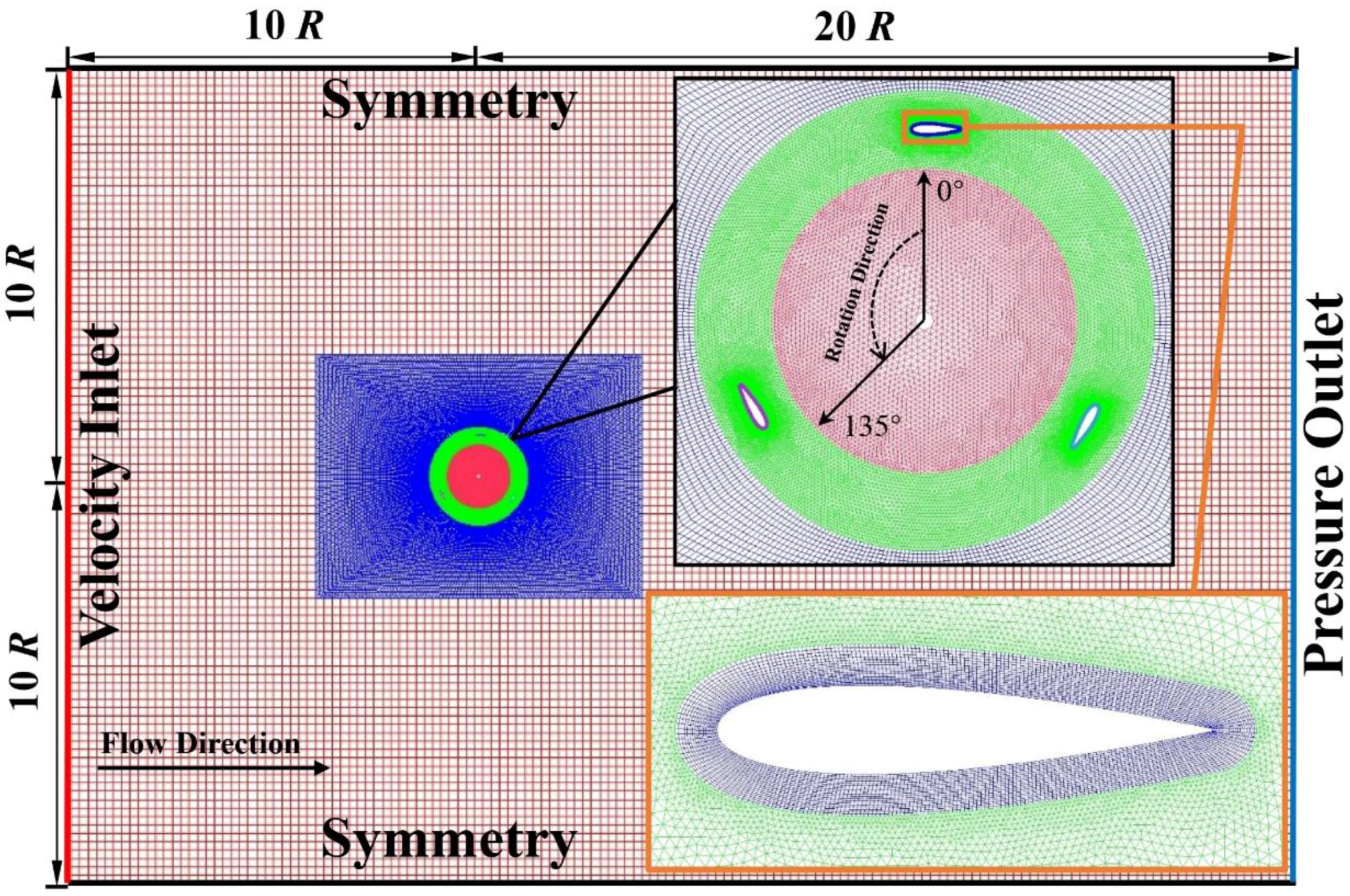
3.1. Numerical Set-up

Although the 2D CFD model cannot reflect all the hydrodynamic characteristics of the VAT and will ignore some parasitic drag forces [30], it has been pointed out that the 2D model is suitable for the initial study to save computational cost and time [23]. Considering that the numerical simulation of the self-starting of a VAT is still in a preliminary stage, we decided to use the 2D model in this study. The continuity equation of incompressible fluids and unsteady Reynolds-averaged Navier–Stokes equations are applied as the governing equations. These equations are solved in the general-purpose commercial CFD platform ANSYS-Fluent 12.0. The finite volume method is used for discretization using the pressure-based solver. Spatial and temporal discretizations of second order were used for all the equations and the SIMPLE (Semi-Implicit Method for Pressure Linked Equations) scheme for the solution of the governing equations.

The rectangular computational domain is shown in Figure 1. The length and width of the domain are 30 times and 20 times the rotor radius, respectively. The left and right sides are set as the boundaries of the velocity inlet and pressure outlet, respectively. The other two sides are set as symmetry boundaries. The rotor is placed at a distance of 10R from the velocity inlet to ensure the full development of the incident flow from the far field and wake formation in the downstream. The core domain is at a distance of 10R from both the symmetry boundaries to reduce the sidewall effects as much as possible. The incident flow direction and the azimuth angle of 0° are also defined in Figure 1.

The computational domain is divided into three parts: the circular-ring rotational domain and the outer and inner stationary sub-domains. The circular ring domain (green part) can rotate together with three blades, and a sliding mesh model is coupled with this domain. The stationary and rotational sub-domains are connected to each other through non-conformal interfaces. The mesh motions are prescribed so that the sub-domains linked at the interfaces can remain in contact with each other (sliding along the interface boundaries) to ensure an accurate exchange of all the flux at the interfaces and a faster computational convergence.

To reduce the computation time by accelerating the iteration speeds and to improve the precision in calculation with respect to the reduction of possible errors, as many structured meshes as possible are used in the outside domain. The rotational and inner stationary sub-domains are meshed with unstructured elements to fit the complex geometries. The boundary layer meshes around the blade foils are refined to capture the near-wall turbulence effects and the wake formations. The wall y+ is controlled to be from 20 to 60. The shear stress transportation (SST) turbulence model with approximately 2 × 10⁵ meshes and a time step of 0.005 s is employed in this study; this has been investigated and validated in a previous study by the authors [31].

The description of the flow-driven passive rotation of the VAT rotor is based on Newton’s second law, which can be defined as:

$$I\cdot \frac{d\omega }{dt}+T_s=T_w$$

(4)

where I is the moment of inertia of the rotor, and T_w is the hydrodynamic torque generated by the incident water flow. T_S is the system load, which consists of the friction load T_f and the resistive load of the electric generator T_g. The friction load is kept constant. For a permanent magnetic synchronous generator (PMSG), T_g can be simplified as:

$$T_g=\{\begin{array}{cc}\hfill T_I\hfill & Whentherotorisatrest;\hfill \\ \hfill k\cdot \omega \hfill & Whentherotorisrotating.\hfill \end{array}$$

(5)

where T_I is the initial resistive torque of the generator, and k is a constant-ratio, whose unit is N·ms/rad.

From Equation (4), at the time of t + ∆t, the rotation speed of the rotor can be calculated using the following equation:

$${\omega }_{t+\Delta t}={\omega }_t+\frac{\left(T_w-T_s\right){|}_t}{I}\Delta t$$

(6)

Furthermore, the instantaneous azimuth angle θ_t+∆t at the same time is updated as:

$${\theta }_{t+\Delta t}={\theta }_t+{\omega }_{t+\Delta t}\cdot \Delta t$$

(7)

where θ_t is the azimuth angle at the time of t.

The new positions of the blades are derived from Equation (7), and cause the flow fields around the rotor to be updated. After this step, the torque of the rotor at the new azimuth is then renewed. The coupling of the fluid-structure interaction in Fluent is achieved through a user-defined function (UDF). The torque of the rotor is calculated by the integration of the pressures on each grid of the blade surface. By executing the above loop, the passive rotation of the VAT rotor, including the fluid-structure interaction, can be obtained.

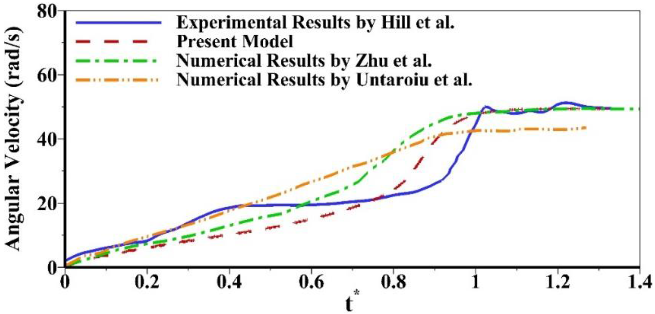
3.2. Experimental Validation

To validate the capability of the above numerical model, in order to predict the fully passive self-starting performance, the experimental results of the Darrieus straight-bladed VAT rotor should be used for comparison. However, valuable experimental data pertaining to the self-starting of the tidal turbine were not available during literature review. Therefore, the results of experiments conducted on a prototype wind turbine, reported by Hill et al. [7], were used. The blade profile used in the experiments was that of the NACA 0018 airfoil and the blade span was 0.6 m and the free wind speed was 6 m/s. A comparison of the experimental and numerical results is shown in Figure 2.

In Figure 2, the dimensionless time t* is defined as t* = t/t_s, where t_s is the time when a steady rotation speed is achieved. It can be seen that the self-starting process can be divided into three stages: the linear acceleration, plateau and equilibrium stages. Untaroiu et al. successfully predicted the linear acceleration stage and the angular velocity increased linearly before reaching the equilibrium stage [22]. However, the final steady angular velocity was underestimated. The present model shows performance similar to that obtained using the numerical model established by Zhu et al. [24]. The linear acceleration stage was underestimated, but the equilibrium stage was well predicted. Compared to the previous model, the numerical model in this study yields a closer prediction of the acceleration stage connecting the plateau and equilibrium stages. Moreover, the present model predicts the value of final steady rotational speed precisely.

In addition, t_s in the experiment is around 154 s. The values of t_s calculated in the grid independence study by Zhu et al. [24] are from 8 s to 15 s, which are approximately ten times smaller than that of experimental result. Untaroiu et al. gave a better prediction on t_s in the 3D model, which is around 150 s [22]. The steady angular velocity predicted by using the present model is achieved a little faster than the experiments, and t_s is around 134 s. The inaccurate predictions of angular velocities in the plateau stage and the value of t_s may be because of the finite blade height and the drags created by the spokes. Except the time when the steady rotation speed is achieved, the present numerical model shows a better capability to predict the entire self-starting process than the other numerical models. The comparison indicates that the passive rotation model used in this study can capture the main features of the angular velocity during self-starting under the uniform flow conditions.

4. Results and Discussion

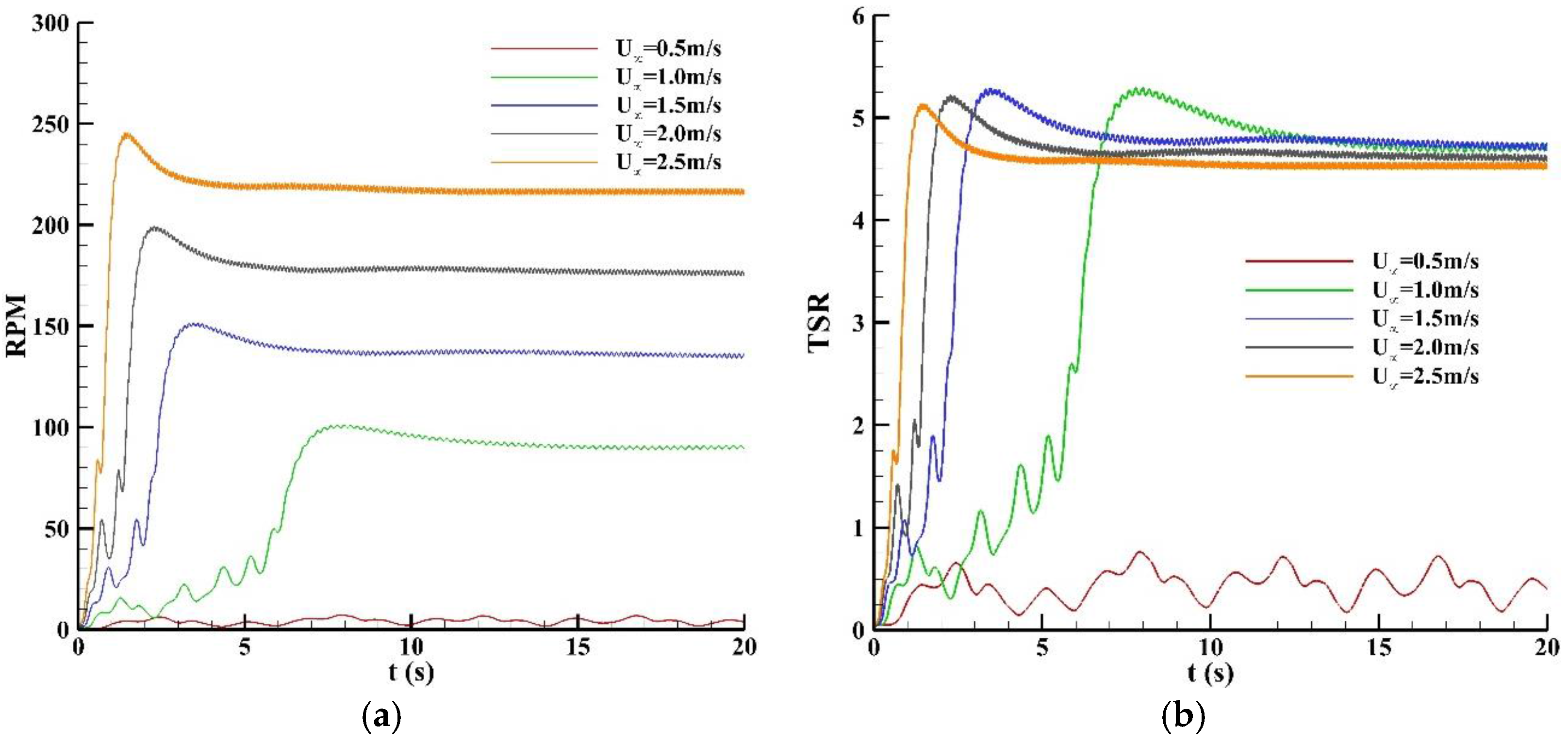
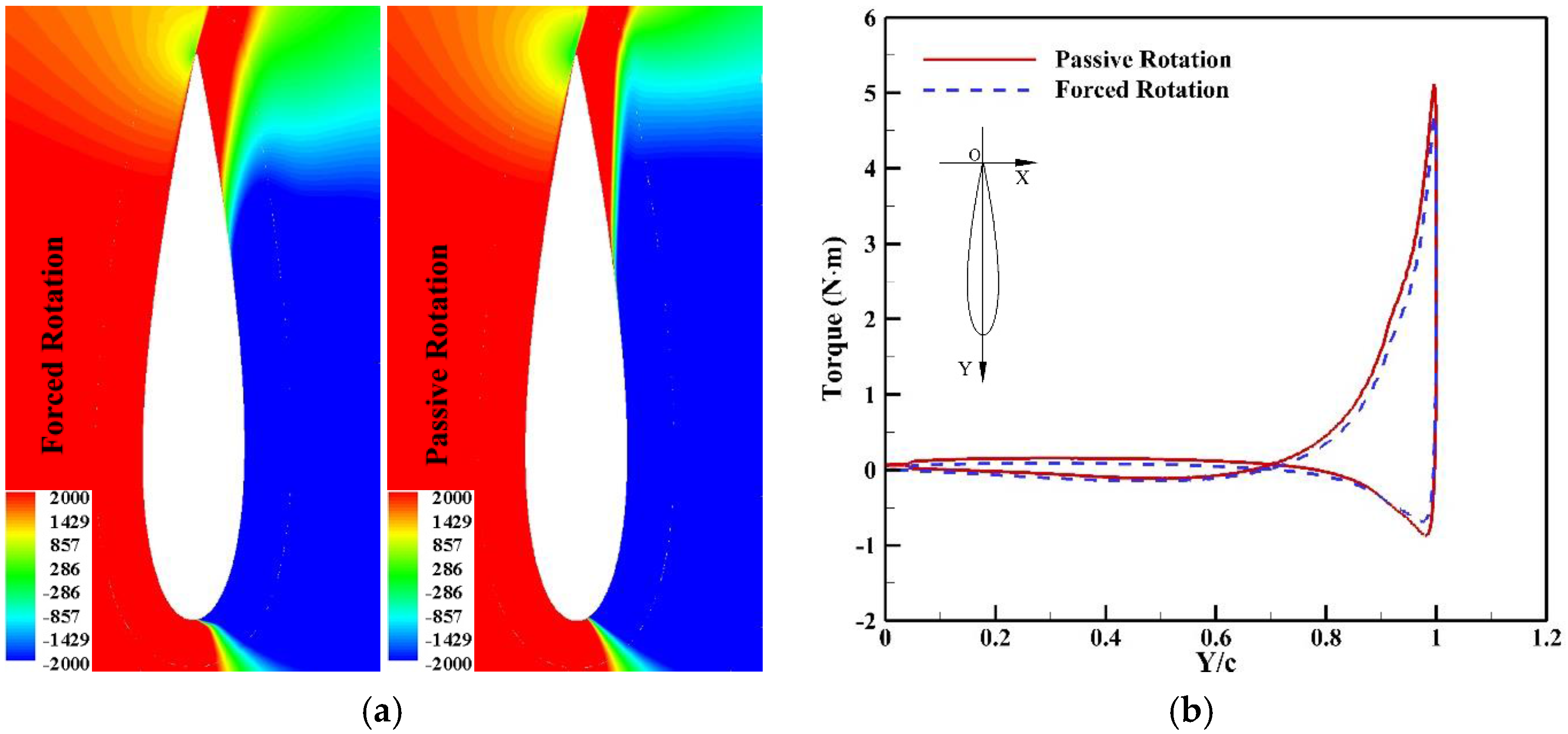
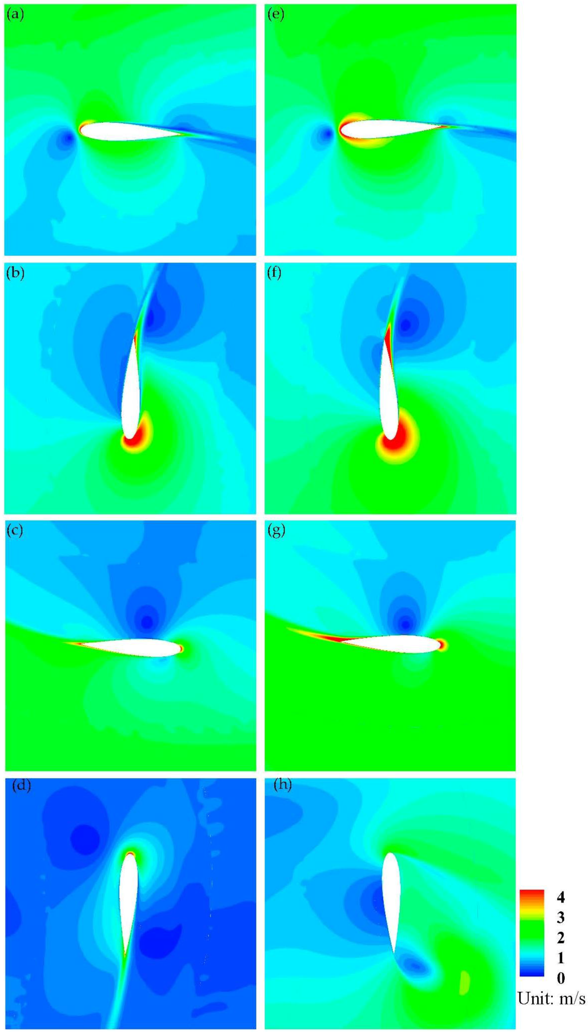
4.1. Calculations without the System Loads

In the calculations without the system loads, T_S is set as zero. The VAT rotor is driven by the hydrodynamic torque generated by the incident flow. To demonstrate the difference in the results of the numerical simulations of the traditional forced rotation (under a constant angular velocity) and the passive motion adopted in this study, a comparison of the velocity contours around a blade at various azimuth angles is performed, and is shown in Figure 3. The incident free velocity for both the modes is set as U_∞ = 1.5 m/s. The calculation of the passive rotation was carried out first. Because of the existence of the reserve torque, the hydrodynamic torque fluctuated near zero. Instead of continuous acceleration, an equilibrium state of the angular velocity was found. This averaged angular velocity (TSR = 4.72) was then used as the condition for performing the calculation in the case of forced rotation.

As shown in Figure 3a–c,e,f, the general characteristics of the flow structures around the blade at the azimuth angles of 0°, 90° and 180° for the two rotation modes are similar. The high speed area at both leading and trailing edges of the blade in the case of passive rotation is larger than that in the case of the forced rotation. Moreover, the low speed area near the sides of the blade, in the case of passive rotation, is smaller than that in the case of forced rotation.

As shown in Figure 3d, at the azimuth angle of 270°, the blade is forced to rotate in a relatively low speed area, which is in the wake area of the rotor. The flow velocities around the blade are higher than those in the other areas. Especially at the leading and trailing edges of the blade, the forcing effect is evident. On the other hand, as shown in Figure 3h, the flow velocities outside the rotor are relatively high for the passive rotation. A vortex can also be observed at the trailing edge in the case of passive rotation. Therefore, the difference in the flow structure between the passive and forced rotations is observed mainly in the wake area of the rotor. Compared to the flow dragged by the forced blade, the flow pushes and drags the blade more significantly in the passive mode when the blade rotates to the wake of the rotor.

A time history of the instantaneous torques under no-load condition in the starting process is shown in Figure 4. The incident free velocity is U_∞ = 1.5 m/s and the moment of inertial is I = 10 kg·m². It can be seen that the torques of the individual blades are disordered before t = 4.0 s during acceleration. After that moment, the equilibrium state is predicted for both the individual and total torques. The positive peak of the total torque is reduced to 42% of that of an individual blade because of the reverse torques from the other two blades.

The effect of the incident flow velocity on the rotation speed of the rotor is shown in Figure 5. Even without any external resistance, the rotor fails to self-start at the flow velocity U_∞ = 0.5 m/s, and keeps switching between “the start and stop” states. As shown in Figure 5a, the equilibrium state is predicted earlier when the incident velocity is higher. The equilibrium RPM (revolution per minute), which varies from 90 to 217, also increases as the incident velocity increases. As shown in Figure 5b, except the velocity condition of 0.5 m/s, the equilibrium TSRs at different incident velocities tend to be close (varying from 4.53 to 4.72). The fluctuation ratios of the rotation speeds in these cases are all less than 1%. This indicates that the incident flow velocity has only a small effect on the TSR of the Darrieus turbine’s rotor under no-load condition if the turbine can self-start.

The hydrodynamic performance analysis is shown in Figure 6; only three incident–velocity values are shown in the figure to illustrate the comparison clearly. As shown in Figure 6a, the total torque can increase up to 610 N·m and 263 N·m at the incident velocities of 2.5 m/s and 1.5 m/s, respectively, in the acceleration stage. In the equilibrium stage, the positive peak-values of the total torque at the above two velocities are 111 N·m and 43 N·m, respectively. The time averaged values of the total torque converge to zero. Moreover, the total torque at U_∞ = 0.5 m/s keeps fluctuating near zero throughout the time domain. It can be seen in Figure 6b that the peak value of positive C_p for U_{∞ =} 1.5 m/s in the equilibrium stages is 0.36, which is slightly larger than that for U_∞ = 2.5 m/s (C_p = 0.31). These results indicate that the passive model used in this study can accurately simulate the rotor motion under no-load conditions.

The effect of moment of inertia on the hydrodynamic performance of the VAT rotor is shown in Figure 7. The incident free velocity is set as 1.5 m/s. As expected, the rotor with a lower moment of inertia finishes the self-starting process earlier (Figure 7a). The averaged peak values of the torques in the equilibrium stage for the three values of moment of inertia are very close. The averaged-value of the peak torque for I = 1.0 kg·m² is slightly lower than those for the other two values of moment of inertia. As shown in Figure 7b, the time-averaged TSRs in the equilibrium stage for different moment of inertia are also close. The fluctuation in the TSR for I = 1.0 kg·m² is much larger than that for the other cases, because the rotor with a lower moment of inertia is more sensitive to variations in the torque. The results also indicate that the rotors with different moment of inertia values will achieve a similar rotation speed under no-load conditions.

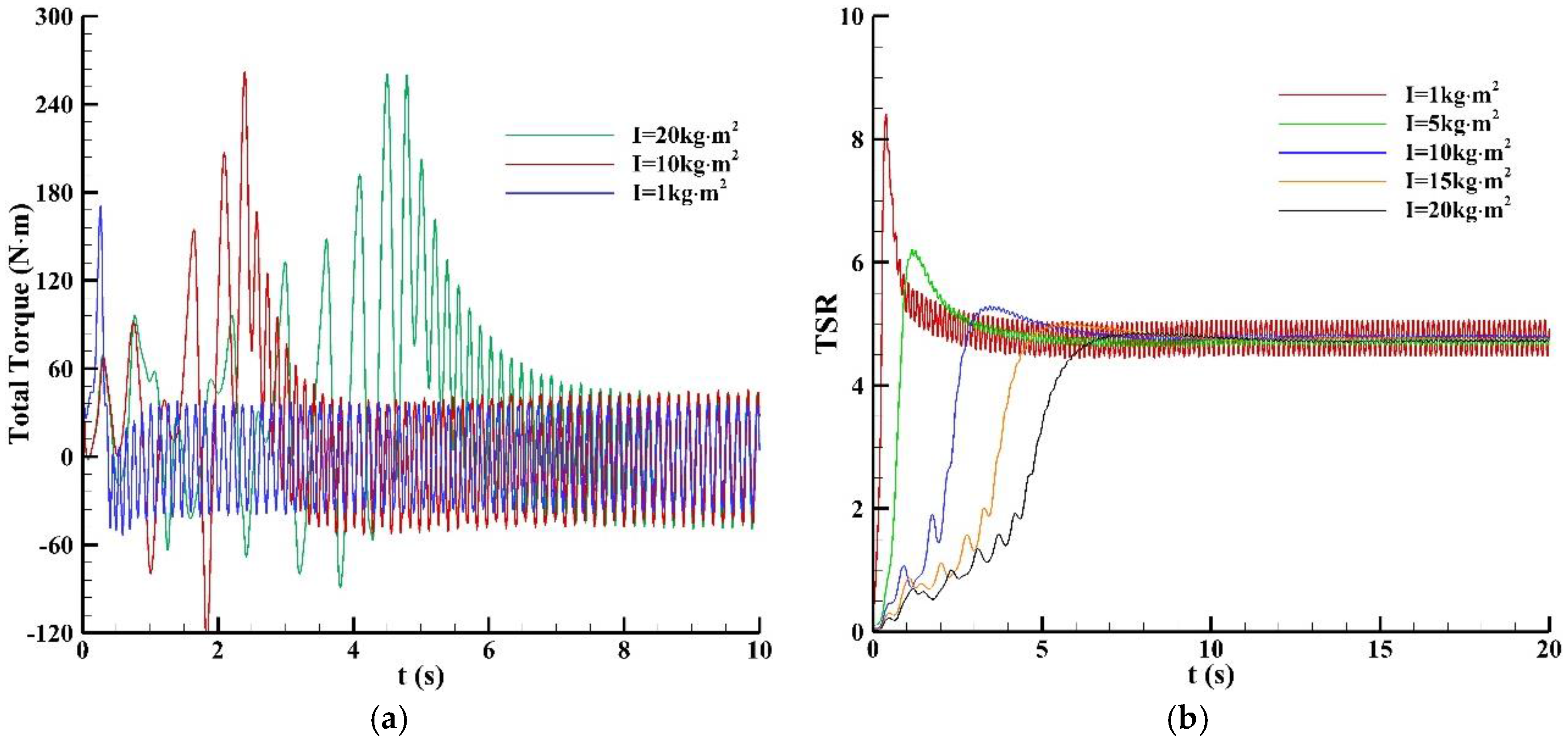
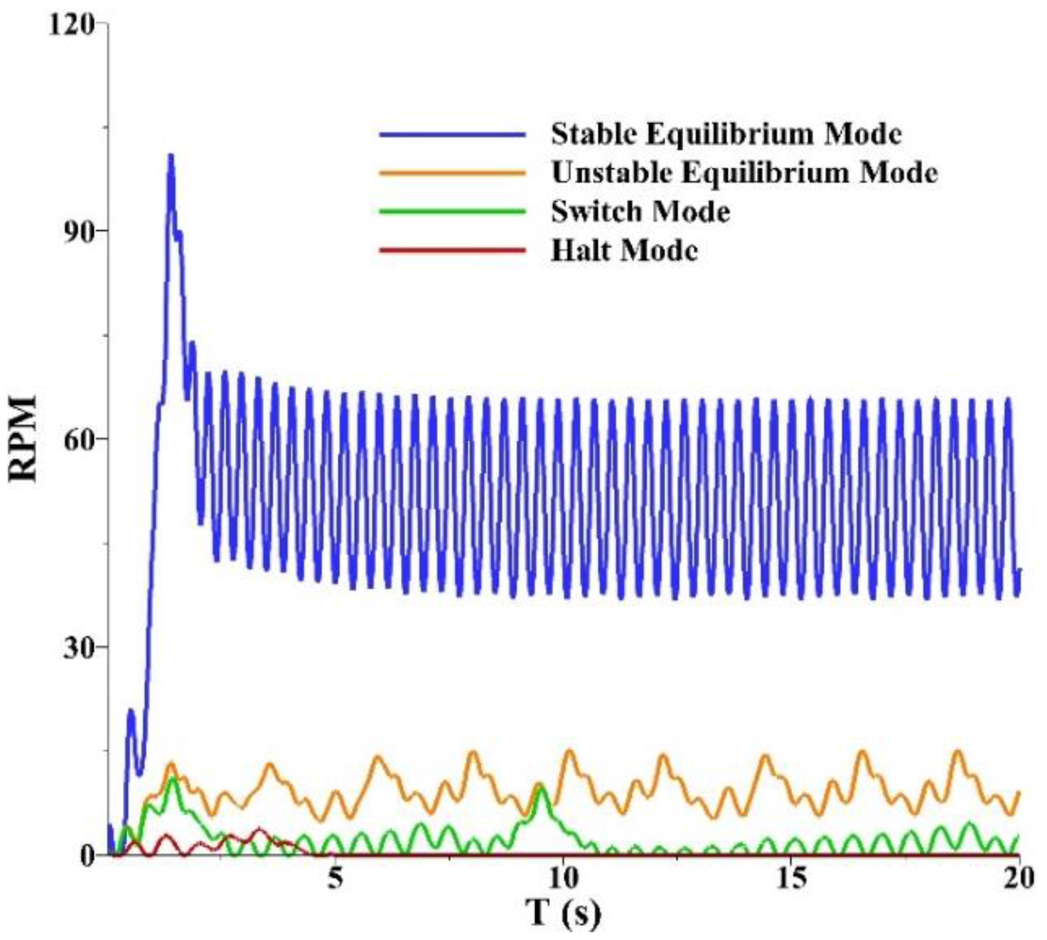
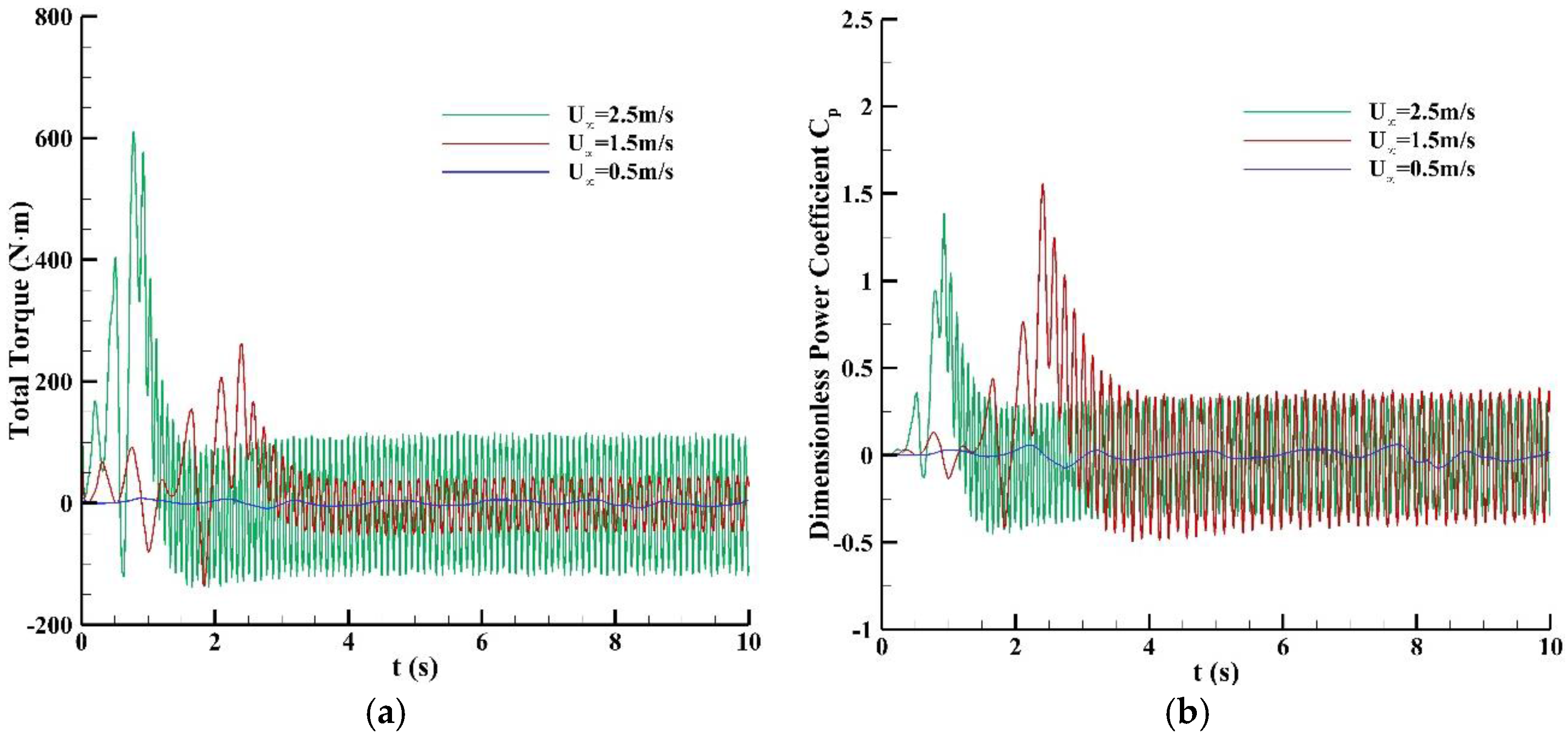
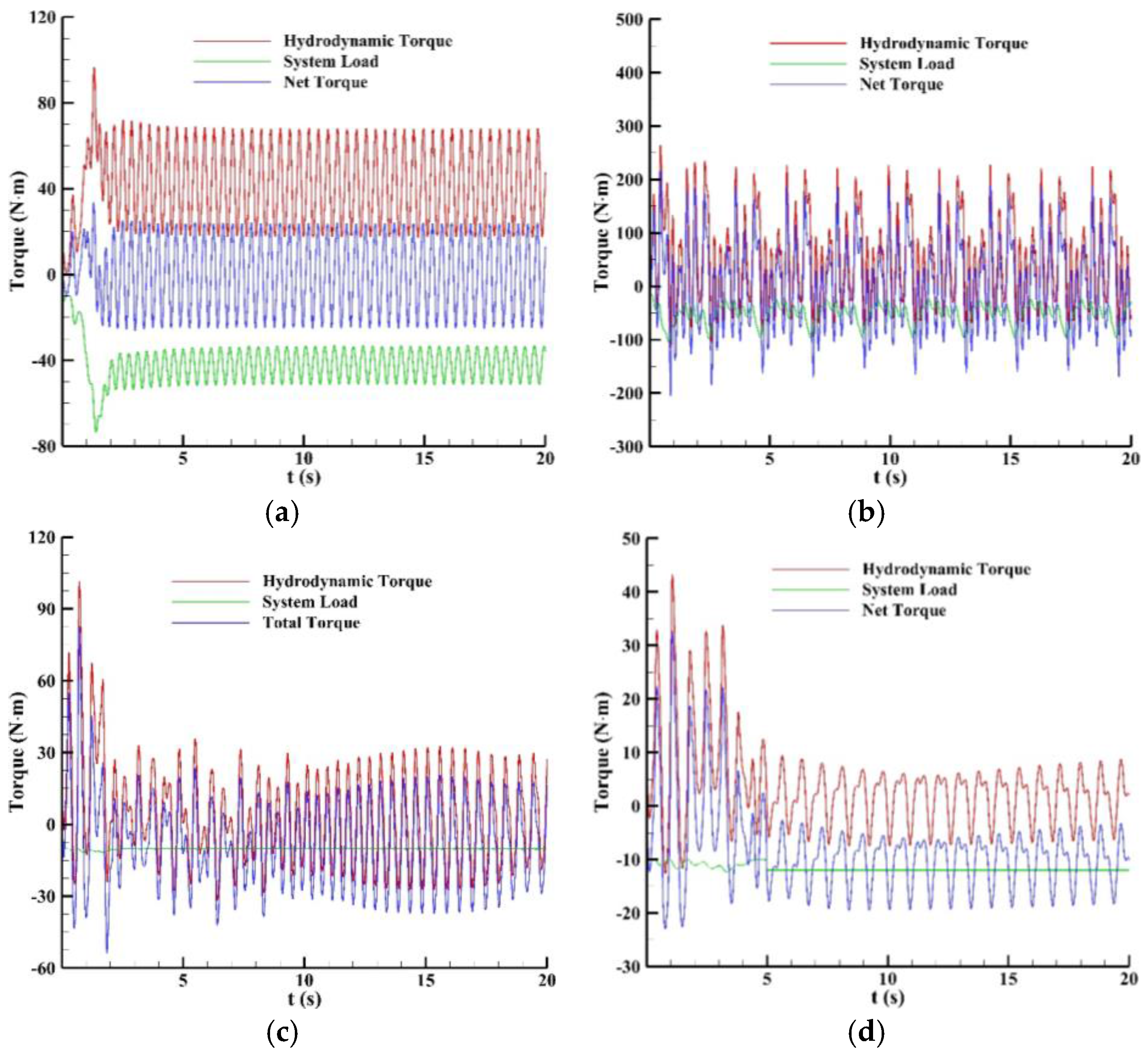
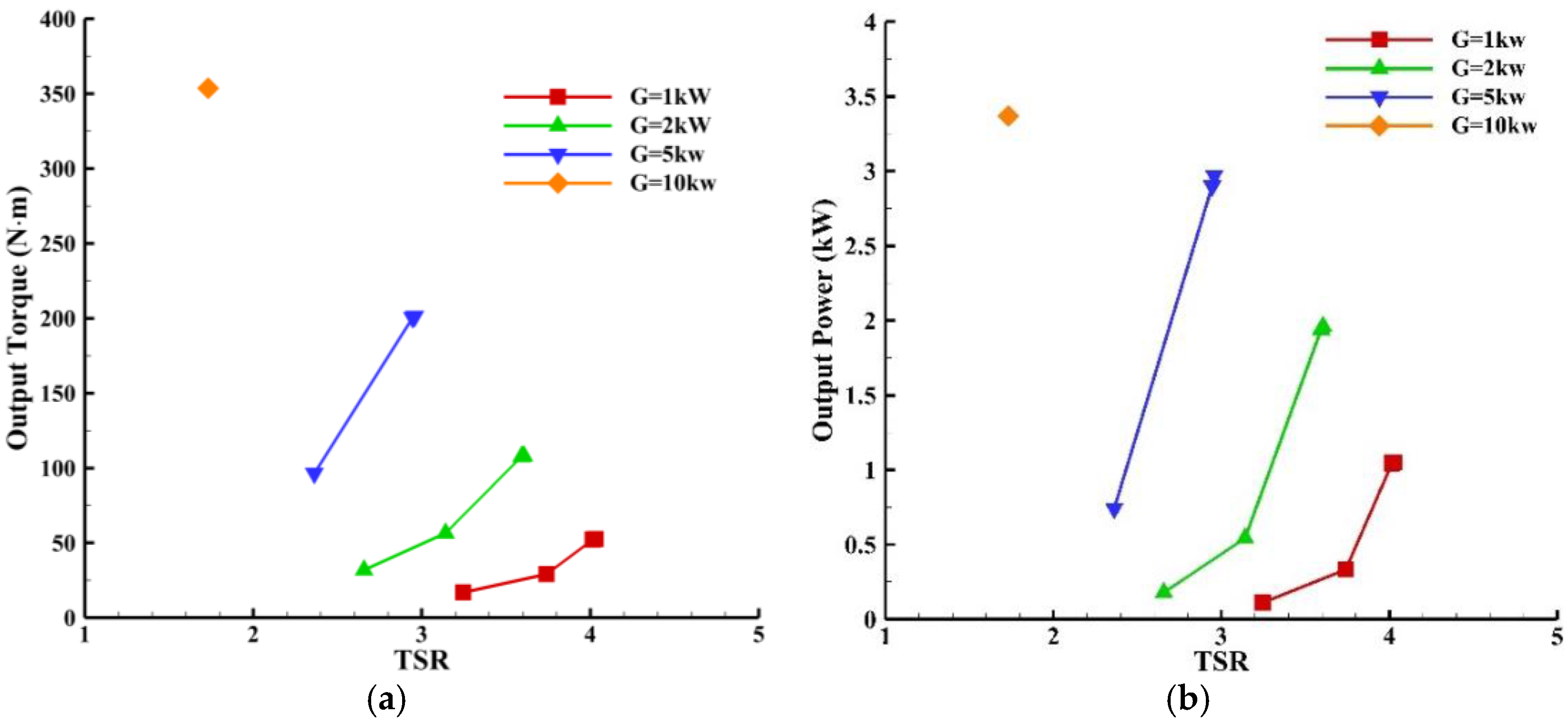
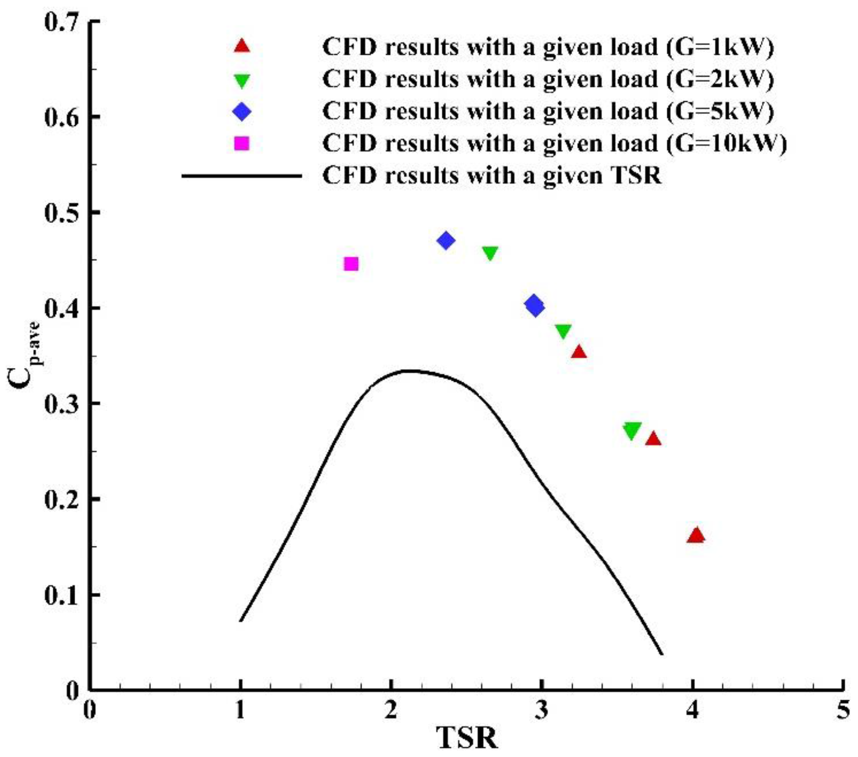
4.2. Calculations with the System Loads

In the calculation cases with the system loads, not all the entire drive train was considered and only the electric generator with necessary connectors (the bearing and clutch) were used to provide the resistance loads. A typical series of PMSG, widely employed for wind energy and tidal stream energy utilization in China [32], were used to provide the input system loads, which have a linear relationship with the rotation speed. Considering the output torque of the rotor in the forced and passive rotation cases, four installed capacities G were chosen: 1 kW, 2 kW, 5 kW and 10 kW. The values of initial torque and constant ratio k for each G are listed in

Table 2. Calculating parameters for different generators.

Installed Capacity G (kW)	Rated Rotation Speed (RPM)	Initial Torque (N·m)	Constant Ratio k (N·m·s/rad)
1	200	1.5	2.6
2	200	2.0	6.0
5	250	4.5	13.6
10	150	13.0	40.8

. The friction loads of the generator are mainly determined by the internal configurations and connections [33]. The generators with different installed capacities (from 1 kW to 10 kW) considered in this study have the same outline shape and internal configurations and connections [32], and the bearings and connecting components are all assumed to be same. Thus, the friction loads from the driven train are set as 10 N·m for all the generators. Three values of moment of inertia (1 kg·m², 10 kg·m² and 20 kg·m²) and three incident free velocities (1.0 m/s, 1.5 m/s and 2.5 m/s) were employed. Hence, there was a total of 36 cases in the calculations with system loads.

Four self-starting modes were found in the calculations with system loads: (a) Stable Equilibrium Mode (SEM); (b) Unstable Equilibrium Mode (UEM); (c) Switch Mode (SM); (d) Halt Mode (HM). The typical curves for these four modes are plotted in Figure 8. For the SEM (Condition: U_∞ = 1.0 m/s, I = 1 kg·m², G = 2 kW), after a quick increase during the initial stage, the rotation speed follows a sinusoidal shape curve and reaches a stable equilibrium state; For the UEM (Condition: U_∞ = 1.5 m/s, I = 20 kg·m², G = 1 kW), the rotation speed of the rotor is far less than that for the SEM. Furthermore, the rotor speed still shows periodic variation characteristics after 12 s; For the SM (Condition: U_∞ = 1.5 m/s, I = 20 kg·m², G = 5 kW), the rotation speed variation shows that the rotor keeps switching between the start and stop states and fails to self-start; For the HM (Condition: U_∞ = 1.0 m/s, I = 20 kg·m², G = 2 kW), the rotor tries to rotate at the initial stage, then quickly halts, and finally fails to restart again.

The time histories of the torques corresponding to the four modes during the self-starting process are shown in Figure 9. Figure 9a shows that after the acceleration during the initial stage, the hydrodynamic torque and the system load show a sinusoidal shape in the equilibrium state. The total torque also fluctuates near zero to enable the rotor to rotate stably. In Figure 9b, periodic variations of the hydrodynamic torque, system load, and total torque can be observed, which cause the rotor to rotate in an unstable equilibrium state. For the SM in Figure 9c, the hydrodynamic torque is very low. Although a relatively stable total-torque can be generated, the rotation speed is low, and this causes the rotor to switch between the start and stop states. Since there is no increase in the net torque, the rotor cannot be made to accelerate anymore. As shown in Figure 9d, the hydrodynamic torque decreases quickly and causes the net torque to decrease to a negative value. After the rotor halts, the system load will be the sum of the friction and initial torques, and the hydrodynamic torque during the resting state fails to generate positive net torque and restarts the rotor rotation again.

The operating performance of the VAT rotor is given in Figure 10. Only the SEM results are shown to demonstrate the rotor performance under the stable equilibrium state after self-starting. The time-averaged values of output torque at the stable equilibrium stage are shown in Figure 10a and are used to calculate the output power in Figure 10b. It can be seen that the rotor linked to a generator with a smaller installed capacity has a higher speed and delivers lower torque and power. For a given generator, a larger TSR will enable the rotor to generate more power. The highest output-power predicted in this study is 3.37 kW under the condition: U_∞ = 2.5 m/s, I = 1 kg·m², and G = 10 kW.

A typical comparison of the pressure and hysteresis loop of vertical torques around a blade in the forced and passive rotation cases is shown in Figure 11. The calculation conditions are as follows: U_∞ = 1.5 m/s, I = 1 kg·m², and G = 5 kW. The averaged TSR for passive rotation is 2.36, which is used as the fixed TSR for forced rotation. The instantaneous azimuth angle of the blade is 90°. The contours of pressure distribution around the blade airfoil are illustrated in Figure 11a. It can be seen that the general distribution of the pressure around the airfoil is similar. The main difference can be found in the domain of negative pressure at the left side of the blade.

The hysteresis loop of vertical torques generated on the blade at the azimuth angle of 90° for two rotation conditions are compared in Figure 11b. The downward direction is defined as the positive direction of the vertical torques. The direction of the hysteresis loop is anticlockwise. The torque distribution characteristics for the forced and passive rotation conditions are similar. A peak can be found at the leading edge in the negative pressure domain. Except a small section of the leading edge in the positive pressure domain, most torques generated on the blade cells in the vertical direction in the passive rotation case are slightly higher than those for the forced rotation condition. In this case, the resultant torque in the vertical direction for passive rotation is 43 N·m higher than that for the forced rotation condition.

A comparison of the predicted values of C_p-ave for the passive and forced rotation conditions is shown in Figure 12. As in the case of Figure 10, only the results of the simulations for passive rotation for the SEM are shown. It can be seen that the curve of C_p-ave in the passive rotation condition has a varying trend similar to that in the case of the forced rotation. A peak value of C_p-ave is predicted as 0.47 under the condition of U_∞ = 1.5 m/s, I = 1 kg·m², and G = 5 kW. The TSR in the equilibrium state is 2.36. Overall, the C_p-ave in the passive simulation is, on average, 38% higher than those calculated in the forced rotation cases, as can be seen in Figure 11, which is caused by a higher torque generated by the blade. The results indicate that the previous studies that used the methodology of a given rotation speed have underestimated the real operating performance of the VAT rotor without any controls.

On the other hand, it should be pointed out that the 2D numerical model has an inevitable disadvantage in ignoring some realistic frictions, parasitic drags and other 3D effects. Therefore, not the absolute values but the relative values of the power coefficient in Figure 12 may provide more reference value to the comparison of the numerical simulations for the passive and forced rotation conditions in this study. Moreover, a usable electricity output needs a relative stable rotation speed of the rotor and the generator. It means that the big variation shown in Figure 9 should be controlled artificially to match the need of the electricity generation and output.

The self-starting modes for all the calculation cases are listed in

Table 3. Summary of self-starting modes.

Free Velocity (m/s)	Moment of Inertia (kg·m2)	Installed Capacity (kW)	Mode of Self-Starting
1	1	1	SEM
		2	SEM
		5	HM
		10	HM
1.5	1	1	SEM
		2	SEM
		5	SEM
		10	SM
2.5	1	1	SEM
		2	SEM
		5	SEM
		10	SEM
1	10	1	HM
		2	HM
		5	HM
		10	HM
1.5	10	1	SM
		2	SM
		5	SM
		10	SM
2.5	10	1	SEM
		2	SEM
		5	SEM
		10	SM
1	20	1	HM
		2	HM
		5	HM
		10	HM
1.5	20	1	UEM
		2	UEM
		5	SM
		10	SM
2.5	20	1	SEM
		2	SEM
		5	UEM
		10	UEM

. When the moment of inertia is low, the rotor can drive the generator with smaller values of G. For a large value of G, the mode changes from HM to SM or SEM as the incident velocity increases; For a medium moment of inertia (I = 10 kg·m²), the rotor cannot drive any generator at U_∞ = 1.0 m/s. In addition, the self-starting mode is the SM at U_∞ = 1.5 m/s. The rotor can drive the generators at U_∞ = 2.5 m/s except the one with G = 10 kW; For a large moment of inertia (I = 20 kg·m²), the rotor fails to drive any generators when the velocity is low (U_∞ = 1.0 m/s) and can drive the generator with a small installed capacity (G = 1 kW, or 2 kW) when the velocity is higher.

5. Conclusions

In this study, a 2D numerical model based on the CFD software ANSYS-Fluent was established to investigate the self-starting performance of the Darrieus straight-bladed VAT rotor. The passive rotation driven directly by the incident flow could be simulated numerically. The system loads, including the friction torque, initial torque and reverse torque during the rotation of the generator were also considered in the numerical model. The model was validated by the experimental data of the self-starting process of the Darrieus wind turbine.

A comparison of the flow structures indicates that the blades were pushed by the flow more significantly in the wake area of the rotor in the simulations of the passive rotation condition. Under no-load condition, the free velocity and the moment of inertia of the rotor were found to have little effect on the TSR. Under system load conditions, there were four modes of self-starting: SEM, UEM, SM and HM. The highest power predicted in this study is 3.37 kW. A larger negative pressure domain was observed around a blade at the azimuth angle of 90° for the passive rotation case. This will cause the generation of a higher working torque at the leading edge, especially in the negative pressure domain for passive rotation. Consequently, the averaged dimensionless power coefficient in the passive simulation was, on average, 38% higher than those derived from the simulation of forced rotation with the same TSR. A rotor with a lower inertia can be expected to deliver more torque and power for tidal stream conversion.

It should be pointed out that the 2D numerical model has ignored some important 3D effects, including the parasitic drags and frictions. We believe that this yielded an overestimation on the prediction of the power coefficient. In the future work, this numerical methodology on the flow-driven self-starting of VAT should be applied in the 3D model to recruit for a more precise prediction on the passive rotation of the Darrieus turbine. The experimental study on the self-starting of VAT needs to be conducted in the water flow tank to provide more reliable data.

References

1. Jesch, L.F.; Walton, D. Reynolds number effects on the aerodynamic performance of a vertical axis wind turbine. In Proceedings of the 3rd International Symposium on Wind Energy Systems, Lyngby, Denmark, 26–29 August 1980.
2. Kentfield, J.A.C. A cycloturbine with automatic, self-regulating, blade pitch control. In Proceedings of the 4th ASME Wind Turbine System, Dallas, TX, USA, 17–21 February 1985.
3. Kentfield, J.A.C. Theoretically and experimentally obtained performances of gurney-flap equipped wind turbines. Wind Eng. 1996, 18, 63–71. [Google Scholar]
4. Dominy, R.; Lunt, P.; Bickerdyke, A.; Dominy, J. Self-starting capability of a Darrieus turbine. Proc. Inst. Mech. Eng. A J. Power Energy 2007, 221, 111–120. [Google Scholar] [CrossRef] [Green Version]
5. Baker, J.R. Features to aid or enable self starting of fixed pitch low solidity vertical axis wind turbines. J. Wind Eng. Ind. Aerodyn. 1983, 15, 369–380. [Google Scholar] [CrossRef]
6. Kirke, B.K. Evaluation of Self-Starting Vertical Axis Wind Turbines for Stand-Alone Applications. Ph.D. Thesis, School of Engineering, Griffith University, Nathan, QLD, Australia, 1998. [Google Scholar]
7. Hill, N.; Dominy, R.; Ingram, G.; Dominy, J. Darrieus turbines: The physics of self-starting. Proc. Inst. Mech. Eng. A J. Power Energy 2009, 223, 21–29. [Google Scholar] [CrossRef]
8. Biadgo, A.M.; Simonovic, A.; Komarov, D.; Stupar, S. Numerical and analytical investigation of vertical axis wind turbine. FEM Trans. 2013, 41, 49–58. [Google Scholar]
9. Nguyen, C.C.; Le, T.H.H.; Tran, P.T. A numerical study of thickness effect of the symmetric NACA 4-digit airfoils on self starting capability of a 1 kW H-type vertical axis wind turbine. Int. J. Mech. Eng. Appl. 2015, 3, 7–16. [Google Scholar]
10. Beri, H.; Yao, Y.X. Effect of camber airfoil on self starting of vertical axis wind turbine. J. Environ. Sci. Technol. 2011, 4, 302–312. [Google Scholar] [CrossRef]
11. Batista, N.C.; Melicio, R.; Matias, J.C.O.; Catalao, J.P.S. Self-start evaluation in lift-type vertical axis wind turbines: Methodology and computational tool applied to asymmetrical airfoils. In Proceedings of the 2011 International Conference on Power Engineering, Energy and Electrical Drives, Torremolinos, Spain, 11–13 May 2011.
12. Seralathan, S.; Micha, P.T.; Thangavel, S.; Pradeep, G.P. Numerical studies on the effect of cambered airfoil blades on self starting of vertical axis wind turbine Part 2: NACA 0018 and NACA 63415. Appl. Mech. Mater. 2015, 787, 245–249. [Google Scholar] [CrossRef]
13. Singh, M.A.; Biswas, A.; Misra, R.D. Investigation of self-starting and high rotor solidity on the performance of a three S1210 blade H-type Darrieus rotor. Renew. Energy 2015, 76, 381–387. [Google Scholar] [CrossRef]
14. Dumitrache, A.; Frunzulica, F.; Dumitrescu, H.; Suatean, B. Influences of some parameters on the performance of a small vertical axis wind turbine. Renew. Energy Environ. Sustain. 2016, 1, 1–5. [Google Scholar] [CrossRef]
15. Sengupta, A.R.; Biswas, A.; Gupta, R. Studies of some high solidity symmetrical and unsymmetrical blade H-Darrieus rotors with respect to starting characteristics, dynamic performances and flow physics in low wind streams. Renew. Energy 2016, 93, 536–547. [Google Scholar] [CrossRef]
16. Batista, N.C.; Melicio, R.; Mendes, V.M. F.; Calderon, M.; Ramiro, A. On a self-start Darrieus wind turbine: Blade design and field tests. Renew. Sustain. Energy Rev. 2015, 52, 508–522. [Google Scholar] [CrossRef]
17. Zhang, L.X.; Pei, Y.; Liang, Y.B.; Zhang, F.Y.; Wang, Y.; Meng, J.J.; Wang, H.R. Design and implementation of straight-bladed vertical axis wind turbine with collective pitch control. In Proceedings of the 2015 IEEE International Conference on Mechatronics and Automation, Beijing, China, 2–5 August 2015.
18. Liang, Y.B.; Zhang, L.X.; Li, E.X.; Zhang, F.Y. Blade pitch control of straight-bladed vertical axis wind turbine. J. Cent. South Univ. 2016, 23, 1106–1114. [Google Scholar] [CrossRef]
19. P’Yankov, K.S.; Toporkov, M.N. Mathematical modeling of flows in wind turbines with a vertical axis. Fluid Dyn. 2014, 49, 249–258. [Google Scholar] [CrossRef]
20. Naoi, K.; Tsuji, K.; Shiono, M.; Suzuki, K. Study of characteristics of Darrieus-type straight-bladed vertical axis wind turbine by use of ailerons. J. Ocean Wind Energy 2015, 2, 107–112. [Google Scholar] [CrossRef]
21. Bos, R. Self-Starting of a Small Urban Darrieus Rotor—Strategies to Boost Performance in Low-Reynolds-Number Flows. Master’s Thesis, Faculty of Aerospace Engineering, Delft University of Technology, Delft, The Netherlands, 2012. [Google Scholar]
22. Untaroiu, A.; Wood, H.G.; Allaire, P.E.; Ribando, R.J. Investigation of self-starting capability of vertical axis wind turbines using a computational fluid dynamics approach. J. Sol. Energy Eng. 2011, 133, 041010. [Google Scholar] [CrossRef]
23. Rossetti, A.; Pavesi, G. Comparison of different numerical approaches to the study of the H-Darrieus turbines start-up. Renew. Energy 2013, 50, 7–19. [Google Scholar] [CrossRef]
24. Zhu, J.Y.; Huang, H.L.; Shen, H. Self-starting aerodynamics analysis of vertical axis wind turbine. Adv. Mech. Eng. 2015, 7, 1–12. [Google Scholar] [CrossRef]
25. Dumitrescu, H.; Cardos, V.; Malael, I. The physics of starting process for vertical axis wind turbines. In CFD for Wind and Tidal Offshore Turbines, 1st ed.; Eerrer, E., Montlaur, A., Eds.; Springer: Cham, Switzerland, 2015; pp. 69–81. [Google Scholar]
26. Le, T.Q.; Lee, K.S.; Park, J.S.; Ko, J.H. Flow-driven rotor simulation of vertical axis tidal turbines: A comparison of helical and straight blades. Int. J. Nav. Archit. Ocean Eng. 2014, 6, 257–268. [Google Scholar] [CrossRef]
27. Zhang, X.W.; Zhang, L.; Wang, F.; Zhao, D.Y.; Pang, C.Y. Research on the unsteady hydrodynamic characteristics of vertical axis tidal turbine. China Ocean Eng. 2014, 28, 95–103. [Google Scholar] [CrossRef]
28. Lunt, P.A. An Aerodynamic Model for a Vertical-Axis Wind Turbine. Master’s Thesis, School of Engineering, University of Durham, Durham, UK, 2005. [Google Scholar]
29. Worasinchai, S.; Ingram, G.L.; Dominy, R.G. The physics of H-Darrieus turbine starting behavior. J. Eng. Gas Turbines Power 2016, 138, 062605. [Google Scholar] [CrossRef]
30. Marsh, P.; Ranmuthugala, D.; Penesis, I.; Thomas, G. Three-dimensional numerical simulations of straight-bladed vertical axis tidal turbines investigating power output, torque ripple and mounting forces. Renew. Energy 2015, 83, 67–77. [Google Scholar] [CrossRef]
31. Liu, Z.; Qu, H.L.; Shi, H.D.; Hu, G.X.; Hyun, B.S. Application of 2D numerical model to unsteady performance evaluation of vertical-axis tidal current turbine. J. Ocean Univ. China 2016, 15, 1–10. [Google Scholar] [CrossRef]
32. PMSG Product List. Available online: http://www.tianlongpmg.com/enindex.php (accessed on 8 July 2016).
33. Alcorn, R.; O’Sullivan, D. Electrical Design for Ocean Wave and Tidal Energy Systems. In IET Renewable Energy Series 7; The Institute of Engineering and Technology: London, UK, 2014. [Google Scholar]
Figure 1. 2D computational domain, boundaries and meshes.
Energies 09 00789 g001
Figure 2. Comparison of variations in angular velocities for the Darrieus wind turbine.
Energies 09 00789 g002
Figure 3. Comparison of velocity contours around a blade. Forced rotation: (a) 0°(360°); (b) 90°; (c) 180°; (d) 270°; Passive rotation: (e) 0°(360°); (f) 90°; (g) 180°; (h) 270°.
Energies 09 00789 g003
Figure 4. Time history of the instantaneous torques during the starting process.
Energies 09 00789 g004
Figure 5. Effects of the incident flow velocity on the rotation speed (No-load condition): (a) Revolution per minute (RPM); (b) Tip-speed-ratio (TSR).
Energies 09 00789 g005
Figure 6. Effects of the incident free velocity on the hydrodynamic performance (No-load condition): (a) Torque; (b) Cp.
Energies 09 00789 g006
Figure 7. Effects of the moment of inertia on the hydrodynamic performance (No-load condition): (a) Torque; (b) TSR.
Energies 09 00789 g007
Figure 8. Four typical modes of self-starting processes under the load conditions.
Energies 09 00789 g008
Figure 9. Time histories of torques during self-starting under the load conditions: (a) Stable Equilibrium Mode (SEM); (b) Unstable Equilibrium Mode (UEM); (c) Switch Mode (SM); (d) Halt Mode (HM).
Energies 09 00789 g009
Figure 10. Operating performance of the VAT rotor: (a) Output Torque; (b) Output Power.
Energies 09 00789 g010
Figure 11. Comparison of hydrodynamics between the forced and passive rotations: (a) Pressure Contour; (b) Hysteresis loop of torques.
Energies 09 00789 g011
Figure 12. Comparison of Cp-ave under passive and forced rotation conditions.
Energies 09 00789 g012