
Accuracy Enhancement of Mixed Power Flow Analysis Using a Modified DC Model

Department of Electrical Engineering, Kyungpook National University, Daegu 41566, Korea
Energies 2016, 9(10), 776; https://doi.org/10.3390/en9100776
Submission received: 1 August 2016
/
Revised: 9 September 2016
/
Accepted: 22 September 2016
/
Published: 26 September 2016
(This article belongs to the Special Issue Electric Power Systems Research 2017)
Abstract
:The mixed power flow analysis method decreases the computational complexity and achieves a high level of simulation accuracy. The mixed approach combines the ac with the dc power flow models, depending on the area of interest. The accurate ac model is used in the study area of interest to obtain high simulation accuracy, while the approximate dc model is used in the remainder of the system to reduce the required computations. In the original mixed approach, the errors originating from the use of the dc model may propagate to the area of interest where accurate simulation outcomes are required; thus, the simulation accuracy might not be satisfactory. This paper presents a new method of enhancing the simulation accuracy of the mixed power flow analysis using available information. In the proposed approach, a modified dc model is used instead of the traditional one and is constructed from an initial base-case ac solution. The new dc model compensates for the errors originating from the neglect of the real power losses and the assumption of a flat voltage magnitude in the conventional dc model. Thus, the proposed method can improve the simulation accuracy in the area of interest. The superior computational benefits can also be preserved by maintaining linear characteristics of the dc model. Case studies with the IEEE 118-bus system are provided to validate the enhanced accuracy of the proposed method.
1. Introduction
Steady-state power flow analysis is a fundamental tool and the most frequently used routine in power system planning, operations, and control. It provides the bus voltages of each bus, and the power flows through a transmission network for a specified load and generator information. With this analysis, various contingencies and expansion plans can be carefully explored, and security indexes such as component overloading and power transfer capability can be evaluated. However, owing to interconnections, modern electric power systems have become increasingly complex, large-scale systems comprising numerous components. Power system equations are inherently nonlinear. The complexity issues in the analysis have grown and become even more burdensome with the recent integration of renewable energy sources. Thus, the need for the development of rapid and precise power system analysis tools has become critical [1].
The primary and the most accurate approach for power flow analysis models the electric power networks with a set of nonlinear power balance equations; this is typically referred to as the ac model. Based on Kirchhoff’s law and the definition of complex power, nonlinear real and reactive power balance equations are derived for each bus. A large number of equations are required to represent the modern large power systems. The set of nonlinear equations is usually solved using iterative techniques such as Newton’s method. Hence, the ac model is computationally expensive, especially for the contingency analysis of large power systems [2].
Complexity reduction in power flow studies has been attempted with many approximate models, which are based on the physical properties of the power systems [3,4,5,6]. The most common examples include the decoupled and dc power flows. The decoupled power flow utilizes a remarkable property of the power system: the interactions between the real power and the bus voltage angle and the interactions between the reactive power and the bus voltage magnitude are very strong. This property simplifies the Jacobian matrix, which results in rapid power flow solutions. While the decoupled method requires more iterations to converge, it usually provides much faster results than the conventional Newton’s method with the ac model [6].
Furthermore, the dc model is the simplest and fastest power flow modeling approach. The dc model focuses only on the real power flow, and it changes the nonlinear power flow equations to linear ones. Therefore, the number of equations can be reduced and iterative techniques are not required to find the power flow solutions [7]. Because of its superior computational benefits, this traditional dc model is widely used in various power system applications. Examples include security constrained unit commitment (SCUC), economic dispatch, and real-time contingency analysis. However, the dc model offers approximate solutions only, particularly when the X/R ratios are not big enough or the voltage profiles are not uniform [8].
Many different versions of the dc power flow models have been proposed [8,9,10,11,12]. These can be classified into hot-start and cold-start models. The hot-start model is formulated when the initial ac power flow solution is available, while the cold-start models are derived when the initial ac solution is not available. Hot-start models show better simulation accuracies because the inaccuracy of the dc model can be compensated using the initial ac solution. The hot-start models are often used in short- and medium-term operations and planning simulations. On the contrary, cold-start models are state-independent because the base-case information is not incorporated. Thus, flat voltages are approximated and net losses are neglected. The classical dc power flow is included in cold-start models. SCUC, financial right auction, and long term planning studies are typical applications of the cold-start models.
A hybrid power flow method has been proposed by the author [13]. The mixed approach uses a combination of ac and dc models, depending on the area of interest. The method aims to reduce the computational demands with the simpler dc model, as well as to maintain a high level of simulation accuracy using the accurate ac model. The mixed approach was originally developed based on the cold-start dc model. The errors originating from the use of the classical dc model may propagate to the area of interest where accurate simulation outcomes are required; thus, the simulation accuracy might not be satisfactory. Under certain power system conditions, a significant loss of simulation accuracy can occur if the original mixed approach is used. For power system operations and control where careful examination is required, inaccuracies may cause severe problems. For economic studies, even small errors in the power flow calculations may lead to substantial economic losses when aggregated over the year. A more robust approach to provide precise solutions should be developed.
In practical power system operations, various applications are investigated with prior knowledge about the present power system conditions including initially solved ac power flow solutions. The base-case ac solutions can be obtained from a state estimator, which is an EMS (Energy Management System) application program that identifies the current operating state of the system [14,15]. This additional information can be utilized to construct the hot-start dc models, which take the place of the cold-start model in the original mixed approach.
This paper presents a new method to enhance the simulation accuracy of the mixed power flow analysis. In the proposed method, the traditional dc model is modified by incorporating the base-case ac solution which is commonly available. The real power losses, which are neglected in the classical dc model, are compensated to maintain the overall system balance. In addition, the new approach includes the voltage magnitude information instead of the one-per-unit assumption. The modifications are helpful for minimizing the error propagation from the use of the traditional dc model. Thus, the simulation accuracy can be improved. The superior computational benefits can also be preserved with a linear formulation of the dc model.
The remainder of this paper is organized as follows. Section 2 presents a brief overview of the mixed power flow analysis. The enhanced method is proposed along with the problem definition in Section 3. Section 4 illustrates the simulation results using the IEEE 118-bus system. Various system conditions are studied to evaluate the performance of the proposed method. The conclusions are presented in Section 5.
2. Mixed Power Flow Analysis
In this section, the ac and dc models and the mixed approach are briefly explained.
2.1. AC Model
The ac power flow model shown in Equations (1) and (2) is the most accurate approach for modeling the steady-state behavior of balanced three-phase electric power networks. The real and reactive power balance equations are formulated for each bus. The complete set of nonlinear equations is solved with iterative numerical methods. Thus, the ac model introduces heavy computational burdens; however, it provides accurate solutions.
where , are the real and reactive power injection at bus k; is the voltage magnitude at bus k; is the voltage angle at bus k; is the real part of admittance matrix element ; is the imaginary part of admittance matrix element ; and superscript sp denotes the specified value.
2.2. DC Model
The dc model is the simplified version of the ac model, assuming a lossless network, one-per-unit voltage magnitudes, and small voltage angle variations, while completely ignoring the reactive power equations. With these assumptions, the real power equation in (1) can be modified to the simple linear equation in (3).
Since the equation is linear, the solution can be calculated directly; this means that the dc model always has a single solution. The linearity and the reduced number of equations allow the dc power flow model to compute the solutions much faster than the ac model. For locational marginal price (LMP) calculations in practical power systems, the dc power flow model was shown to be about 60 times faster than the ac model [7]. Because of the advantages in speed and robustness, the dc model has been an attractive tool for real-time market analyses and future expansion planning. However, the accuracy of the dc model solution is highly variable depending on the power system. An excellent simulation result can be obtained only if the underlying assumptions are satisfied. However, these assumptions cannot always be justified and sometimes might be unrealistic for practical power systems.
Many studies have been conducted to quantify the simulation accuracy of the dc model and to increase its performance [8,11,16]. It was observed in [8] that the main factors affecting the accuracy of the dc model are the flat voltage profile and the ignorance of real power losses. A satisfactory accuracy has been reported with hot-start models, which take the branch losses and bus voltages into account using the base-case ac power flow results or the historical data of the system [11,16]. These are state-dependent models. The hot-start model could maintain the same amount of MW losses in the entire system; thus, the total system power balance could be preserved without the need for generating additional power from a slack generator. A more advanced version even modifies the slope of the dc model linear equation corresponding to Bkm in Equation (3).
2.3. Mixed Approach
The mixed approach was proposed to take advantage of the best of both ac and dc models in terms of computational benefits and simulation accuracy. The approach first partitions the electric network into three subsystems, which are the internal system, the external system, and the boundary buses. The division is dependent on the areas of interest under study, and those are mutually exclusive. Then, it formulates the power flow problem by combining the ac model with the dc model. The detailed ac model in Equations (1) and (2) is used in the study area of interest and is called the internal system. The less-detailed dc model in Equation (3) is used in the external system, which is the remainder of the system. Thus, the approach aims to obtain accurate simulation outcomes in the internal system and to decrease computational demands by the use of the simplified dc model in the external system. The set of formulated equations can be solved using the well-known Newton–Raphson method. Figure 1 shows the overall procedure of the mixed approach.
The computational benefits of the mixed approach come from the reduced number of equations in the external system and the reduction of operations required for LU factorization and forward/backward substitution to solve the linear matrix equations. Simulation time is dependent on the ratio of the number of internal buses to external buses. With the IEEE 118-bus system in [17], the mixed approach, using a ratio in which the external system has about 1.5 times more buses than the internal system, can reduce the simulation time by half. More computational gain can be expected with larger power systems and larger dimensions of the external system compared to the internal one. Comprehensive details including speed, accuracy, and examples can be found in [13].
3. The Proposed Method
3.1. The Accuracy Problem
The mixed approach might have problems in the accuracy of the simulation outcomes, although an exact ac model is used in the internal system. Errors originating from the simplified dc model may be transferred to the internal system. In the original mixed approach, careful considerations were made to minimize the error propagation by formulating the ac power flow equations at the boundary buses composed of the boundaries between the two systems. However, the errors from the use of a dc model cannot be completely avoided under certain conditions, and the mixed approach fails to provide accurate simulation outcomes. The accuracy problem arises from the excessive approximations made in the dc model, especially from the neglect of the real power losses. Static power flow analysis assumes that the real and reactive powers are balanced in the entire system, and this means that the total generation is equal to the total consumption plus losses. Ignorance of the real power losses reduces the total amount of generation. Although the real power losses on a transmission line are relatively small, the cumulative sum of these losses might be significant, particularly when a large power system is under study. For example, if the external area does not have enough real power injections, the real powers required to maintain the system balance must be provided from the internal system. The use of a dc model reduces the amount of real power injections from the internal system, and this brings about a reduction in the accuracy of the simulation outcomes in the internal system.
The mixed approach was originally developed with a cold-start dc model assuming that the initial ac solutions were not available. However, in practical power system operations, various applications are investigated with prior knowledge about the present power system conditions, which can be obtained from a state estimator. This useful information can be positively utilized to sort out the accuracy problems in the original mixed approach.
3.2. The Proposed Approach
The proposed method aims to improve the simulation accuracy of the mixed approach, while retaining its computational benefits. Simulation accuracy can be improved by preserving the real power balances, and the computational advantages can be sustained by using a linear model. The proposed approach modifies the traditional dc model to a new model assuming that the base-case ac solutions of the entire system are available.
3.2.1. Loss Modeling of the DC Model
The real power losses are simply modeled by calculating the differences between the net power injections in the ac and the dc models, and the loss model is provided in Equation (4). The loss information is calculated using the initial ac power flow solution. The superscript b denotes the information from the base-case ac solutions.
3.2.2. Incorporation of Voltage Magnitudes into the DC Model
The voltage magnitude information from the available base-case ac solutions is utilized to improve the dc power flow model, instead of assuming a per-unit voltage magnitude. Voltage magnitudes in power systems are closely related to the reactive powers, which are not considered in the external system. Therefore, this utilization produces a positive effect while dealing with reactive powers; thus, it helps the proposed method in enhancing the accuracy.
3.2.3. The New DC Model
The new dc model shown in Equation (6) incorporates the voltage magnitude information and loss modeling into the conventional dc model. This new model is constructed with the base-case information, which is assumed to be available.
3.2.4. The Procedure of the Proposed Approach
The procedure of the proposed approach is almost the same as that of the original mixed approach. The difference is that the new dc model in Equation (6) is applied for the external system. Overall procedure of the proposed approach is shown in Figure 2. The proposed approach retains the linear formulation of the dc model. The construction of the new dc model requires minor additional computations to incorporate the base-case ac solutions and is made once before running the simulation. More accurate simulation outcomes can be obtained with little extra computational effort.
4. Case Study
4.1. Test Systems and Performance Metrics
The proposed method was implemented using Matlab. Simulations were performed on the IEEE 118-bus system shown in Figure 3. In this system, there are 180 transmission lines, 19 generators, and 99 loads. The detailed system information including generation, load, and transmission line parameters can be found in [17].
The proposed approach was tested based on the system division presented in Table 1. In the test system, there are 47 buses in the internal system, 5 boundary buses, and 66 buses in the external system. The internal system is presented in Figure 2. Simulation comparisons are made among the ac model, the original mixed model, and the proposed approach. Four metrics are used to quantify the simulation accuracy, and they are calculated considering the ac solution as a reference. They include the Euclidean norm in Equation (7), a sum of the Euclidean norm considering only the internal system buses in Equation (8), absolute values of the differences between the real power flows in corresponding branches of the three approaches in Equation (9), relative values of the difference between the real power flows in Equation (10), and a sum of the real power errors in Equation (11).
where ENi is the Euclidean norm of voltage difference at bus i; SEN is the sum of the Euclidean norm; EPFi is the error in the real power flow through transmission line i; REPFi is the relative error (%) in the real power flow through transmission line i; PFi is the real power flow through the transmission line i; SEPF is the sum of real power errors.
4.2. Case Studies
The proposed approach is constructed assuming that base-case ac solutions are given. Performance evaluation of the accuracy is conducted under different operating conditions that deviate from the base-case operating point. In this study, three different types of contingencies are applied: (1) a loss in the generation to cause an imbalance in the real power, (2) a loss in the transmission line for which the system balance is maintained, and (3) both contingencies at the same time.
4.2.1. Generator Outage (450 MW) at Bus 10
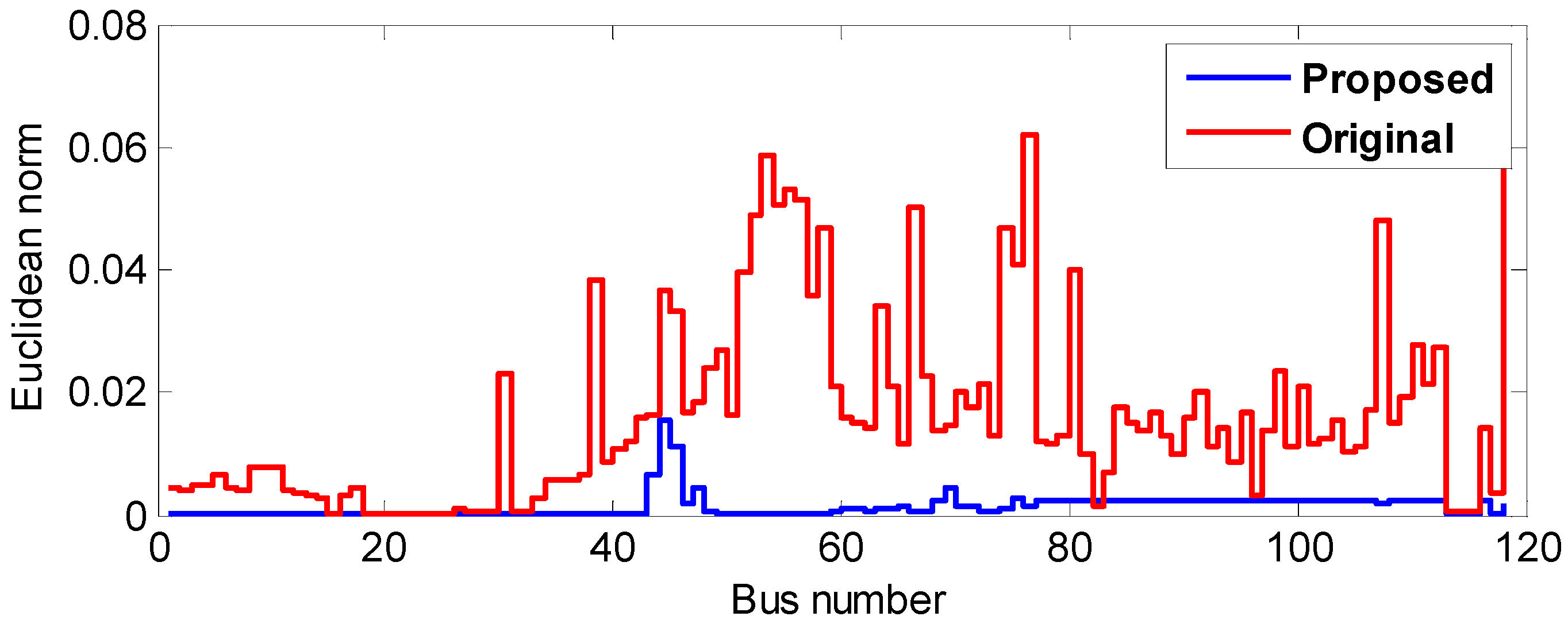
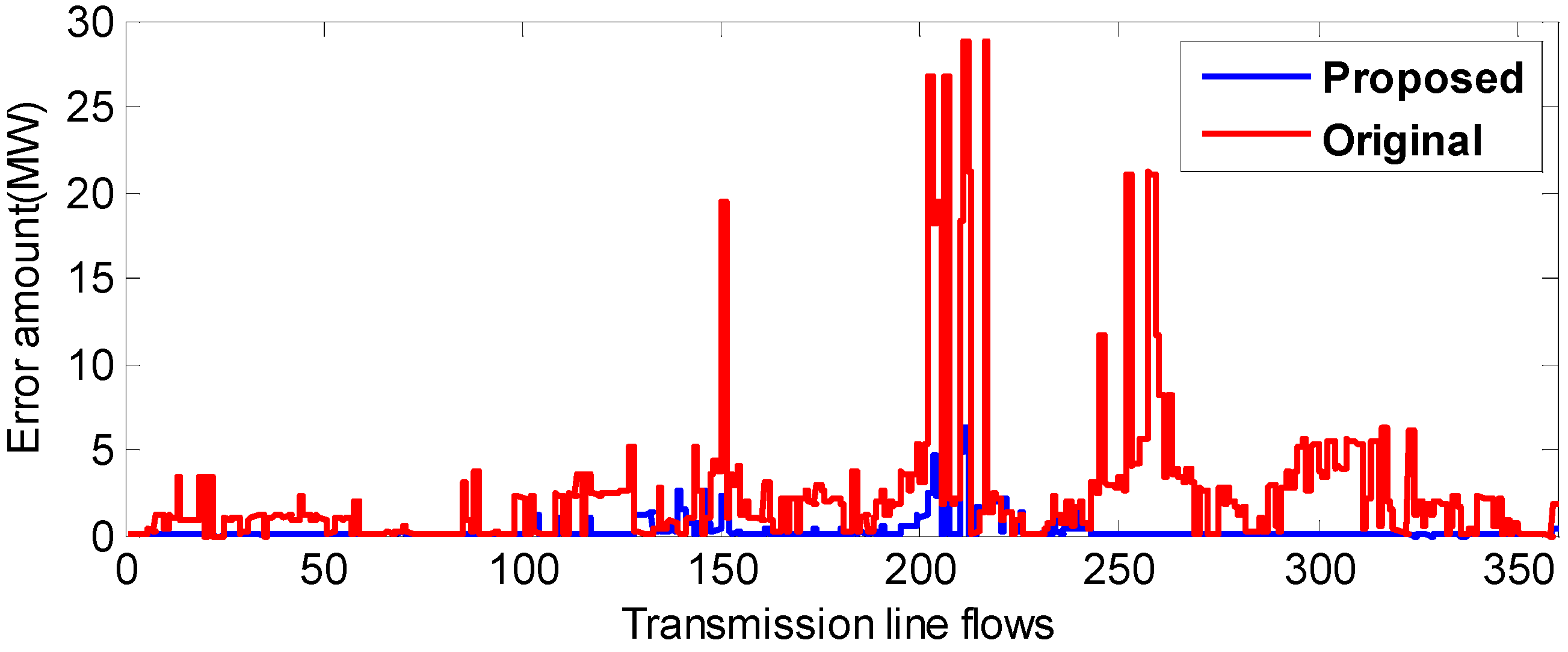
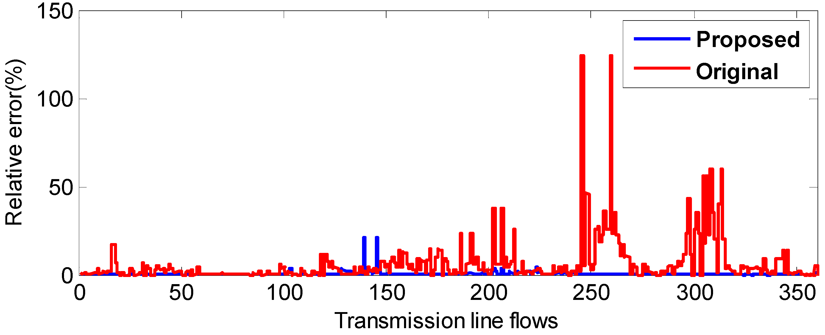
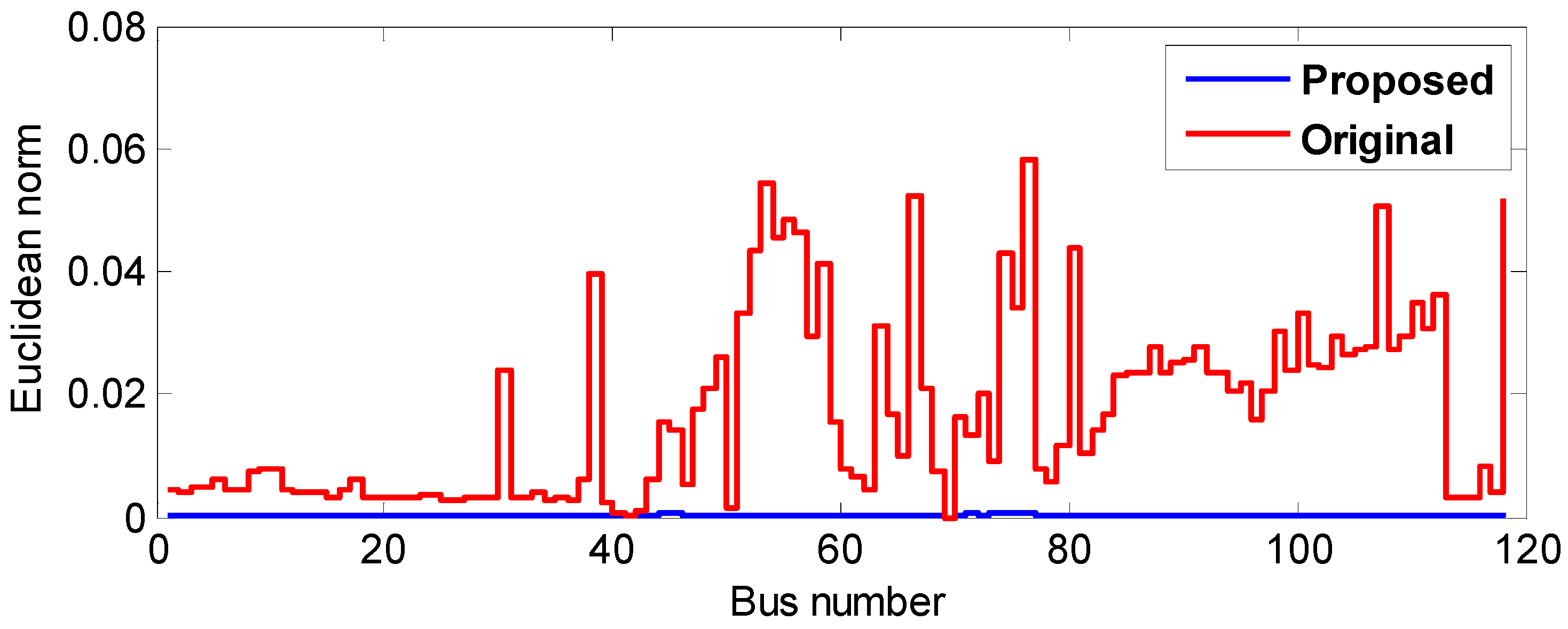
The first simulations are performed with a generator outage (450 MW) at bus 10. The largest generator in the internal system is selected to change the system operating point substantially. The power required to keep the system balanced, after the loss of generation, is picked up by the system slack bus at bus 69. Additional powers from the slack generator are distributed through the network.
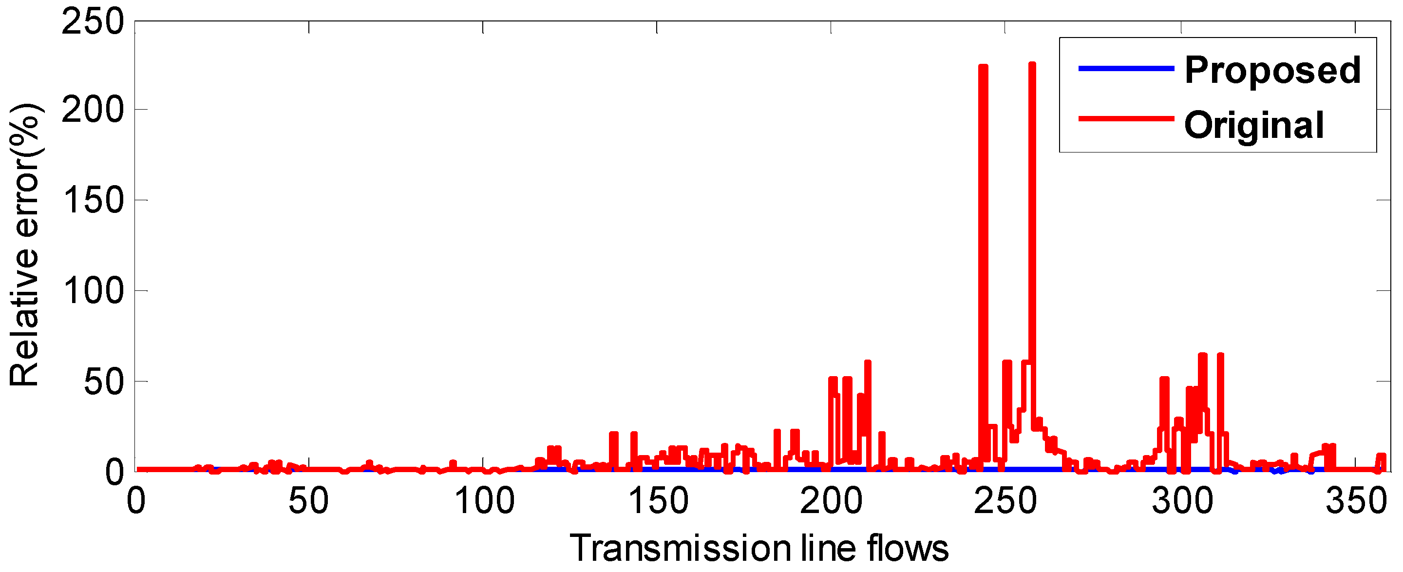
Figure 4 shows the Euclidean norm calculated with the voltage vectors at all system buses. All line power flows in both directions on a transmission line are compared in Figure 5. Relative errors in Figure 6 are calculated only with the line flows larger than 5 MW. As shown in the simulation comparisons, the difference between the ac solution and the proposed approach is much smaller than that between the ac solution and the original mixed approach, for the entire system. In Table 2, the sum of Euclidean norms for the internal system buses is 0.0111 for the proposed approach, while it is 0.2412 for the original mixed approach. The active power flow differences for the entire system are reduced from 844.79 MW with the original approach to 99.05 MW with the proposed approach. The overall simulation accuracy shows an obvious improvement. Moreover, the simulation comparisons show that the proposed method provides better matching in the external system. The improved performance can be understood from the fact that the real power imbalance from the generator outage can be correctly represented with the proposed approach. The original mixed approach has a weakness in the simulation accuracy, and ignoring the real power losses in the conventional dc model has a significant impact on the simulation accuracy.
4.2.2. Line Outage between Buses 23 and 25
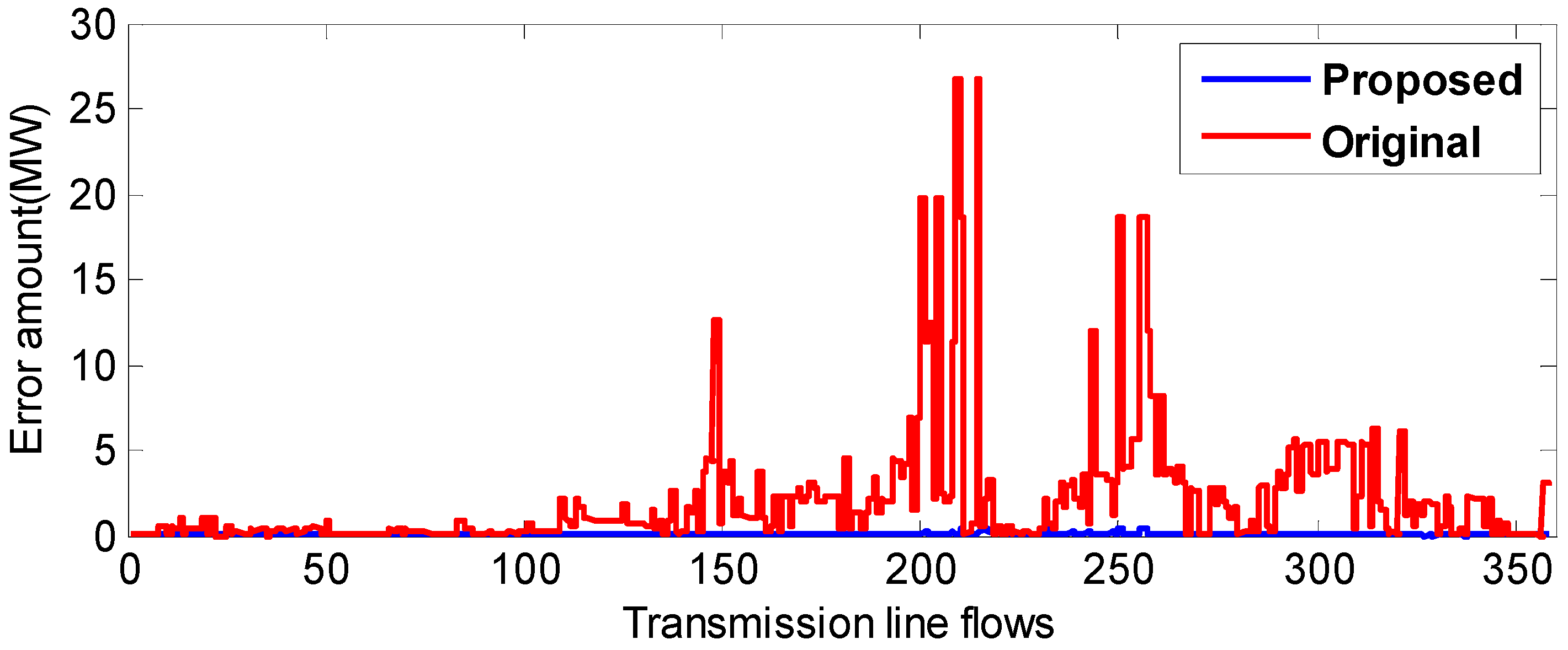
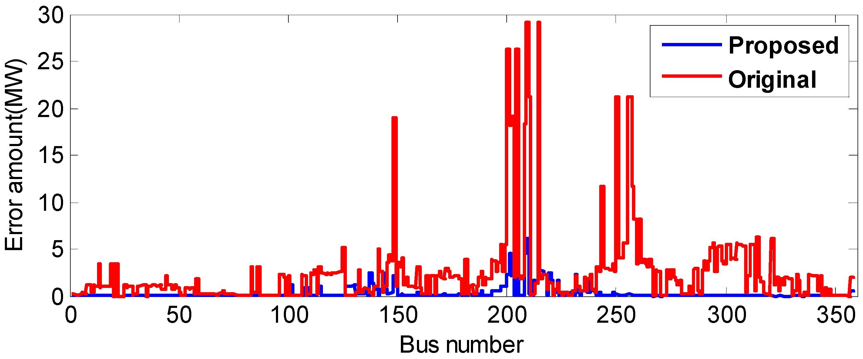
Next, comparisons were made with a transmission line outage in the line connecting buses 23 and 25. For the contingency, one of transmission lines carrying a large amount of real power in the internal system was chosen as the opening line. The transmission line carried approximately 170 MW power. Figure 7, Figure 8 and Figure 9 show the Euclidean distances, errors in the real power flows, and percentage errors of the line flows, respectively. The results in Table 3 show that the errors were reduced from 0.2368 to 0.0035 in the sum of the Euclidean norms, and from 729.99 to 10.07 MW in the real power flows. Although the contingency does not introduce an imbalance in the real powers in the system, the original mixed approach fails to provide good solutions.
4.2.3. Both Contingencies at the Same Time
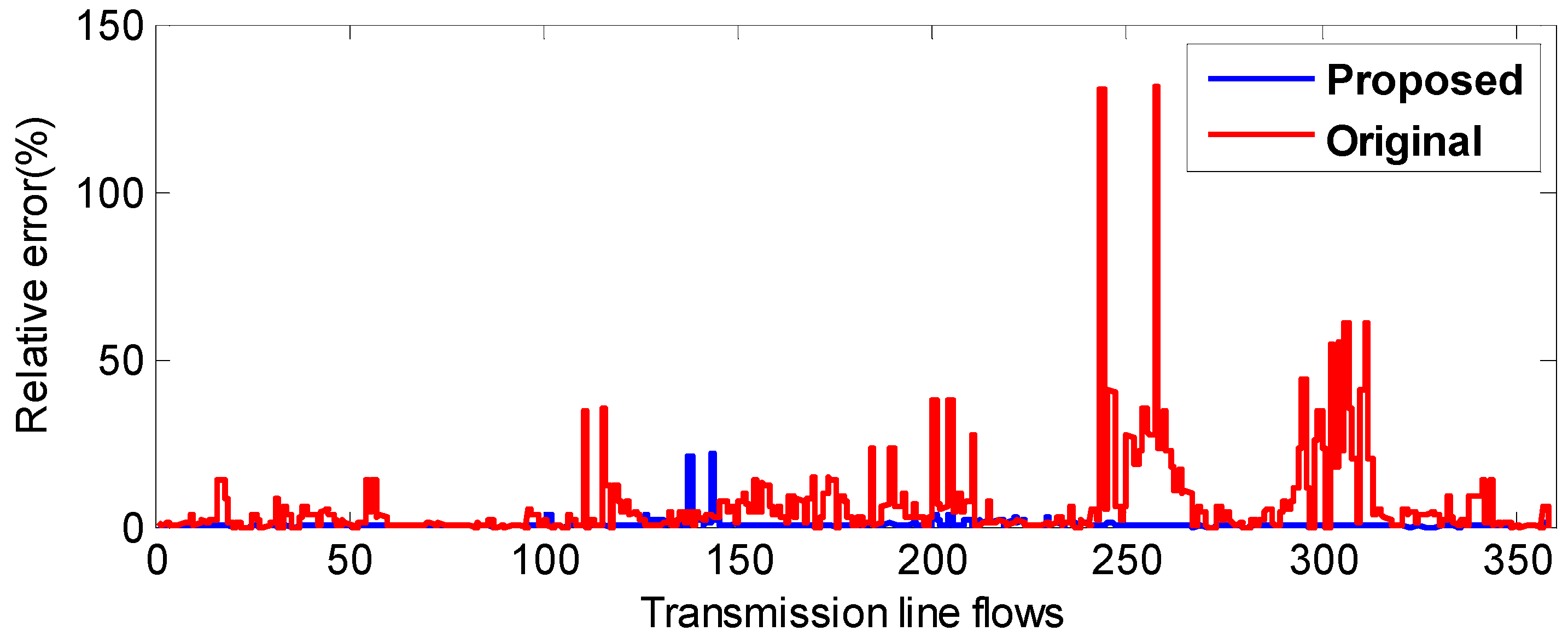
More severe conditions are studied considering the generator and line outages at the same time. Simulation comparisons are shown in Figure 10, Figure 11 and Figure 12. Similar to the previous experiments, the proposed approach provides better simulation accuracy. The simulation results are quite similar to those from the generator outage simulation. It can be inferred that the generator outage introduces more state transitions in the system than the line outage.
The quantified errors depending on the contingency applied are shown in Table 2 and Table 3. Only the internal system buses are considered for the calculation of the sum of the Euclidean norms in Table 2. In Table 3, all real power errors for the entire system are summed up. They prove that the proposed method shows better matching with the ac model solution when compared to the original mixed method.
Comparison of the computation time among three different approaches was made with an Intel Core processor of 3.3 GHz, and the results are listed in Table 4. An average execution time was obtained from 10 simulations. The proposed approach shows 32.5% reduction compared to the full ac method and provides a small increase less than 1% compared with the original method. For the case study, the ratio of the internal to external buses is about 1 to 1.27. More computational benefits are expected with practical systems that have a larger external system.
5. Conclusions
The mixed approach is an extremely attractive power flow analysis model that can speed up the simulation with a simple dc model as well as maintain a high level of simulation accuracy with an accurate ac model. However, the use of the conventional dc model developed with a large amount of simplifications inevitably introduces errors in simulation results. In this paper, an enhanced method is proposed to improve the simulation accuracy of the mixed approach with minor extra computations. The proposed method utilizes the base-case information, which is commonly available, for power system planning, operations, and control. With the available ac solutions, the proposed method modifies the conventional dc model used in the original mixed approach into an advanced model. The new dc model incorporates the real power losses and the voltage magnitude information, which are the most influential factors affecting the accuracy of the dc model. The compensation of real power losses is helpful in preserving the real power balance of the system. The incorporation of voltage magnitude information has an impact on considering the reactive power flows, which are totally neglected in the conventional dc model. Thus, more accurate simulation outcomes can be expected by minimizing the loss of accuracy in the conventional dc model. The superior computational benefits can be retained with a linear formulation of the dc model. The test simulation with the IEEE 118-bus system proved that the proposed approach achieved better simulation accuracy than the original mixed approach, while preserving the advanced computational benefits. The proposed approach can be very useful for applications where accurate and fast simulation outcomes are of great importance.
Author Contributions
Soobae Kim proposed the approach and performed simulation and wrote the paper.
Conflicts of Interest
The author declares no conflict of interest.
References
- Birman, K. Computational Needs for the Next Generation Electric Grid Proceedings; Lawrence Berkeley National Laboratory: Berkeley, CA, USA, 2012. [Google Scholar]
- Stott, B. Review of load-flow calculation methods. Proc. IEEE 1974, 62, 916–929. [Google Scholar] [CrossRef]
- Glover, J.D.; Sarma, M.S.; Overbye, T.J. Power System analysis and Design; Cengage Learning: Stamford, CT, USA, 2012. [Google Scholar]
- Wood, A.J.; Wollenberg, B.F. Power Generation, Operation, and Control; John Wiley & Sons: New York, NY, USA, 1996. [Google Scholar]
- Kaye, R.J.; Wu, F.F. Analysis of Linearized Decoupled Power Flow Approximations for Steady-State Security Assessment. IEEE Trans. Circuits Syst. 1984, 31, 623–636. [Google Scholar] [CrossRef]
- Stott, B.; Alsac, O. Fast Decoupled Load Flow. IEEE Trans. Power Appar. Syst. 1974, 93, 859–869. [Google Scholar] [CrossRef]
- Overbye, T.J.; Cheng, X.; Sun, Y. A comparison of the AC and DC power flow models for LMP calculations. In Proceedings of the 37th Annual Hawaii International Conference on System Sciences, Big Island, HI, USA, 5–8 January 2004.
- Purchala, K.; Meeus, L.; Van Dommelen, D.; Belmans, R. Usefulness of DC power flow for active power flow analysis. In Proceedings of the 2005 IEEE Power Engineering Society General Meeting, San Francisco, CA, USA, 12–16 June 2005.
- Hertein, D.V.H.; Verboomen, J.; Purchala, K.; Belmans, R.; Kling, W.L. Usefulness of DC power flow for active power flow analysis with flow controlling devices. In Proceedings of the 8th IEE International Conference on AC-DC Power Transmission (ACDC 2006), London, UK, 28–31 March 2006.
- Stott, B.; Jardim, J.; Alsac, O. DC Power Flow Revisited. IEEE Trans. Power Syst. 2009, 24, 1290–1300. [Google Scholar] [CrossRef]
- Qi, Y.; Shi, D.; Tylavsky, D. Impact of assumptions on DC power flow model accuracy. In Proceedings of the 2012 North American Power Symposium (NAPS 2012), Champaign, IL, USA, 9–11 September 2012.
- Fatemi, S.; Abedi, S.; Gharehpetial, G.B.; Hosseinian, S.H.; Abedi, M. Introducing a Novel DC Power Flow Method with Reactive Power Considerations. IEEE Trans. Power Sys. 2015, 30, 3012–3023. [Google Scholar] [CrossRef]
- Kim, S.; Overbye, T.J. Mixed power flow analysis using AC and DC models. IET Gener. Transmi. Distrib. 2012, 6, 1053–1059. [Google Scholar] [CrossRef]
- Abur, A.; Exposito, A.G. Power System State Estimation: Theory and Implementation; CRC press: Boca Raton, FL, USA, 2012. [Google Scholar]
- Monticelli, A. State Estimation in Electric Power Systems: A Generalized Approach; Springer Science & Business Media: Berlin, Germany, 1999. [Google Scholar]
- Lu, S.; Zhou, N.; Kumar, N.P.; Samaan, N.; Chakrabarti, B.B. Improved DC power flow method based on empirical knowledge of the system. In Proceedings of the 2010 IEEE/PES Transmission and Distribution Conference and Exposition, New Orleans, LA, USA, 19–22 April 2010.
- University of Washington Power Systems Test Case Archive. Available online: https://www.ee.washington.edu/research/pstca (accessed on 20 September 2016).
Figure 1.
Procedure of the mixed power flow method.
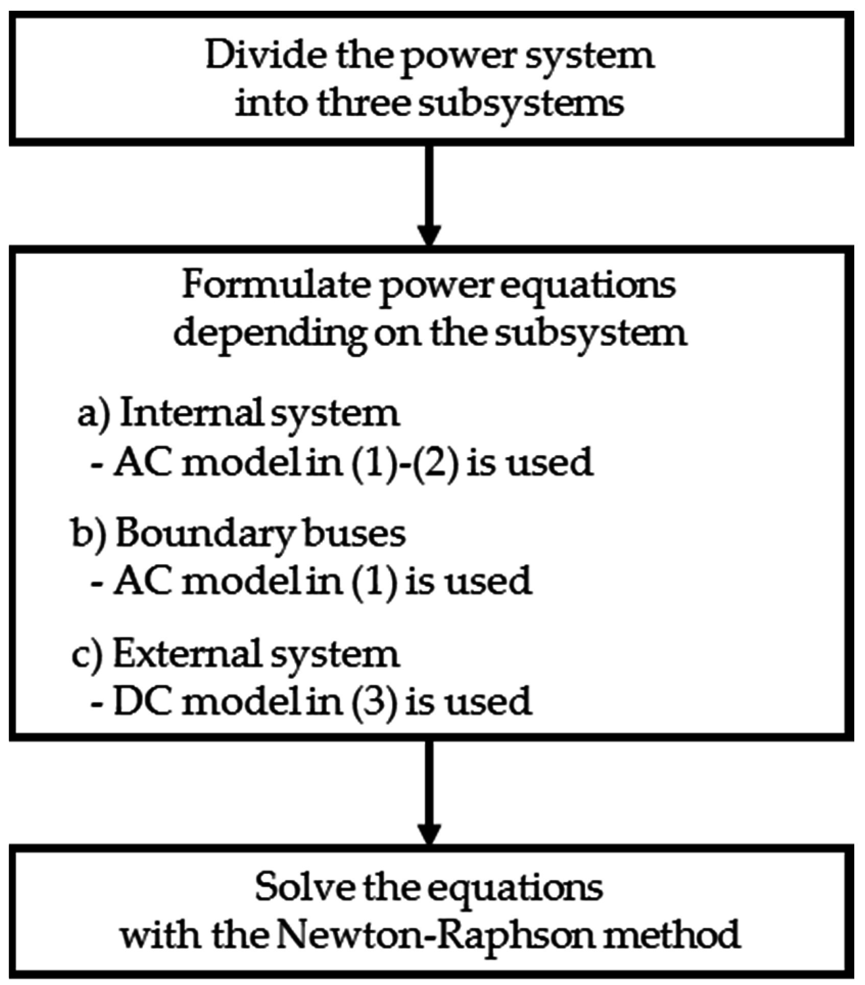
Figure 2.
Procedure of the proposed approach.
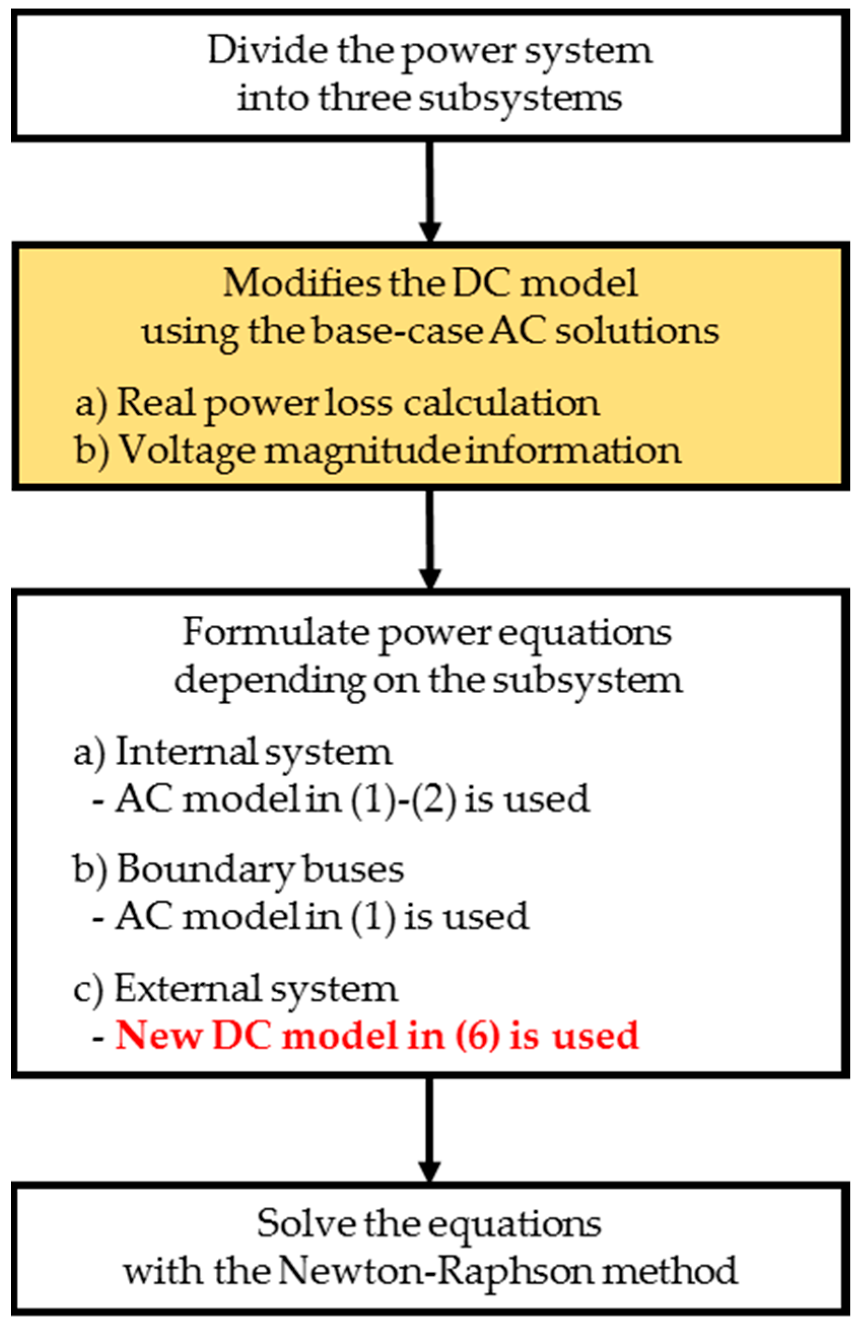
Figure 3.
IEEE 118-bus system [17].
Figure 3.
IEEE 118-bus system [17].
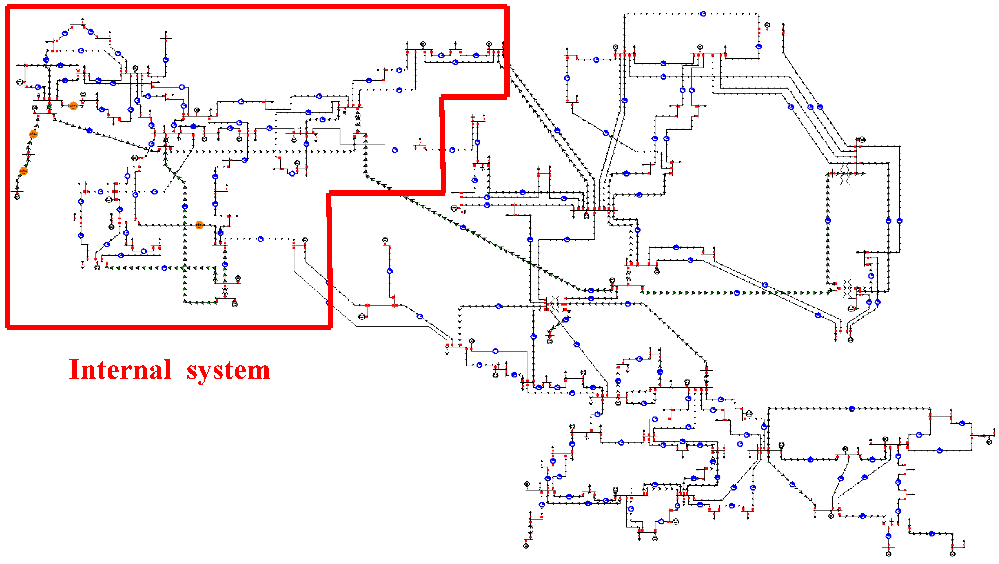
Figure 4.
Euclidean norm with the generator outage (450 MW) at bus 10.

Figure 5.
Errors in the real power with the generator outage (450 MW) at bus 10.

Figure 6.
Relative errors in the real power with the generator outage (450 MW) at bus 10.

Figure 7.
Euclidean norm with the line outage.

Figure 8.
Errors in the real power with the line outage.

Figure 9.
Relative errors in the real power with the line outage.

Figure 10.
Euclidean norm with both contingencies.

Figure 11.
Errors in the real power with both contingencies.

Figure 12.
Relative errors in the real power with both contingencies.


| Internal System Buses | Boundary Buses | |
|---|---|---|
| Test system | 1~43, 113, 114, 115, 117 (47 buses) | 44, 49, 65, 70, 72 |
| Contingecy | Proposed Approach (A) | Original Method (B) | Comparison Between Two Methods (=A/B × 100%) |
|---|---|---|---|
| Generator outage | 0.0111 | 0.2412 | 4.60% |
| Line outage | 0.0035 | 0.2368 | 1.48% |
| Both contingencies | 0.0102 | 0.2394 | 4.26% |
| Contingency | Proposed Approach | Original Method |
|---|---|---|
| Generator outage | 99.05 | 844.79 |
| Line outage | 10.07 | 729.99 |
| Both contingencies | 98.142 | 842.71 |
| Full AC | Proposed Approach | Original Method | |
|---|---|---|---|
| Time (s) | 1.60 | 1.08 | 1.07 |
| Percentage Ratio (%) | 100% | 67.5% | 66.9% |
© 2016 by the author; licensee MDPI, Basel, Switzerland. This article is an open access article distributed under the terms and conditions of the Creative Commons Attribution (CC-BY) license (http://creativecommons.org/licenses/by/4.0/).
Share and Cite
MDPI and ACS Style
Kim, S. Accuracy Enhancement of Mixed Power Flow Analysis Using a Modified DC Model. Energies 2016, 9, 776. https://doi.org/10.3390/en9100776
AMA Style
Kim S. Accuracy Enhancement of Mixed Power Flow Analysis Using a Modified DC Model. Energies. 2016; 9(10):776. https://doi.org/10.3390/en9100776
Chicago/Turabian StyleKim, Soobae. 2016. "Accuracy Enhancement of Mixed Power Flow Analysis Using a Modified DC Model" Energies 9, no. 10: 776. https://doi.org/10.3390/en9100776
Note that from the first issue of 2016, this journal uses article numbers instead of page numbers. See further details here.