A Permutation Importance-Based Feature Selection Method for Short-Term Electricity Load Forecasting Using Random Forest

Abstract

The prediction accuracy of short-term load forecast (STLF) depends on prediction model choice and feature selection result. In this paper, a novel random forest (RF)-based feature selection method for STLF is proposed. First, 243 related features were extracted from historical load data and the time information of prediction points to form the original feature set. Subsequently, the original feature set was used to train an RF as the original model. After the training process, the prediction error of the original model on the test set was recorded and the permutation importance (PI) value of each feature was obtained. Then, an improved sequential backward search method was used to select the optimal forecasting feature subset based on the PI value of each feature. Finally, the optimal forecasting feature subset was used to train a new RF model as the final prediction model. Experiments showed that the prediction accuracy of RF trained by the optimal forecasting feature subset was higher than that of the original model and comparative models based on support vector regression and artificial neural network.

1. Introduction

Load forecast (LF) is the basis for the planning, operating, and scheduling of traditional power networks. LF is also the basis for creating an efficient power system by reducing operational costs and using the renewable energy source of the smart grid [1]. LF can be divided into three categories according to forecast horizon: long-term LF, mid-term LF, and short-term LF (STLF) [2]. STLF generally refers to the prediction of load one hour, one day, or one week ahead [3]. The prediction accuracy of STLF is directly related to the safety, stability, and economy of power system operation. Considering an electrical utility in the United Kingdom as an example, a decrease of 1% in prediction error can result in a decrease of approximately 10 million pounds in operational costs [4]. Therefore, in the smart grid and deregulated power market environment, power systems require high prediction accuracy of STLF.

STLF methods are divided into traditional and artificial intelligence methods. The traditional methods mainly include Kalman filtering [5], exponential smoothing [6], regression analysis [7], and autoregressive integrated moving average (ARIMA) methods [8,9]. These methods have simple principles and mature technologies, but lack self-learning capability and have difficulty describing complex non-linear models accurately [10]. The artificial intelligence methods mainly include the fuzzy logic (FL) method [11,12], the artificial neural network (ANN) [13,14,15], support vector regression (SVR) [16,17,18], and random forest (RF) [19,20,21]. The FL method has strong adaptability and can deal with fuzzy phenomena in power systems. However, FL can only roughly map the output and has weak learning capability. ANN has been extensively used in the field of STLF because of its excellent self-learning and fault-tolerant capabilities. Nevertheless, ANN easily falls to overfitting and local optimum. A unified approach for choosing the network structure and connection weights is also lacking [16], thereby resulting in several errors and instabilities for the application of ANN to STLF. SVR follows the structural risk minimization principle to improve the generalization capability, a principle different from that of empirical risk minimization of ANN. Therefore, SVR overcomes the numerous disadvantages of ANN [22]. However, when constructing the forecast model, the structure and parameters of SVR must be adjusted according to different inputs. The optimization process is relatively complex. Unlike other methods, RF is an artificial intelligence method that combines decision tree (DT) and integrated algorithm together. RF has the advantages of good anti-noise capability and strong resistant to overfitting. Only a few parameters of RF need to be optimized as compared with other methods [23].

The feature set used as the input of these artificial intelligence forecast methods can directly affect the prediction accuracy and efficiency of the forecasting model [24,25,26]. Electrical LF refers to the accurate prediction of future electric power load based on a large quantity of historical load data and other related factors. Therefore, the present study aims to obtain the optimal feature subset for the forecasting model through feature selection methods. However, most artificial intelligence forecast methods cannot conduct the feature selection process and need to be combined with another feature selection algorithm to do so. Che et al. combined SVR with an approximation convexity optimization framework with three different initial values of the optimal feature subset dimension m converged to the same value at the stop condition to obtain the optimal feature subset [24]. Ghofrani et al. and Kouhi et al. combined ANN and correlation analysis [25,26]. By calculating the correlation coefficient of model input and output, the relevant features are retained and the redundant features are eliminated. Although the above studies have made progress in the feature selection of STLF, the constantly changing input feature subsets used in the process of feature selection require the adjustment and optimization of forecasting model parameters. Furthermore, forecasting models have difficulty achieving optimal forecasting results, and the optimal feature subset needs to be evaluated by the prediction error of the forecasting model. SVR and ANN have difficulty obtaining the minimum prediction error of different feature subsets, thus affecting the feature selection result.

When the original feature set is used to train an RF model, the permutation importance (PI) value of each feature for prediction can be obtained in the training process. On this basis, the optimal features can be selected through the sequential backward search (SBS) method. Thus, when used for load forecasting, RF need not be combined with complex feature selection algorithms. Furthermore, if the number of DTs in RF is sufficiently large, then only one parameter needs to be adjusted when the feature subset dimension changes. This parameter can be conveniently calculated using the empirical formula. Unlike SVR and ANN, RF is more suitable for feature selection of STLF. Determining the threshold for feature selection methods and modifying the numerous parameters of the predictor according to the different feature subsets are difficult. However, the optimal feature subset can be easily selected by combining PI with the improved SBS strategy. Consequently, the abovementioned shortcomings can be overcome and the accuracy of STLF can be improved.

In this paper, a novel RF-based feature selection method for STLF is proposed. First, 243 related features are extracted from historical load data and time information of predicted point to form the original feature set. The load data for a full year are divided into a training set and a test set by random sampling. Subsequently, the original feature set is used to train an RF as the original model. After the training process, the prediction error of the original model on the test set is recorded as the threshold to evaluate the forecasting capability of different feature subsets and obtain the PI value of each feature. Then, the improved SBS method is used to select the optimal forecasting feature subset according to the PI value of each feature. Finally, the optimal forecasting feature subset is used to train a new RF as the final prediction model. The historical load data for 2012 of a city in Northeast China are used for comparative experiments and to demonstrate the superiority of the proposed method in feature selection and load forecasting.

The rest of the paper is organized as follows. Section 2 introduces RF, and Section 3 describes the RF learning process and the proposed feature selection method. Section 4 presents the real load data for experiments, and analyzes and discusses the feature selection and STLF results. Finally, Section 5 elaborates the conclusions and future work.

2. Mathematical Preliminaries

RF is an intelligent algorithm that combines DT with integrated algorithm. RF not only possesses the numerous advantages of DT, but also overcomes the poor generalization capability of DT. As compared with DT, RF enhances the precision of classification and regression without significantly increasing its computational complexity.

2.1. Decision Tree

DT is a type of classical machine learning algorithm. As an example of DT models, classification and regression tree (CART) can be used for classification and regression analysis [27,28]. DT is an inverted tree. The top of DT is the root node, which contains all the training samples. The optimal feature is selected from the original feature space to split each of the non-leaf nodes in DT until the stop condition is reached. If all the samples contained in a node belong to one class, then this node is defined as a leaf node. Splitting the leaf node is unnecessary, and each path connecting the root node and the leaf node represents a partition rule.

DT has a simple principle and structure and can thus be constructed easily with high efficiency. Although DT can explain the training set perfectly, its dependency on the training samples increases when grown freely. Accordingly, the generalization capability of DT weakens, thereby lowering its resistance to overfitting. Therefore, a pruning operation must be conducted to restrict the free growth of DT. DT may also fall into the local optimal state, thereby weakening the explanation capability of the single DT.

2.2. Random Forest

RF was proposed by Breiman in 2001 [23] to overcome the shortcomings of DT. RF combines CART and the bagging algorithm and builds a new DT set based on ensemble learning methods.

$$\left\{t(x,s_{{\mathsf{\Theta }}_1}),t(x,s_{{\mathsf{\Theta }}_2}),\dots ,t(x,s_{{\mathsf{\Theta }}_m})\right\},$$

(1)

where $t(x,s_{{\mathsf{\Theta }}_k})$ is the base classifier, which represents a CART ($k=1,2,\dots ,m$); x is the input vector of CART; and $s_{{\mathsf{\Theta }}_k}$ is a random vector, which determines the random extraction process of training samples for the kth tree. The growth process of the kth tree is also determined by $s_{{\Theta }_k}$. Meanwhile, all $s_{{\mathsf{\Theta }}_k}$ values are independent of one another but share the same distribution.

For integrated algorithms, the difference of base classifiers can significantly affect their performance [29]. The two methods of RF randomness described below ensure significant difference among the base classifiers.

• Assume S is the original sample set with n samples. When bagging is used to generate the training set for each CART, each of the samples in the original sample space has $1/n$ probability to be selected. Based on the characteristics of bagging, several samples may never be selected, whereas other samples may be selected more than once. All samples that have never been selected are the out-of-bag (OOB) dataset of this tree. Therefore, the training set of each CART is different, thus reducing the correlation between the trees in RF. The diversity of CART increases the capability of RF to resist noise and reduces its sensitivity to outliers. These are the main advantages that bagging brings to RF.
• RF differs from DT in terms of selecting a feature to split a non-leaf node. Specifically, instead of searching the entire original feature space M to select the best feature, RF randomly generates a candidate segmentation feature set m for each non-leaf node. The set m is a subset of the original feature set with $m_{try}$ features ($m_{try}$ is no longer changed once determined). Thereafter, the optimal feature is selected from m to split this node.

The two ways of RF randomness make its CARTs different from one another. Thus, RF has a wide range of applications and requires few parameters to be adjusted and optimized. Only two parameters can affect the forecasting performance of RF, that is, the tree number $n_{tree}$ and the dimension $m_{try}$ of the candidate segmentation feature set. When the number of trees in RF is low, the performance of RF is very poor and its precision fails to meet the requirements of regression prediction. According to the Strong Law of Large Numbers and the tree structure, the generalization error of RF will tend to be a stable upper bound with the rise in tree number [23]. As a result, RF becomes resistant to overfitting. Compared with that of $n_{tree}$, $m_{try}$ has a larger effect on the performance of RF. After considerable experimental research, the default experience value for $m_{try}$ when RF is used for regression has been obtained [21]:

$$m_{try}=\frac{t}{3}.$$

(2)

In this equation, t represents the dimension of the original feature set.

RF can provide two kinds of useful indices, namely OOB error and the importance value of each feature, after completing the training process. According to the characteristics of bagging, approximately one-third of the samples in the original sample space will never be selected when the training set is generated for each tree. Therefore, for each sample j, approximately one-third of trees exist in RF that are not contained in this sample. These trees are then used to predict sample j. The OOB error is calculated by:

$$OOBError=\frac{1}{n}{\displaystyle \sum _{i=1}^n{\left(y_r-y_p\right)}^2},$$

(3)

where n represents the number of all samples, $y_r$ is the true value of sample i, and $y_p$ is the predictive value of sample i. The OOB error can be used to estimate the generalization error of RF. Meanwhile, the PI value of each feature can be calculated based on the OOB dataset, which can significantly benefit the following feature selection stage.

After the training process, the final predictive result can be obtained by averaging the output of all trees:

$$y=\frac{1}{c}{\displaystyle \sum _{i=1}^c{y}_i}.$$

(4)

In this equation, $c=n_{tree}$ represents the number of trees in RF and $y_i$ is the predictive value of the ith tree.

3. Random Forest (RF) Learning Process and Feature Selection for Short-Term Load Forecast (STLF)

In the STLF field, a large number of features must be considered, such as historical load data and hourly and daily information. If all the features are used for load forecasting, then the prediction accuracy and efficiency of the forecasting model can decrease because of the existence of redundant features. Thus, the optimal feature subset must be constructed by removing the redundant features. In the early stage, the feature subset is artificially specified by expert experience. However, this process is unreasonable and less credible. In the current load forecasting field, the feature selection methods are necessary to optimize numerous parameters for every feature subset. As a result, the feature selection becomes time-consuming and the error caused by the unreasonable design of the parameters cannot be avoided easily. RF can guarantee the optimization of the model by adjusting only a small number of parameters. After completing the training process, RF can provide the importance value of each feature for prediction. The redundant features can then be removed step by step according to the importance value. Accordingly, the feature selection process of STLF can be significantly simplified.

3.1. RF Learning Strategy

RF is a collection of numerous DTs. Therefore, RF has a simple structure with strong anti-noise capability and can overcome the interpretation capability disadvantage of a single DT. The Strong Law of Large Numbers guarantees that RF will nearly never fall to overfitting. Its numerous advantages make RF suitable for application in power system load forecasting [19].

By obtaining the historical load data and hourly and daily information, the original sample space with dimension n is constructed. On this basis, n samples are randomly selected with replacement from the original sample space according to the bagging principle. The selected samples form a new training set for the CART. The rest of the samples form the OOB dataset of this tree. The process is repeated for $n_{tree}$ times. These $n_{tree}$ training sets are then used to construct $n_{tree}$ CARTs. All the trees grow freely without pruning operation.

When a non-leaf node is split, the segmentation effect of a feature is determined by Gini index. Assuming that a non-leaf node A contains the dataset D, a total of d samples exist in D. The Gini index of set D before being split by a feature is as follows:

$$Gin{i}_{before}(D)=1-{\displaystyle \sum _{j=1}^l{\left(\frac{d_j}{D}\right)}^2},$$

(5)

where l represents the number of categories contained in D; and $d_j(j=1,2,\dots ,l)$ is the set composed of the samples belonging to the jth class. If feature F is used to split node A, then D is divided into o subsets $(D_1,D_2,\dots ,D_o)$. A total of $d_i$ samples exist in set $D_i$ $(i=1,2,\dots ,o)$. Accordingly, the Gini index of set D after segmentation is:

$$Gin{i}_{after}\left(D\right)=\frac{d_1}{d}Gin{i}_{before}(D_1)+\cdots +\frac{d_o}{d}Gin{i}_{before}(D_o).$$

(6)

According to Equation (6), the Gini index is inversely proportional to the segmentation effect. Therefore, the feature with smaller $Gin{i}_{after}$ can achieve better performance.

3.2. Feature Selection for Load Forecasting Based on Permutation Importance (PI) and Optimal SBS Method

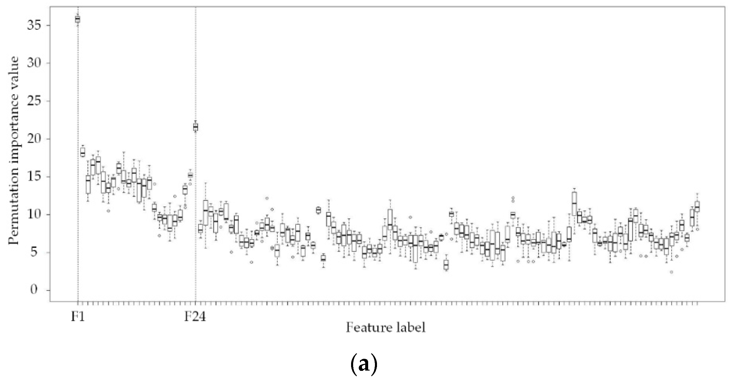
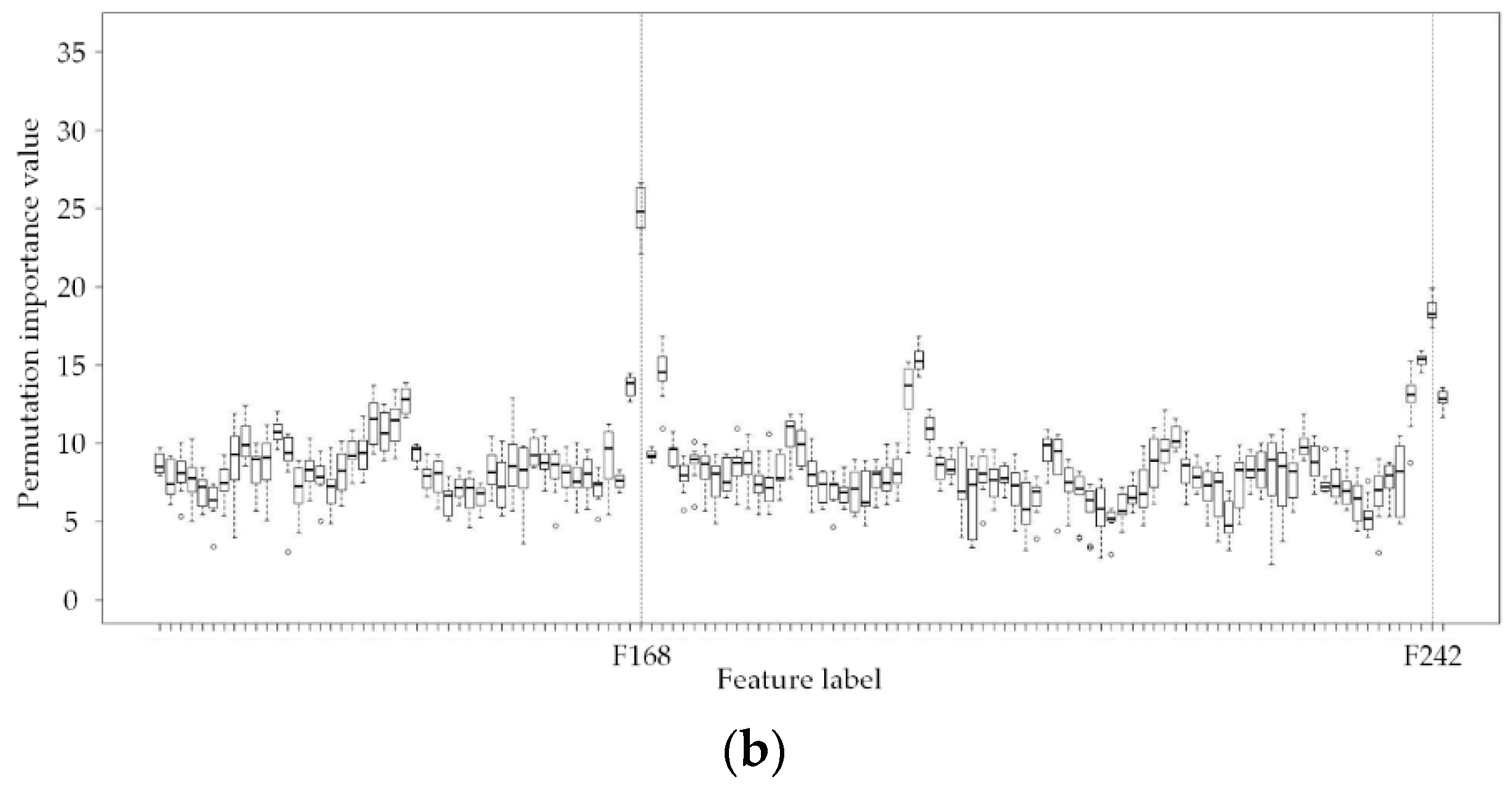
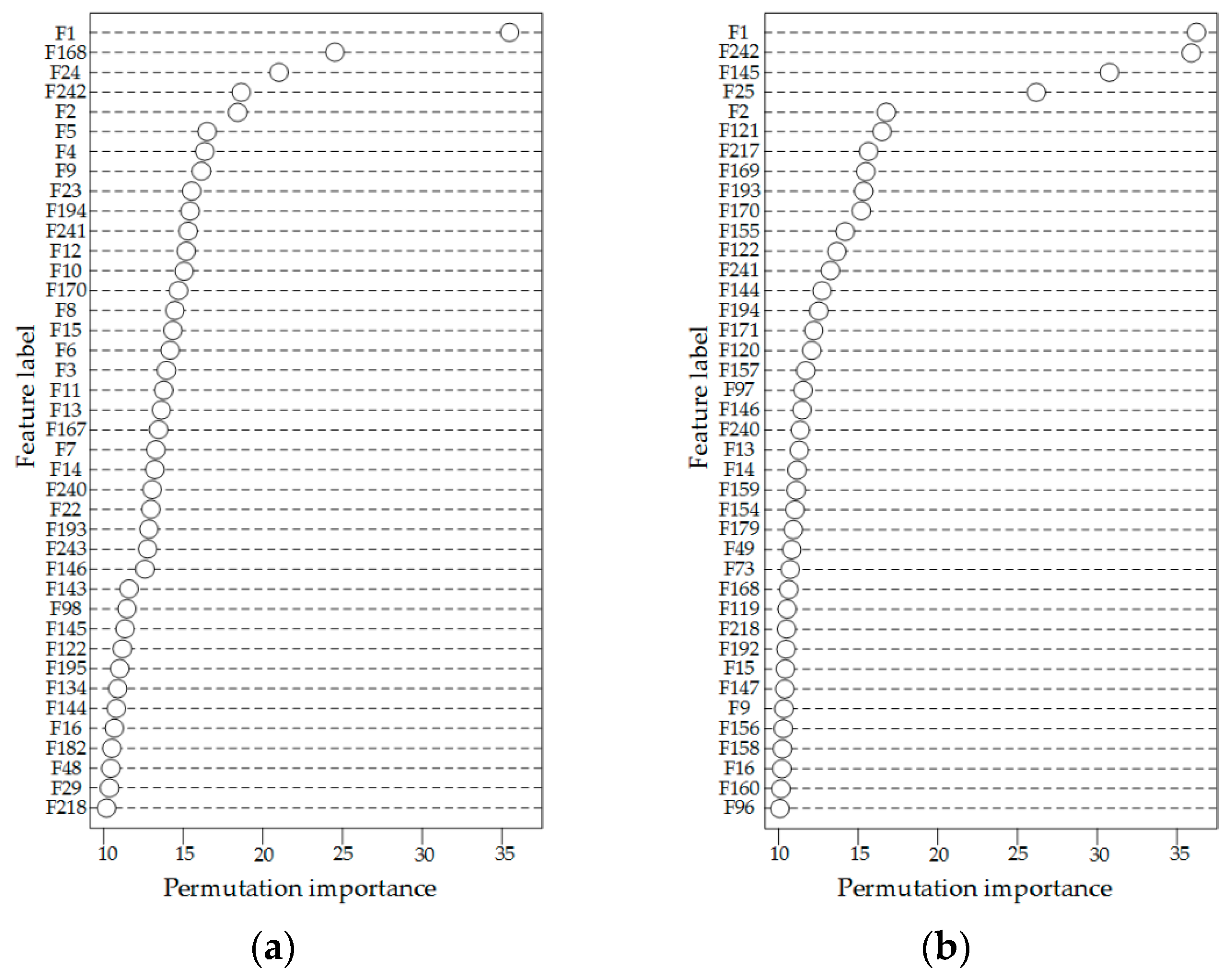
3.2.1. Feature Importance Analysis Based on Permutation Importance (PI)

RF can determine the importance of a feature to STLF by calculating the PI value of each feature. When calculating the importance value of feature $F^j$ based on the ith tree, $OOBErro{r}_i$ is first calculated based on Equation (3). Then, the values of feature $F^j$ in the OOB dataset are randomly rearranged and those of the other features are unchanged, thereby forming a new OOB dataset $OO{B_i}^{\prime }$. With the new $OO{B_i}^{\prime }$ set, $OOBErro{r_i}^{\prime }$ can also be calculated using Equation (3). The PI value of feature $F^j$ based on the ith tree can be obtained by subtracting $OOBErro{r}_i$ from $OOBErro{r_i}^{\prime }$.

$$P{I}_i\left(F^j\right)=OOBErro{r_i}^{\prime }-OOBErro{r}_i,$$

(7)

The calculation process is repeated for each tree. The final PI value of feature $F^j$ can be obtained by averaging the PI values of each tree:

$$PI\left(F^j\right)=\frac{1}{c}{\displaystyle \sum _{i=1}^{c}P{I}_i\left(F^j\right)},$$

(8)

where $c=n_{tree}$ represents the tree number. If a feature is important, then its values of different samples will be dissimilar. After the values of this feature are randomly rearranged on the OOB dataset, the discrimination of different samples will be reduced. The feature with high PI value is more important than the other features.

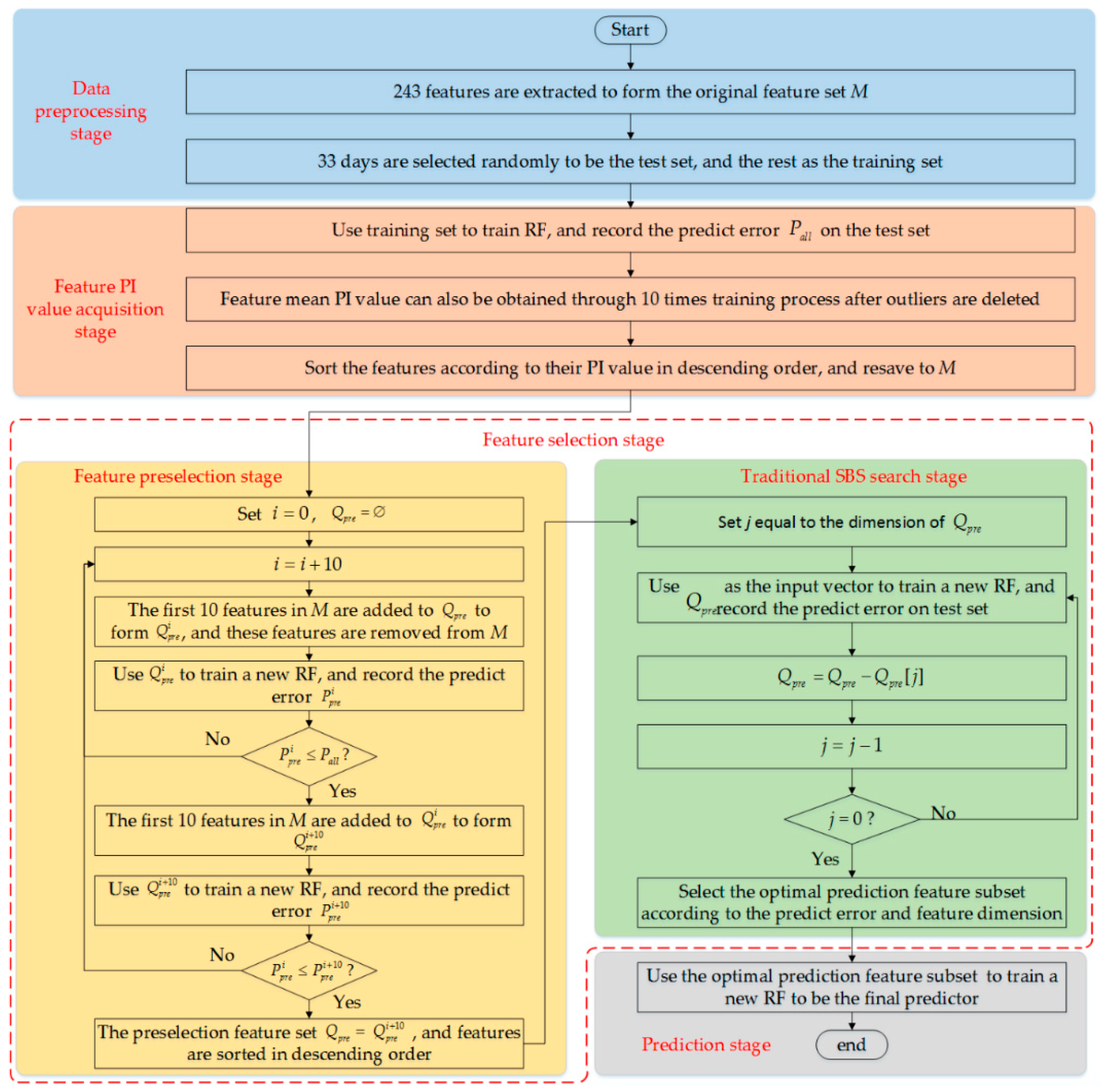
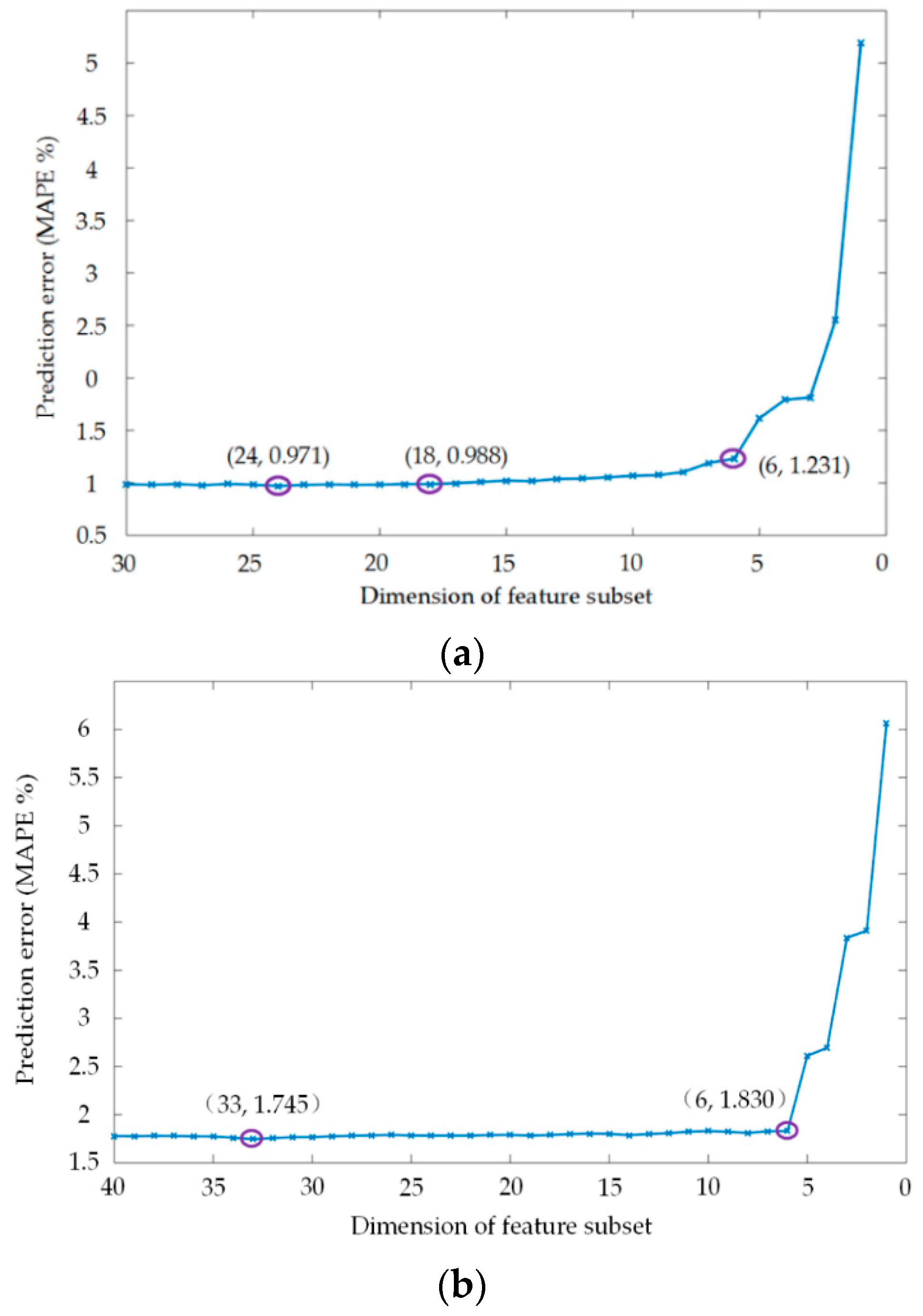
3.2.2. Optimal Sequential Backward Search (SBS) Method for Feature Selection of Short-Term Load Forecast (STLF)

On the basis of the PI value of all the features combined with the SBS method, the optimal feature subset can be determined. However, considering that the dimension of the original load feature set is relatively high, the process of feature selection will be time-consuming when using the SBS method. Thus, an improved SBS method is proposed.

A preselection stage is added before using the traditional SBS method. The steps of the preselection stage are described as follows.

• The original load feature set is used as the input to train an RF. After the training process is completed, the test set is used to evaluate the performance of this RF. Thereafter, the prediction error $P_{all}$ can be obtained and set as a threshold value. The PI value of each feature can also be obtained.
• According to the PI value, all features are rearranged in a descending order and are resaved to the original feature set M.
• The first 10 features with the highest PI value are added to the preselection feature set $Q_{pre}$, which is an empty set at first. Subsequently, these features are removed from set M.
• Let set $Q_{pre}^i$ (superscript i represents the number of features in the set) be equal to set $Q_{pre}$. Set $Q_{pre}^i$ is then used to retrain a new RF and the prediction error is recorded as $P_{pre}^i$.
• If $P_{pre}^i\le P_{all}$, then the first 10 features of set M are added to set $Q_{pre}^i$ to form the set $Q_{pre}^{i+10}$. The training and testing processes are repeated using set $Q_{pre}^{i+10}$.
• If $P_{pre}^{i+10}\ge P_{pre}^i$, then adding another feature to set $Q_{pre}$ is unnecessary. Otherwise, the first 10 features of set M must be added to set $Q_{pre}$ and must be removed from set M. This condition indicates that the stop conditions are $P_{pre}^i\le P_{all}$ and $P_{pre}^{i+10}\ge P_{pre}^i$.
• The preceding steps are repeated until the stop condition is met or set M is empty.
• The preselection feature set $Q_{pre}$ is obtained and is equal to set $Q_{pre}^i$, and the preselection stage ends.

After determining the preselection feature set $Q_{pre}$, the traditional SBS method is applied to set $Q_{pre}$. The features in set $Q_{pre}$ are removed one by one, from smallest to largest according to their PI values, until set $Q_{pre}$ is empty. Whenever a feature is removed, set $Q_{pre}$ is used to retrain a new RF and the prediction error on the test set is recorded. The optimal forecasting feature subset $Q_{best}$ is obtained by considering prediction error and feature set dimension. The flowchart of the algorithm is shown in Figure 1.

Unlike the traditional SBS method, a preselection stage is added in the method proposed in this paper. By spending a small amount of time, a preselection feature set $Q_{pre}$ that is much smaller than the original feature set M can be obtained. On this basis, the traditional SBS method is performed within a relatively small amount of time. Therefore, the proposed algorithm is very suitable for load forecasting with high dimensional feature sets.

4. Experimental Results and Analysis

The data used in the experiment are all real historical load data. Two kinds of error evaluation criteria, namely, mean absolute percentage error (MAPE) and root mean square error (RMSE), are used to evaluate the load forecasting results. The calculation formula of MAPE and RMSE are described in Equations (9) and (10):

$$MAPE=\frac{1}{n}{\displaystyle \sum _{t=1}^n\frac{\left|y_r(t)-y_p(t)\right|}{y_r(t)}}\times 100\%,$$

(9)

$$RMSE=\sqrt{\frac{{\displaystyle \sum _{t=1}^n{\left(y_r(t)-y_p(t)\right)}^2}}{n}},$$

(10)

where n represents the number of sample points, $y_r(t)$ is the real load value of hour t, and $y_p(t)$ is the forecasting load value of hour t.

4.1. Dataset

The historical load data for 2012 of a city in the northeast of China are used for the experiment. This historical load dataset contains a total of 366 days. According to Jurado et al., a total of 9% of these days (33 days) are randomly selected as the test set, and the remaining 91% (333 days) are used as the training set [20]. When the load data are sampled in this city, the sampling is 1 h. The load curve of the entire year is shown in Figure 2.

Figure 2 clearly shows three huge falls in the curve. These three falls correspond to the three main holidays of this year, that is, the Spring Festival, the Labor Day holiday, and National Day. The load consumed in the winter gradually increases because of the cold weather.

The entire year is divided into a training set and a test set by random sampling. To increase the reliability of the experiment, 33 days of the test set are randomly and equally distributed in four quarters (approximately eight days per quarter). The relevant information for each day of the test set is listed in

Table 1. The relevant information for each day of the test set.

The First Quarter (1/1/2012 to 31/3/2012)	The Second Quarter (1/4/2012 to 30/6/2012)	The Third Quarter (1/7/2012 to 30/90/2012)	The Fourth Quarter (1/10/2012 to 31/12/2012)
5 and 8/1/2012 (Thur., Sun.) 4, 9 and 24/2/2012 (Sat., Thur., Fri.) 3, 23 and 31/3/2012 (Sat., Fri., Sat.)	1 and 20/4/2012 (Sun., Fri.) 10, 18, 25 and 31/5/2012 (Thur., Fri., Fri., Thur.) 18 and 27/6/2012 (Mon., Wed.)	8 and 28/7/2012 (Sun., Sat.) 15, 23 and 31/8/2012 (Wed., Thur., Fri.) 17, 21, 25 and 27/9/2012 (Mon., Fri., Tues., Thur.)	16, 21, 28 and 30/10/2012 (Tues., Sun., Sun., Tues.) 21 and 29/11/2012 (Wed., Thur.) 9 and 27/12/2012 (Sun., Thur.)

.

4.2. Load Feature Selection Based on Permutation Importance (PI) Value

Based on the above dataset, two kinds of predictions, namely, 1-h-ahead prediction and day-ahead prediction, are conducted.

Assume the load is predicted starting from the time t. When the original load feature set of 1-h-ahead prediction is composed, the historical load values of 240 time points (10 days) before time t are considered, starting at time $t-1$ (1 h ahead of time t). Meanwhile, whether the forecast date is a working day, the date type of forecast date, and the moment of t are also considered. A total of 243 features constitute the original feature set of 1-h-ahead prediction.

Contrary to 1-h-ahead prediction, the historical load values of the original feature set of day-ahead prediction start from time $t-24$. The number of considered historical load value is 240. Whether the forecast date is a working day, the date type of forecast date, and the moment of t are considered as well. A total of 243 features comprise the original feature set of day-ahead prediction.

In this study, several covariates, such as temperature, are ignored. If temperature is added to the original feature set, then the temperature of moment t must be obtained first based on the numerical weather forecast, or simply replaced by a historical temperature. Nevertheless, the numerical weather forecast itself has a certain prediction error that can affect the accuracy of STLF [30]. Considering the actual demand in the feature, covariates, such as temperature, can be easily added to the original feature set. Notably, changes in the original feature set can insignificantly influence the process of the proposed feature selection method.

Table 2. The composition of original feature set used for 1-h-ahead prediction.

Names of the Features	Meanings of the Features
$F_i^{1-h}\left(i=1,2,\dots ,240\right)$	The historical load value of $\left(t-i\right)$ time
$F_{241}^{1-h}$	Whether today is a working day? (1-Yes, 2-No)
$F_{242}^{1-h}$	What day is today? (1-Mon., 2-Tues., 3-Wed., 4-Thur., 5-Fri., 6-Sat., 7-Sun.)
$F_{243}^{1-h}$	The moment of t (from 0 to 23, corresponding to the 24 hours a day)

and

Table 3. The composition of original feature set used for day-ahead prediction.

Names of the Features	Meanings of the Features
$F_i^{24-h}\left(i=1,2,\dots ,240\right)$	The historical load value of $\left(t-i-23\right)$ time
$F_{241}^{24-h}$	Whether today is a working day? (1-Yes, 2-No)
$F_{242}^{24-h}$	What day is today? (1-Mon., 2-Tues., 3-Wed., 4-Thur., 5-Fri., 6-Sat., 7-Sun.)
$F_{243}^{24-h}$	The moment of t (from 0 to 23, corresponding to the 24 hours a day)

list the composition of original feature sets of 1-h-ahead prediction and day-ahead prediction, respectively, in detail.

The original load feature set is used as the input to train an RF. The PI value of each feature of the original load feature set can be obtained after completing the training process. In the experiment, $n_{tree}$ is set to the default value of 500, and $m_{try}$ also takes the default experience value of $t/3$. The same training process is conducted 10 times to ensure the reliability of the experimental results. Accordingly, several accidents that can increase the PI value of several irrelevant features and decrease that of several relevant features can be avoided.

The PI value boxplots of each feature of 1-h-ahead prediction and day-ahead prediction are shown in Figure 3 and Figure 4, respectively.

The dimension of the original load feature set is relatively high. The 243 features are divided into two groups to demonstrate the PI value distribution of each feature. The first 122 features of 1-h-ahead prediction and day-ahead prediction are shown in Figure 2a and Figure 3a, respectively, and the remaining 121 features are shown in Figure 2b and Figure 3b, respectively. Considering that the abscissa is relatively dense, only the features with high PI values are marked in the figure. For ease of interpretation, $Fi$ is used to replace the original $F_i^{1-h}$ and $F_i^{24-h}$ to represent the feature i in Figure 3 and Figure 4, respectively.

Considerable information can be obtained from a boxplot. A small circle in a boxplot represents an outlier. If the possible outliers are ignored, from top to bottom, then the boxplot comprises the upper edge line, upper quartile ($Q_3$) line, median line, lower quartile ($Q_1$) line, and lower edge line. Among them, the upper quartile line, median line, and lower quartile line constitute a small rectangle. The length of this rectangle represents the concentration degree of data distribution. The values of $Q_u$ and $Q_d$, representing the upper edge line and lower edge line, can be calculated using Equations (11) and (12):

$$Q_u=Q_3+1.5IQR$$

(11)

$$Q_d=Q_1-1.5IQR$$

(12)

where $IQR=Q_3-Q_1$, which represents the interquartile range. The data sitting outside of the upper edge line and lower edge line are defined as outliers and are represented by small circles.

Figure 3 shows that features $F_1^{1-h}$, $F_2^{1-h}$, $F_{24}^{1-h}$, $F_{168}^{1-h}$, and $F_{242}^{1-h}$ have higher PI values compared with those of other features. The PI values of features $F_1^{1-h}$, $F_{24}^{1-h}$, and $F_{168}^{1-h}$ are obviously higher than those of features $F_2^{1-h}$ and $F_{242}^{1-h}$. The length of the rectangle of the three features ($F_1^{1-h}$, $F_{24}^{1-h}$, and $F_{168}^{1-h}$) is very short and no abnormal values are found. All these results indicate that the three features are important for the forecasting outcome. This deduction is also consistent with the common sense of LF, which states that the historical load data for 1, 24, and 168 h before time t have significant importance for the forecasting result. As shown in Figure 4, the PI values of features $F_1^{24-h}$, $F_{25}^{24-h}$, $F_{145}^{24-h}$, and $F_{242}^{24-h}$ are relatively higher than those of other features. Features $F_1^{24-h}$ and $F_{145}^{24-h}$ represent the historical load data for 24 and 168 h before time t.

As shown in Figure 3 and Figure 4, numerous features have an outlier while some have two or more outliers. The existence of outliers has a significant effect on the importance of the feature. An important feature may be regarded as an irrelevant feature because of a very small outlier, or an irrelevant feature may be regarded as an important feature owing to a very large outlier. Therefore, all outliers are deleted. The final PI value of a feature can then be obtained by averaging all normal values. The PI values of features of 1-h-ahead prediction and day-ahead prediction are shown in Figure 5a,b, respectively. Considering the limited space, only the first 40 features with the highest PI values are presented. For ease of interpretation, $Fi$ is used to replace the original $F_i^{1-h}$ and $F_i^{24-h}$ to represent the ith feature in Figure 5a,b.

After obtaining the PI values of all features, the improved SBS method is used for feature selection. First, the original feature set M is used to train an RF, and the prediction error $P_{all}$ of this model on the test set is recorded. Subsequently, features are rearranged in descending order according to their PI values. Then, 10 features are added into the preselection feature set $Q_{pre}$ in order every time and are removed from set M. Finally, set $Q_{pre}^i$, which is equal to set $Q_{pre}$, is used to train a new RF and the prediction error $P_{pre}^i$ is recorded. The process is repeated until the stop condition is reached or set M is empty and the preselection stage is completed. The prediction errors of different RFs with different training sets $Q_{pre}^i$ are presented in

Table 4. Prediction error of different feature subsets selected for 1-h-ahead prediction.

Feature Subset	Mean Absolute Percentage Error (MAPE) (%)	Root Mean Square Error (RMSE) (MW)
The original feature set	1.016	4.434
$Q_{pre}^{10}$	1.068	4.696
$Q_{pre}^{20}$	0.983	4.342
$Q_{pre}^{30}$	0.987	4.393

and

Table 5. Prediction error of different feature subsets selected for day-ahead prediction.

Feature Subset	Mean Absolute Percentage Error (MAPE) (%)	Root Mean Square Error (RMSE) (MW)
The original feature set	1.773	7.212
$Q_{pre}^{10}$	1.835	7.689
$Q_{pre}^{20}$	1.794	7.545
$Q_{pre}^{30}$	1.767	7.194
$Q_{pre}^{40}$	1.772	7.221

, respectively.

In this paper, MAPE is used as the criteria of feature selection in the preselection stage. The MAPE and RMSE of different feature subsets are shown in Table 4 and Table 5. It can be seen that the change trend of the RMSE is the same as that of the MAPE. The preselection feature sets of 1-h-ahead prediction and day-ahead prediction contain 30 and 40 features, respectively. Thus, the traditional SBS method is used for the two preselection feature sets with 30 and 40 iteration times. The traditional SBS method is directly used for the original feature set if no preselection stage is applied. The number of iteration times is 243, which is substantially higher than 30 and 40. Given the substantially larger iteration time, the improved SBS method is suitable for the load forecasting of high dimensional original feature sets.

According to their PI value, the features in the preselection feature set are deleted one by one, from smallest to largest. Whenever a feature is deleted, a new preselection feature set is used to train a new RF and the prediction error is recorded. The process is repeated until the preselection feature set is empty. The prediction errors of different feature subsets of 1-h-ahead prediction and day-ahead prediction using the traditional SBS method are shown in Figure 6a,b.

Figure 6a shows that, when the dimension of the feature subset is smaller than 6, the prediction error quickly increases with the decrease in the number of features. When the number of features is reduced from 18 to 6, the reduction of the prediction error is stable; however, 0.243% of the increase still remains (from 0.988% to 1.231%). When the feature subset dimension is larger than 18, the prediction error does not produce much volatility if a feature is deleted. The MAPE obtains the minimum value of 0.971% when the dimension of the feature subset is 24. When the feature subset dimension is smaller than 18, the prediction error begins to gradually increase if a feature is deleted. The same trend is observed in Figure 6b. The prediction error maintains a relatively stable value when the feature subset dimension is larger than 6, and the minimum value of 1.745% is obtained when the dimension of the feature subset is 33. Therefore, when conducting 1-h-ahead load prediction, the first 24 features with the highest PI values must be selected to form the optimal forecasting feature subset. Meanwhile, the first 33 features with the highest PI values must be selected to form the optimal forecasting feature subset when conducting day-ahead prediction.

Prediction efficiency and prediction accuracy must be considered when STLF is conducted. In 1-h-ahead prediction, the increase in prediction error is insignificant when the feature number is reduced from 24 to 18 or 6, and the computation of the model training process is increased. However, the prediction accuracy is directly related to the economic and stability of power system in the STLF field. Therefore, the prediction accuracy must be guaranteed first before prediction efficiency. Kulkarni et al. emphasized that a decrease of 1% in prediction error can result in a decrease of approximately 10 million pounds in operational costs [4]. Consequently, a 0.26% (from 1.231% to 0.971%) or a 0.017% (from 0.988% to 0.971%) decrease of prediction error is important for improving the safety and stability of a power system and reducing system operational costs. In the same way, the prediction accuracy must be used as the feature selection index when the day-ahead prediction is conducted.

Two other feature selection algorithms, namely, Pearson correlation coefficient (PCC) and ReliefF, are used for comparative experiments to further verify the effectiveness of the proposed feature selection method.

When 1-h-ahead prediction is conducted, the optimal feature subset selected by PCC is {F1, F2, F22, F23, F24, F25, F47, F48, F49, F71, F72, F73, F95, F96, F97, F119, F120, F121, F143, F144, F145, F167, F168, F169, F191, F192, F193, F216, F240}, and the optimal feature subset selected by ReliefF is {F1, F2, F3, F4, F5, F6, F7, F8, F9, F10, F11, F12, F13, F22, F23, F24, F25, F241, F242}.

When day-ahead prediction is conducted, the optimal feature subset selected by PCC is {F1, F2, F22, F23, F24, F25, F26, F46, F47, F48, F49, F50, F70, F71, F72, F73, F74, F95, F96, F97, F119, F120, F121, F143, F144, F145, F167, F168, F169, F170, F191, F192, F193, F215, F216, F217, F239, F240}, and the optimal feature subset selected by ReliefF is {F1, F2, F3, F4, F5, F6, F7, F8, F9, F10, F11, F12, F13, F14, F15, F16, F17, F18, F19, F20, F21, F22, F23, F24, F25, F26, F27, F48, F49, F73, F97, F121, F145, F241, F242}.

The optimal feature subsets selected by the three kinds of feature selection algorithms discussed are used to train RF. The dimension of the optimal feature subsets and the prediction error of the three RFs on the test set in 1-h-ahead prediction and day-ahead prediction are listed in

Table 6. Comparison of three feature selection algorithms when 1-h-ahead prediction is conducted.

Feature Selection Algorithm	Feature Subset Dimension	Prediction Error
		MAPE (%)	RMSE (MW)
PI	24	0.971	4.372
PCC	29	1.491	6.155
ReliefF	19	1.201	5.128

and

Table 7. Comparison of three feature selection algorithms when day-ahead prediction is conducted.

Feature Selection Algorithm	Feature Subset Dimension	Prediction Error
		MAPE (%)	RMSE (MW)
PI	33	1.745	7.324
PCC	38	2.123	8.899
ReliefF	35	2.003	8.575

, respectively.

As shown in Table 6 and Table 7, regardless of whether the dimension of the optimal feature subset selected by PCC and ReliefF is higher or lower than PI, the prediction errors of their corresponding RFs are higher than the RF corresponding to PI. Therefore, the proposed feature selection method is valid.

Moreover, to further validate the effectiveness of the proposed feature selection method, some other persistent methods are used for comparison. These methods select the previous load feature, the load feature from the previous day, and the load feature from the previous week by experience. Meanwhile, the selection of the daily and hourly feature refers to the result of the proposed new feature selection method. When 1-h-ahead prediction and day-ahead prediction are conducted, features F241 and F242 are included in the feature subsets selected by the proposed feature selection algorithm. When 1-h-ahead prediction is conducted, the composition of the feature subsets obtained from four persistent methods is as follows:

• Persistent feature set 1: F1 (L_t-1, the load of the previous one hour), F241, and F242;
• Persistent feature set 2: F24 (L_t-24, the load of the same time of the previous day), F241, and F242;
• Persistent feature set 3: F168 (L_t-168, the load of the same time of the previous week), F241, and F242;
• Persistent feature set 4: F1, F24, F168, F241, and F242;

When day-ahead prediction is conducted, the composition of the feature subsets obtained from the four persistent methods is as follows:

• Persistent feature set 5: from F1 to F24 (from L_t-24 to L_t-47, the load of the previous 24 h), F241, and F242;
• Persistent feature set 6: from F145 to F168 (from L_t-168 to L_t-191, the load of the past 24 h from the previous week), F241, and F242;
• Persistent feature set 7: from F1 to F24, from F145 to F168, F241, and F242;

Then these feature subsets, together with the feature subset selected by the proposed feature selection method, are used to train RF. The dimension of the feature subsets and the prediction error of the four RFs on the test set in 1-h-ahead prediction and day-ahead prediction are listed in

Table 8. Comparison of permutation importance (PI) and three empirical feature selection algorithms when 1-h-ahead prediction is conducted.

Feature Selection Algorithm	Feature Subset Dimension	Prediction Error
		MAPE (%)	RMSE (MW)
PI	24	0.971	4.372
Persistent feature set 1	3	7.343	25.522
Persistent feature set 2	3	6.311	22.834
Persistent feature set 3	3	6.859	25.618
Persistent feature set 4	5	2.825	11.233

and

Table 9. Comparison of permutation importance (PI) and three empirical feature selection algorithms when day-ahead prediction is conducted.

Feature Selection Algorithm	Feature Subset Dimension	Prediction Error
		MAPE (%)	RMSE (MW)
PI	33	1.745	7.324
Persistent feature set 5	26	1.792	7.877
Persistent feature set 6	26	3.418	14.208
Persistent feature set 7	50	1.891	9.028

, respectively.

Table 7 and Table 8 show that the predicted errors of the methods with persistent feature sets are higher than those of the PI method.

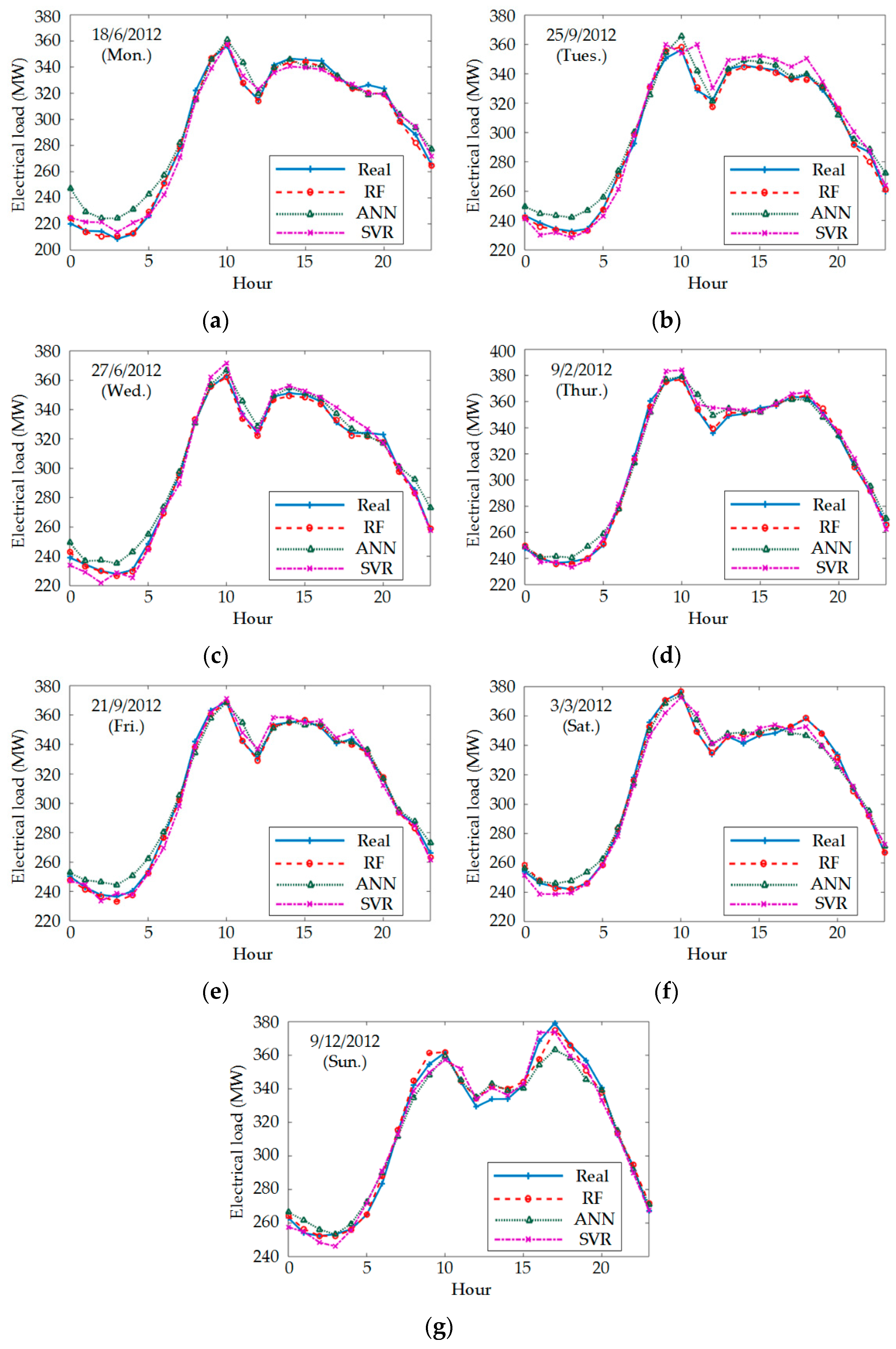
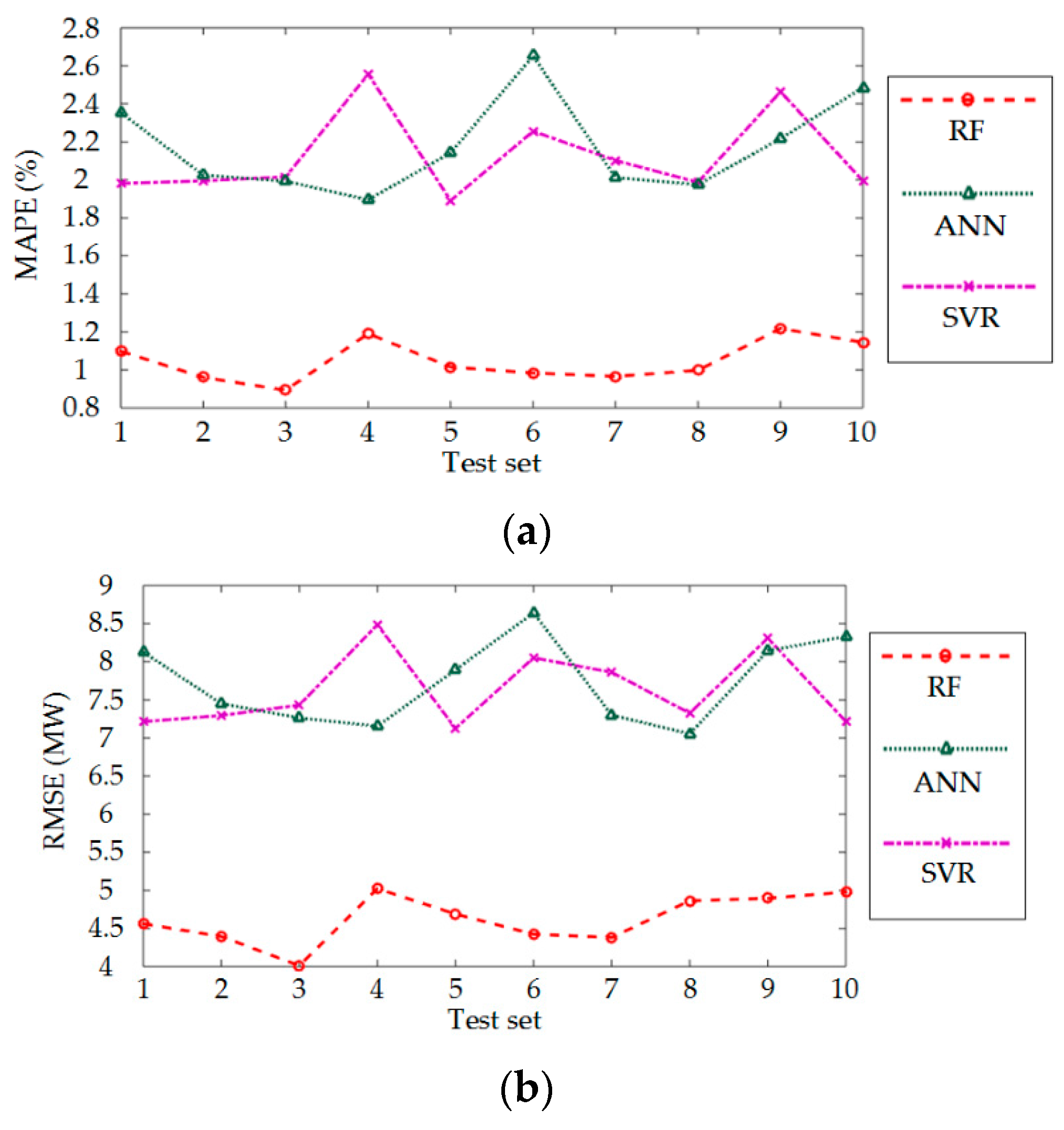
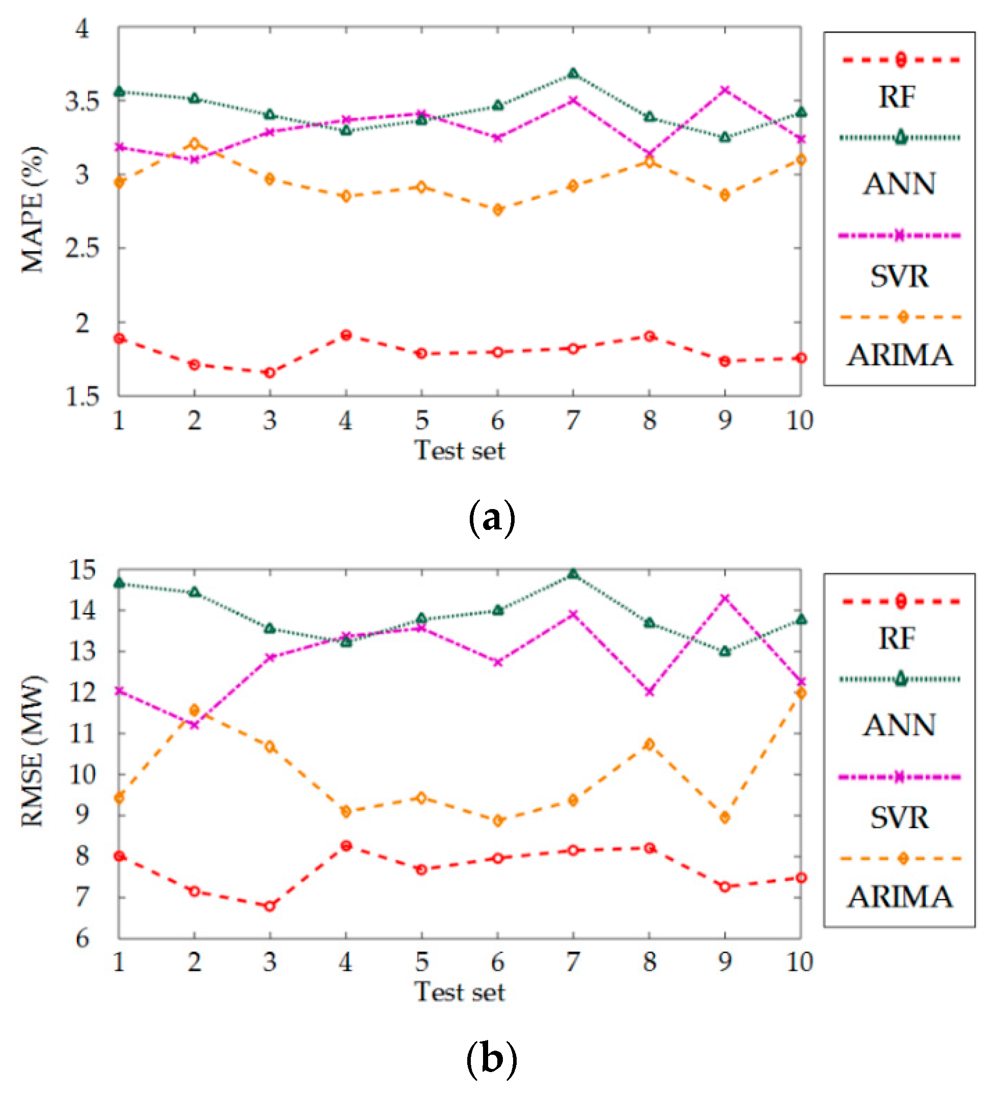
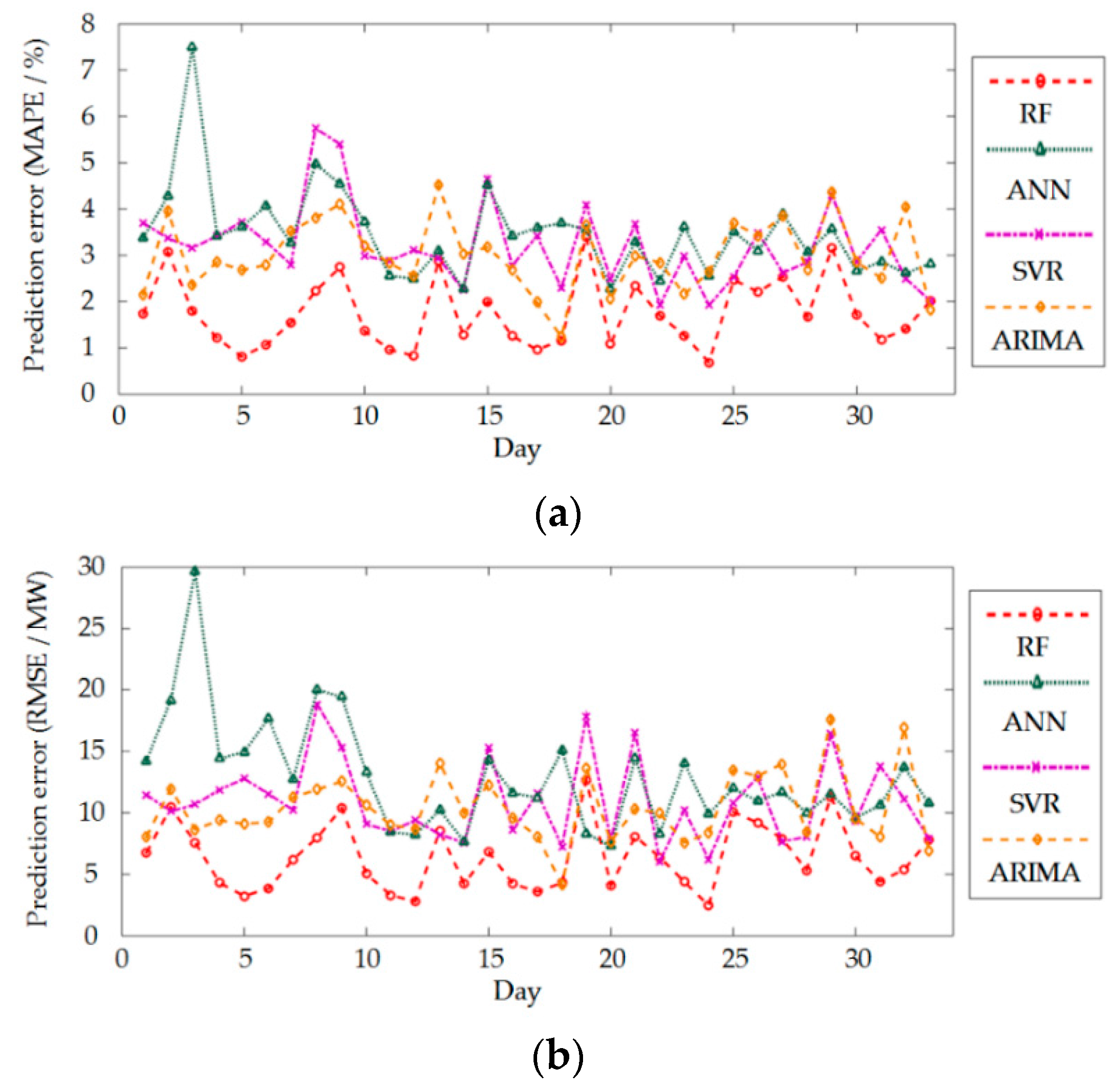
4.3. Load Forecasting Error of Different Models

The selection of predictor also significantly affects the forecasting results. Two other kinds of load predictors, namely SVR and ANN, are therefore considered to verify the effectiveness of the proposed approach for STLF.

In the comparison experiment, SVR uses the RBF Kernel function. The three major parameters, C (trade-off parameter), $\delta$ (RBF width), and $\epsilon$ (constant value), are set to 1500, 0.45, and 0.1 according to Kavousi et al. [16]. A BP neural network (BPNN) with three layers is used as the ANN model. The number of neurons in the hidden layer is determined to be 30 through experiments. The connection coefficient $w_{ij}$ between the input layer and hidden layer neurons and the connection coefficient $w_{jk}$ between the hidden layer and output layer neurons in BPNN are calculated according to reference [13].

The optimal feature subset is used as the input of RF. When SVR and ANN are used as predictors, the proposed feature selection method is repeated using SVR and ANN instead of RF. A total of 27 and 22 features are selected for SVR and ANN for 1-h-ahead prediction, and 38 and 36 features for day-ahead prediction. When the day-ahead prediction is conducted, a time series analysis method called ARIMA that lacks a feature selection process is used for comparison. The load data for 20 days before the forecast date are used as the input of ARIMA. After the training process is completed, the prediction errors on the test set are recorded. The 1-h-ahead prediction and day-ahead prediction errors of the three predictors on the test sets of different quarters and the entire test set are listed in

Table 10. Mean absolute percentage error (MAPE) and root mean square error (RMSE) of random forest (RF), support vector regression (SVR), and artificial neural network (ANN) on the different testing sets of 1-h-ahead prediction.

Time Period of Testing Set	Predict Error	Predictors/Dimension of Feature Subset
		RF/24	SVR/27	ANN/22
The first quarter	MAPE (%)	0.849	2.240	1.665
	RMSE (MW)	3.924	7.396	6.723
The second quarter	MAPE (%)	0.868	1.664	2.504
	RMSE (MW)	3.281	6.741	8.467
The third quarter	MAPE (%)	0.919	1.889	2.142
	RMSE (MW)	3.985	7.381	7.315
The fourth quarter	MAPE (%)	1.216	2.306	2.339
	RMSE (MW)	5.901	8.894	9.057
Total	MAPE (%)	0.971	2.021	2.165
	RMSE (MW)	4.372	7.448	7.926

and

Table 11. MAPE and RMSE of RF, SVR, ANN, and ARIMA on the different testing sets of day-ahead prediction.

Time Period of Testing Set	Predict Error	Predictors/Dimension of Feature Subset
		RF/33	SVR/38	ANN/36	ARIMA/480
The first quarter	MAPE (%)	1.794	3.585	4.309	2.961
	RMSE (MW)	7.659	12.884	18.546	9.586
The second quarter	MAPE (%)	1.663	3.616	3.326	3.059
	RMSE (MW)	6.187	12.652	12.211	9.833
The third quarter	MAPE (%)	1.673	3.233	3.057	2.482
	RMSE (MW)	7.057	12.279	11.506	8.179
The fourth quarter	MAPE (%)	1.987	3.058	3.074	3.145
	RMSE (MW)	7.874	11.754	11.971	9.996
Total	MAPE (%)	1.745	3.273	3.430	2.957
	RMSE (MW)	7.324	12.451	13.798	9.513

, respectively.

Table 10 indicates that, no matter which test set is used, the MAPE and RMSE generated by RF are basically only half or less of those by SVR and ANN. When the entire test set is used to test the performance of RF, the MAPE is only 0.971%. Although the MAPE and RMSE in Table 11 are larger than those in Table 10, the same conclusion can be drawn from Table 11. Therefore, RF is proven to be more suitable than SVR, ANN, and ARIMA for STLF. The real load curve and forecasting load curves of seven days of the test set obtained from 1-h-aheah prediction and day-ahead prediction are shown in Figure 7 and Figure 8, respectively. These seven days contain every day of the week and are randomly and equally extracted from four quarters (approximately two days per quarter). These seven days include June 18 (Mon.), September 25 (Tues.), June 27 (Wed.), February 9 (Thur.), September 21 (Fri.), March 3 (Sat.), and December 9 (Sun.).

Figure 7 shows that the load curve predicted by RF nearly overlaps with the real load curve. Compared with the load curve predicted by RF, the load curves predicted by SVR and ANN have a certain error with the real load curve. Although the fitting degree among all the forecasting load curves and the real load curve in Figure 8 are worse than those in Figure 7, the load curve predicted by RF is still better than the load curves predicted by SVR, ANN, and ARIMA. This result validates the high accuracy of RF when used as the load predictor. The MAPE and RMSE of different predictors of the seven days in Figure 7 and Figure 8 are shown in

Table 12. Prediction error of different predictors of the selected seven test days when 1-h-ahead prediction is conducted.

Data	Prediction Error	Predictors
		RF	SVR	ANN
June 18 (Mon.)	MAPE (%)	0.870	2.027	3.198
	RMSE (MW)	3.137	6.047	10.467
September 25 (Tues.)	MAPE (%)	0.723	2.140	1.969
	RMSE (MW)	2.813	8.879	6.711
June 27 (Wed.)	MAPE (%)	0.633	1.414	1.791
	RMSE (MW)	2.218	5.133	6.117
February 9 (Thur.)	MAPE (%)	0.557	1.282	1.436
	RMSE (MW)	2.049	5.618	5.614
September 21 (Fri.)	MAPE (%)	0.554	1.132	1.524
	RMSE (MW)	2.035	3.964	5.486
March 3 (Sat.)	MAPE (%)	0.479	1.479	1.460
	RMSE (MW)	2.103	5.638	5.351
December 9 (Sun.).	MAPE (%)	0.910	1.346	1.716
	RMSE (MW)	4.091	4.889	6.831

and

Table 13. Prediction error of different predictors of the selected seven test days when day-ahead prediction is conducted.

Data	Prediction Error	Predictors
		RF	SVR	ANN	ARIMA
June 18 (Mon.)	MAPE (%)	2.001	4.674	4.519	3.174
	RMSE (MW)	6.817	15.332	14.235	12.279
September 25 (Tues.)	MAPE (%)	0.688	1.929	2.552	2.638
	RMSE (MW)	2.448	6.208	9.923	8.352
June 27 (Wed.)	MAPE (%)	1.253	2.771	3.407	2.676
	RMSE (MW)	4.224	8.594	11.591	9.570
February 9 (Thur.)	MAPE (%)	1.215	3.423	3.419	2.854
	RMSE (MW)	4.302	11.836	14.416	9.388
September 21 (Fri.)	MAPE (%)	1.266	2.981	3.616	2.152
	RMSE (MW)	4.399	10.195	14.055	7.587
March 3 (Sat.)	MAPE (%)	1.066	3.285	4.072	2.792
	RMSE (MW)	3.839	11.537	17.692	10.491
December 9 (Sun.).	MAPE (%)	1.405	2.492	2.611	4.036
	RMSE (MW)	5.399	10.053	13.683	16.960

, respectively, when 1-h-ahead prediction and day-ahead prediction are conducted.

Table 12 and Table 13 indicate that the MAPE and RMSE of RF are always lower than those of the other methods. This result is attributed to that RF requires few parameters to be optimized and is resistant to overfitting. As a result, RF can obtain higher prediction accuracy than SVR, ANN, and ARIMA when used for STLF.

Each day of the test set is arranged according to the order of the date. The MAPE and RMSE of each test day of the three predictors for the 1-h-ahead prediction are shown in Figure 9a,b. The MAPE and RMSE of each test day of the four predictors for the day-ahead prediction are shown in Figure 10a,b.

As shown in Figure 9, when the 1-h-ahead prediction is conducted, the MAPE and RMSE produced by RF are smaller than those produced by SVR and ANN. Figure 9a shows that the MAPE of RF is higher than 1.5% only when used to forecast the load of the 26th test day, whereas the MAPE of SVR and ANN are mostly higher than 1.5%. A similar conclusion is obtained from Figure 9b. When RF is used to forecast the load, in addition to the RMSE of the 26th test day being higher than 6 MW, the RMSE of the 25th test day is slightly higher than 6 MW. As shown in Figure 10a,b, the MAPE and RMSE of RF are basically smaller than those of the three other predictors. Therefore, the accuracy of RF applied to the load forecasting was verified.

4.4. Further Validation of Effectiveness of the Proposed Method Based on 10-Fold Cross-Validation

A 10-fold cross-validation was used to fully verify the effectiveness of the proposed method. The entire dataset was randomly divided into 10 groups (six groups of 37 days and four groups of 36 days). A 10-fold cross-validation was used to analyze the prediction error of the proposed method under different test sets, in which the optimal parameters of the predictors are unchanged. The MAPE and RMSE of different predictors on the test set of 10 independent experiments are shown in Figure 11 and Figure 12 for 1-h-ahead prediction and day-ahead prediction.

Figure 11 and Figure 12 show that the MAPE and RMSE in 10-fold cross-validation experiments are consistent with the results in Table 10 and Table 11. The prediction error of RF is lower than the errors of other methods. When 1-h-ahead prediction is conducted, the MAPE of the proposed method ranges from 0.893% to 1.218%, and the RMSE ranges from 4.012 MW to 5.023 MW. It can be seen that the MAPE and RMSE of the proposed method in 10-fold cross-validation are around 0.971% and 4.372 MW, respectively, for minor fluctuation. When day-ahead prediction is conducted, the MAPE of the proposed method ranges from 1.659% to 1.912%, and the RMSE ranges from 6.795 MW to 8.268 MW. Similarly, the MAPE and RMSE of the proposed method in 10-fold cross-validation are around 1.745% and 7.324 MW, respectively, for minor fluctuation. According to the experimental results of 10-fold cross-validation, it can be concluded that the proposed method can achieve satisfactory forecast results for different training and test sets. The effectiveness and robustness of the proposed method were verified.

Therefore, RF can obtain satisfying prediction results for different test sets, and the validity and accuracy of RF applied to STLF were once again verified.

5. Conclusions

A novel feature selection method for STLF is proposed in this paper. Compared with current STLF methods and feature selection methods, the following innovations are made in this study:

• Compared with other STLF methods that use another feature selection method with high time complexity, the proposed approach designs a novel feature selection method based on PI value obtained in the training process of RF. The optimal forecasting feature subset is selected only by the improved SBS method with simple principle and high efficiency.
• In the process of feature selection, the prediction error of RF is used to determine the performance of each feature subset. Only two parameters of RF need to be adjusted, and the parameter selection method is clear. Considering this advantage, the proposed approach avoids the influence of unreasonable model parameters on the feature selection results.
• The traditional SBS method is optimized to reduce the number of iterations. Therefore, the efficiency of the search strategy is dramatically improved.

The experimental results based on real load data verify the effectiveness of the proposed RF-based feature selection method for STLF. In addition, the optimized RF has better generalization capability than SVR and ANN. Therefore, RF is suitable for STLF of power systems. Future work will focus on load forecasting in the distribution system, especially for residential load forecasting.

References

1. Khan, A.R.; Mahmood, A.; Safdar, A.; Khan, Z.A.; Khan, N.A. Load forecasting, dynamic pricing and DSM in smart grid: A review. Renew. Sustain. Energy Rev. 2016, 54, 1311–1322. [Google Scholar] [CrossRef]
2. Alvarez, F.; Troncoso, A.; Riquelme, J.C.; Ruiz, J.S. Energy time series forecasting based on pattern sequence similarity. IEEE Trans. Knowl. Data Eng. 2011, 23, 1230–1243. [Google Scholar] [CrossRef]
3. Amjady, N. Short-term bus load forecasting of power systems by a new hybrid method. IEEE Trans. Power Syst. 2007, 22, 333–341. [Google Scholar] [CrossRef]
4. Kulkarni, S.; Simon, S.P.; Sundareswaran, K. A spiking neural network (SNN) forecast engine for short-term electrical load forecasting. Appl. Soft Comput. 2013, 13, 3628–3635. [Google Scholar] [CrossRef]
5. Al-Hamadi, H.M.; Soliman, S.A. Short-term electric load forecasting based on Kalman filtering algorithm with moving window weather and load model. Electr. Power Syst. Res. 2004, 68, 47–59. [Google Scholar] [CrossRef]
6. Christiaanse, W.R. Short-term load forecasting using general exponential smoothing. IEEE Trans. Power Appar. Syst. 1971, 90, 900–911. [Google Scholar] [CrossRef]
7. Wi, Y.M.; Joo, S.K.; Song, K.B. Holiday load forecasting using fuzzy polynomial regression with weather feature selection and adjustment. IEEE Trans. Power Syst. 2012, 27, 596–603. [Google Scholar] [CrossRef]
8. Wang, J.; Wang, J.; Li, Y.; Zhu, S.; Zhao, J. Techniques of applying wavelet de-noising into a combined model for short-term load forecasting. Int. J. Electr. Power Energy Syst. 2014, 62, 816–824. [Google Scholar] [CrossRef]
9. Wang, B.; Tai, N.L.; Zhai, H.Q.; Ye, J.; Zhu, J.D.; Qi, L.B. A new ARMAX model based on evolutionary algorithm and particle swarm optimization for short-term load forecasting. Electr. Power Syst. Res. 2008, 78, 1679–1685. [Google Scholar] [CrossRef]
10. Nie, H.; Liu, G.; Liu, X.; Wang, Y. Hybrid of ARIMA and SVMs for short-term load forecasting. Energy Procedia 2012, 16, 1455–1460. [Google Scholar] [CrossRef]
11. Hinojosa, V.H.; Hoese, A. Short-term load forecasting using fuzzy inductive reasoning and evolutionary algorithms. IEEE Trans. Power Syst. 2010, 25, 565–574. [Google Scholar] [CrossRef]
12. Mamlook, R.; Badran, O.; Abdulhadi, E. A fuzzy inference model for short-term load forecasting. Energy Policy 2009, 37, 1239–1248. [Google Scholar] [CrossRef]
13. Feng, Y.; Xu, X. A short-term load forecasting model of natural gas based on optimized genetic algorithm and improved BP neural network. Appl. Energy 2014, 134, 102–113. [Google Scholar]
14. Hernández, L.; Baladrón, C.; Aguiar, J.M.; Carro, B.; Sánchez-Esguevillas, A.; Lloret, J. Artificial neural networks for short-term load forecasting in microgrids environment. Energy 2014, 75, 252–264. [Google Scholar] [CrossRef]
15. Hernández, L.; Baladrón, C.; Aguiar, J.M.; Calavia, L.; Carro, B.; Sánchez-Esguevillas, A.; Pérez, F.; Fernández, Á.; Lloret, J. Artificial neural network for short-term load forecasting in distribution systems. Energies 2014, 7, 1576–1598. [Google Scholar] [CrossRef]
16. Kavousi-Fard, A.; Samet, H.; Marzbani, F. A new hybrid modified firefly algorithm and support vector regression model for accurate short term load forecasting. Expert Syst. Appl. 2014, 41, 6047–6056. [Google Scholar] [CrossRef]
17. Che, J.X.; Wang, J.Z. Short-term load forecasting using a kernel-based support vector regression combination model. Appl. Energy 2014, 132, 602–609. [Google Scholar] [CrossRef]
18. Ceperic, E.; Ceperic, V.; Baric, A. A strategy for short-term load forecasting by support vector regression machines. IEEE Trans. Power Syst. 2013, 28, 4356–4364. [Google Scholar] [CrossRef]
19. Lahouar, A.; Slama, J.B.H. Day-ahead load forecast using random forest and expert input selection. Energy Convers. Manag. 2015, 103, 1040–1051. [Google Scholar] [CrossRef]
20. Jurado, S.; Nebot, À.; Mugica, F.; Avellana, N. Hybrid methodologies for electricity load forecasting: entropy-based feature selection with machine learning and soft computing techniques. Energy 2015, 86, 276–291. [Google Scholar] [CrossRef] [Green Version]
21. Dudek, G. Short-Term Load Forecasting Using Random Forests. Intell. Systems'2014 2015, 323, 821–828. [Google Scholar]
22. Wang, J.; Li, L.; Niu, D.; Tan, Z. An annual load forecasting model based on support vector regression with differential evolution algorithm. Appl. Energy 2012, 94, 65–70. [Google Scholar] [CrossRef]
23. Breiman, L. Random forest. Mach. Learn. 2001, 45, 5–32. [Google Scholar] [CrossRef]
24. Che, J.X.; Wang, J.Z.; Tang, Y.J. Optimal training subset in a support vector regression electric load forecasting model. Appl. Soft Comput. 2012, 12, 1523–1531. [Google Scholar] [CrossRef]
25. Ghofrani, M.; Ghayekhloo, M.; Arabali, A.; Ghayekhloo, A. A hybrid short-term load forecasting with a new input selection framework. Energy 2015, 81, 777–786. [Google Scholar] [CrossRef]
26. Kouhi, S.; Keynia, F. A new cascade NN based method to short-term load forecast in deregulated electricity market. Energy Convers. Manag. 2013, 71, 76–83. [Google Scholar] [CrossRef]
27. Breiman, L.; Friedman, J.H.; Olshen, R.A.; Stone, C.J. Classification and Regression Trees; Chapman Hall: New York, NY, USA, 1984. [Google Scholar]
28. Troncoso, A.; Salcedo-Sanz, S.; Casanova-Mateo, C.; Riquelme, J.C.; Prieto, L. Local models-based regression trees for very short-term wind speed prediction. Renew. Energy 2015, 81, 589–598. [Google Scholar] [CrossRef]
29. Sirlantzis, K.; Hoque, S.; Fairhurst, M.C. Diversity in multiple classifier ensembles based on binary feature quantisation with application to face recognition. Appl. Soft Comput. 2008, 8, 437–445. [Google Scholar] [CrossRef]
30. Li, S.; Wang, P.; Goel, L. Short-term load forecasting by wavelet transform and evolutionary extreme learning machine. Electr. Power Syst. Res. 2015, 122, 96–103. [Google Scholar] [CrossRef]
Figure 1. Flowchart of the algorithm.
Energies 09 00767 g001
Figure 2. Load curve of the entire year.
Energies 09 00767 g002
Figure 3. (a) Boxplot of the PI value of the first 122 features of 1-h-ahead prediction; (b) boxplot of the PI value of the remaining 121 features of 1-h-ahead prediction.
Energies 09 00767 g003aEnergies 09 00767 g003b
Figure 4. (a) Boxplot of the PI value of the first 122 features of day-ahead prediction; (b) boxplot of the PI value of the remaining 121 features of day-ahead prediction.
Energies 09 00767 g004
Figure 5. (a) The permutation importance (PI) values of the first 40 features of 1-h-ahead prediction; (b) The permutation importance (PI) values of the first 40 features of day-ahead prediction.
Energies 09 00767 g005
Figure 6. (a) Prediction error (MAPE) of different feature subsets obtained from SBS method of 1-h-ahead prediction; (b) prediction error (MAPE) of different feature subsets obtained from SBS method of day-ahead prediction.
Energies 09 00767 g006
Figure 7. (a) The comparison of prediction results obtained from 1-h-ahead prediction of June 18th; (b) the comparison of prediction results obtained from 1-h-ahead prediction of September 25th; (c) the comparison of prediction results obtained from 1-h-ahead prediction of June 27th; (d) the comparison of prediction results obtained from 1-h-ahead prediction of February 9th; (e) the comparison of prediction results obtained from 1-h-ahead prediction of September 21st; (f) the comparison of prediction results obtained from 1-h-ahead prediction of March 3rd; (g) the comparison of prediction results obtained from 1-h-ahead prediction of December 9th.
Energies 09 00767 g007
Figure 8. (a) The comparison of prediction results obtained from day-ahead prediction of June 18th; (b) the comparison of prediction results obtained from day-ahead prediction of September 25th; (c) the comparison of prediction results obtained from day-ahead prediction of June 27th; (d) the comparison of prediction results obtained from day-ahead prediction of February 9th; (e) the comparison of prediction results obtained from day-ahead prediction of September 21st; (f) the comparison of prediction results obtained from day-ahead prediction of March 3rd; (g) the comparison of prediction results obtained from day-ahead prediction of December 9th.
Energies 09 00767 g008
Figure 9. (a) MAPE of three predictors for each test day when 1-h-ahead prediction is conducted; (b) RMSE of three predictors for each test day when 1-h-ahead prediction is conducted.
Energies 09 00767 g009
Figure 10. (a) MAPE of four predictors for each test day when day-ahead prediction is conducted; (b) RMSE of four predictors for each test day when day-ahead prediction is conducted.
Energies 09 00767 g010
Figure 11. (a) MAPE of three predictors on the 10 test sets when 1-h-ahead prediction is conducted; (b) RMSE of three predictors on the 10 test sets when 1-h-ahead prediction is conducted.
Energies 09 00767 g011
Figure 12. (a) MAPE of four predictors on the 10 test sets when day-ahead prediction is conducted; (b) RMSE of four predictors on the 10 test sets when day-ahead prediction is conducted.
Energies 09 00767 g012