Article

A Hybrid Method Based on Singular Spectrum Analysis, Firefly Algorithm, and BP Neural Network for Short-Term Wind Speed Forecasting

1
School of Statistics, Dongbei University of Finance and Economics, Dalian 116025, China
2
Key Laboratory of Arid Climatic Change and Reducing Disaster of Gansu Province, College of Atmospheric Sciences, Lanzhou University, Lanzhou 730000, China
*
Author to whom correspondence should be addressed.
Energies 2016, 9(10), 757; https://doi.org/10.3390/en9100757
Submission received: 12 July 2016 / Revised: 14 August 2016 / Accepted: 18 August 2016 / Published: 22 September 2016
(This article belongs to the Special Issue Energy Time Series Forecasting)

Abstract

:
With increasing importance being attached to big data mining, analysis, and forecasting in the field of wind energy, how to select an optimization model to improve the forecasting accuracy of the wind speed time series is not only an extremely challenging problem, but also a problem of concern for economic forecasting. The artificial intelligence model is widely used in forecasting and data processing, but the individual back-propagation artificial neural network cannot always satisfy the time series forecasting needs. Thus, a hybrid forecasting approach has been proposed in this study, which consists of data preprocessing, parameter optimization and a neural network for advancing the accuracy of short-term wind speed forecasting. According to the case study, in which the data are collected from Peng Lai, a city located in China, the simulation results indicate that the hybrid forecasting method yields better predictions compared to the individual BP, which indicates that the hybrid method exhibits stronger forecasting ability.

Graphical Abstract

1. Introduction

Wind energy has been a fast growing energy resource type because it is renewable, pollution free and abundant. Currently, with the development of the economy, many countries are facing a severe energy crisis. Therefore, there is no doubt that the necessity of exploring and using various sources of energy will need to be emphasized. Wind energy, as one of the major renewable energy sources, is a great challenge regarding the reliability and accuracy of power systems, considering the fluctuation of the wind speed. Therefore prediction has become a theme in the planning of today’s competitive environment. Wind speed prediction is more necessary for us to explore and take good advantage of the advantages of wind power [1]. Utilizing appropriate wind speed data, power system operators are able to predict the theoretical power output, which helps in system planning, scheduling and storage capacity optimization. Thus, wind speed prediction plays an important role in actual decisions. In order to increase the accuracy of wind speed prediction, a hybrid predicted model is proposed in this paper.
A number of time series forecasting methods have been successfully applied to the short-term prediction of wind speed and power generation. The autoregressive integrated moving average (ARIMA), as a widely used approach for time series forecasting, has been employed in wind speed forecasting [2,3]. In addition, correlating with the ARIMA, a group has been set up for forecasting. This system included the moving average model (MA), autoregressive (AR), and the autoregressive moving average (ARMA). Based on the ARIMA, several modified models have been proposed, such as the factional ARIMA (FARIMA) and the seasonal ARIMA (SARIMA). However, ARIMA models have an apparent imperfections. They can only explicitly reveal the relationship between the inputs and outputs, but they are generally limited to linear forms. Therefore, machine learning (ML) and artificial intelligence (AI) approaches have also been frequently applied to wind forecasting in recent years. In the related literature, the ML/AI models reported include various artificial neural network (ANN) models, such as back propagation (BP) and radial basis function (RBF) [4,5], a support vector machine (SVM) [6], fuzzy logic [7]. On the one hand, generally, compared to the ARIMA, the machine learning and artificial intelligence models are more flexible and can perform well when studying non-linear forms. On the other hand, the relationships that the ML/AI models show are not explicit enough and, sometimes, are very computationally intensive. After being studied profoundly, these model structures are integrated with other methodologies, so new methodologies emerge, named hybrid forecasting or combined forecasting methods.
The hybrid forecasting methodology usually includes several components,which exert different functions in the hybrid models [8]. In order to predict the wind speed more accurately, this paper uses a type of hybrid forecasting method, SSA-FA-BP, to forecast the wind speed. The Back-propagation (BP) model is used as the predictor to provide the final forecast result. For a single BP model, the forecasting performance is largely affected by the sample data, so the Singular Spectrum Analysis (SSA) is employed to decompose the original short-term wind speed series into true information and the noise, which can improve the quality of the data set. Furthermore, considering the randomness of the BP, a low rate of convergence is another defect. Therefore, the Firefly Algorithm (FA) algorithm is incorporated into the hybrid model to optimize the parameters of the BP network, weakening the randomness of the network and enhancing the rate of convergence and, at the same time, preventing the BP from falling into a local optimum.
Certainly, for the basic part of this hybrid forecasting method, BP has already shown considerable performance if the network structures, learning rates, inputs, the evaluation metrics forecasting and the sites of data collection are selected appropriately, but the BP neural network can easily fall into local optima. Thus, this paper uses the FA algorithm to optimize the parameters of the BP neural network to find the optimal weights and thresholds of the whole network, which is helpful for improving the forecasting accuracy and shortening the convergence time.
The firefly algorithm is an example of swarm intelligence (SI), which belongs to an artificial intelligence (AI) discipline that became increasingly popular over the last decade [9]. Swarm intelligence is inspired by the collective behavior of social swarms of ants, termites, bees, and worms; flock of birds; and schools of fish, the individuals of which show collective behavior, for example, where to forage, when to reproduce, where to live, and how to divide the necessary tasks among the available work force [10]. FA is one of the recent swarm intelligence methods developed by Yang [11] in 2008 and is a type of stochastic, nature-inspired, meta-heuristic algorithm that can be applied for solving the hardest optimization problems. It is inspired by the flashing lights of fireflies in nature. Heuristic means “to find” or “to discover solutions by trial and error” [11]. Finally, meta-heuristic means “higher level”, where the search process used in algorithms is influenced by a certain trade-off between randomization and local search [11]. In the firefly algorithm, the ‘lower level’ concentrates on the generation of new solutions within a search space and, thus, selects the best solution for survival. On the other hand, randomization enables the search process to prevent the solution from being trapped into the local optima. The local search improves a candidate solution until improvements are detected. Note that the FA is population-based. Population-based algorithms have the following advantages when compared to single-point search algorithms [12]:
a
Building blocks are put together from different solutions through crossover.
b
Focusing a search again relies on the crossover and means that, if both parents share the same value of a variable, then the offspring will also have the same value of this variable.
c
Low-pass filtering ignores distractions within the landscape.
d
Hedging against bad luck in the initial positions or decisions it makes.
e
Parameter tuning is the algorithm’s opportunity to learn good parameter values in order to balance exploration against exploitation.
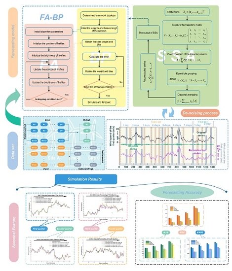
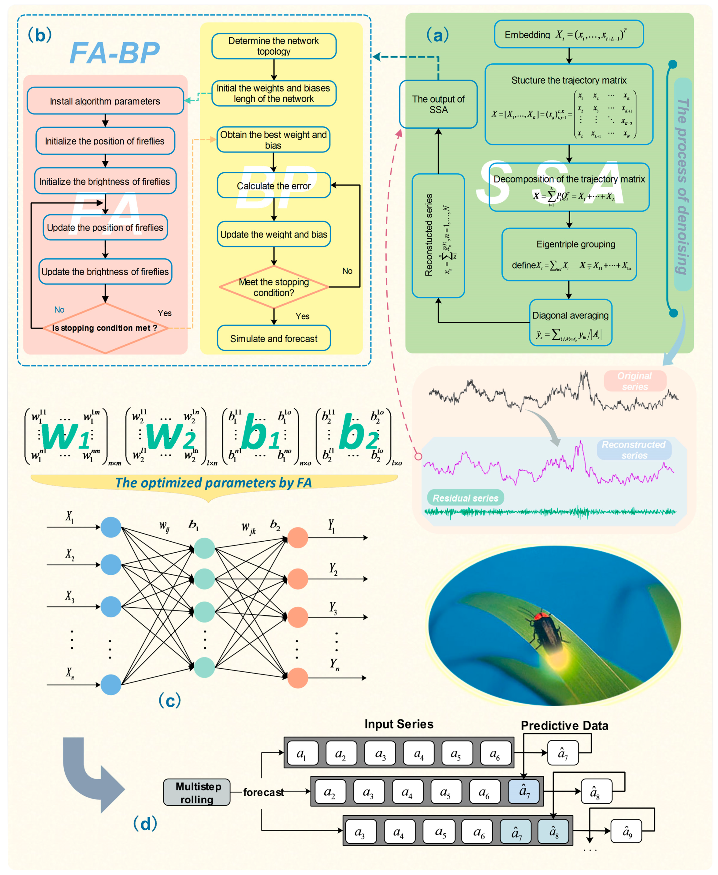
Furthermore, for most of the data of the time series, the noise components are an element that needs to be considered. Apart from the time series modeling approach, the extraction of the main features of the time series, the removal of noise and unpredictable components in a pre-processing stage can remarkably enhance the prediction performance and accuracy [13]. In fact, filtering the noisy and almost unpredictable components of nonlinear and chaotic time series by data processing techniques often leads to a series that is less complex and more predictable [14]. Here, we employed singular spectrum analysis (SSA) for de-noising. SSA works well for linear and nonlinear, stationary and non-stationary time series with different features and structure. It can efficiently identify and extract the trend and noise components of a time series [15] and then reconstruct a new series by eliminating the noise components and, hence, improve prediction performance. With this character, SSA is usually employed for time series filtering in the pre-processing stage.
The subsequent content of the paper is structured as follows: the methodologies of the individual models involved in the hybrid model are described in Section 2. Section 3 introduces the hybrid model constituted with the component models mentioned above in detail. With the hybrid models and the component models, a case study is put forward to verify the performance of the proposed models. The specific description of the data structure are explained in Section 4. Section 5 focuses on the simulation analysis, in which the results of the three experiments are displayed and analyses and comparisons of the proposed models are discussed. Finally, Section 6 presents the paper’s conclusions.

2. Methodology

In this paper, the proposed hybrid model is integrated with three components, singular spectrum analysis, the firefly algorithm, and the BP neural network.

2.1. SSA Algorithm and Methodology

In this section we introduce the information about SSA which is vital for understanding the implementation of SSA and the ways SSA has to be used for the analysis of real-life data [16]. One of basic tasks of SSA analysis is to decompose the observed time series into the sum of interpretable components with no a priori information about the time series structure. Following is the formal description of the algorithm.
Definition 1. Consider a real-value time series XN = (x1, …,xN) of length N. Let L (1<L<N) be some integer called window length and K = N − L + 1.

2.1.1. First Stage: Decomposition

The process of decomposition consist of two steps:
1st step: Embedding.
To perform the embedding we map the original time series into a sequence of lagged vectors of size L by forming K = N – L + 1 lagged vectors Xl = (x1,…,xi+L–1), i = 1…,K.
Definition 2. The trajectory matrix of the series XN is:
X = [ X 1 , X K ] = ( x i j ) i , j = 1 L , K = ( x 1 x 2 x K x 2 x 3 x K + 1 x L x L + 1 x L + 2 x N )
There are two important properties of the trajectory matrix, namely:
(a)
Both the rows and columns of X are subseries of the original series.
(b)
X has equal elements on anti-diagonals and therefore the trajectory matrix is Hankel.
2nd step: Decomposition.
Definition 3. Let { P i } i = 1 L be an orthonormal basis in RL. Consider the following decomposition of the trajectory matrix:
X = i = 1 L P i Q i T = X 1 + + X L
where Q I = X T P i , and define λ i = X i τ 2 = Q i 2 .
We consider two choices of the basis { P i } i = 1 L :
Basic: { P i } i = 1 L are eigenvectors of X X T ;
Toeplitz: { P i } i = 1 L are eigenvectors of the matrix C whose entries are:
C i = 1 N | i j | m = 1 N | i j | x m x m + | i j | , 1 i , j L
In both cases the eigenvectors are ordered so that the corresponding eigenvalues are placed in the decreasing order.
Let us remark that Case A corresponds to Singular Value Decomposition (SVD) of X, that is, X = i λ i U i V i T , P i = U i are left singular vectors of X, Q i = λ i V i , Vi are called factor vectors or right singular vectors, λi are eigenvalues of XXT; therefore, Note also that Case B is suitable only for the analysis of stationary time series with zero mean [17].
In the SSA literature (A) is also called the BK version, while (B) is called the VG one, Vi. In case A, the triple ( λ i , U i , V i ) is called the Eigen triple.

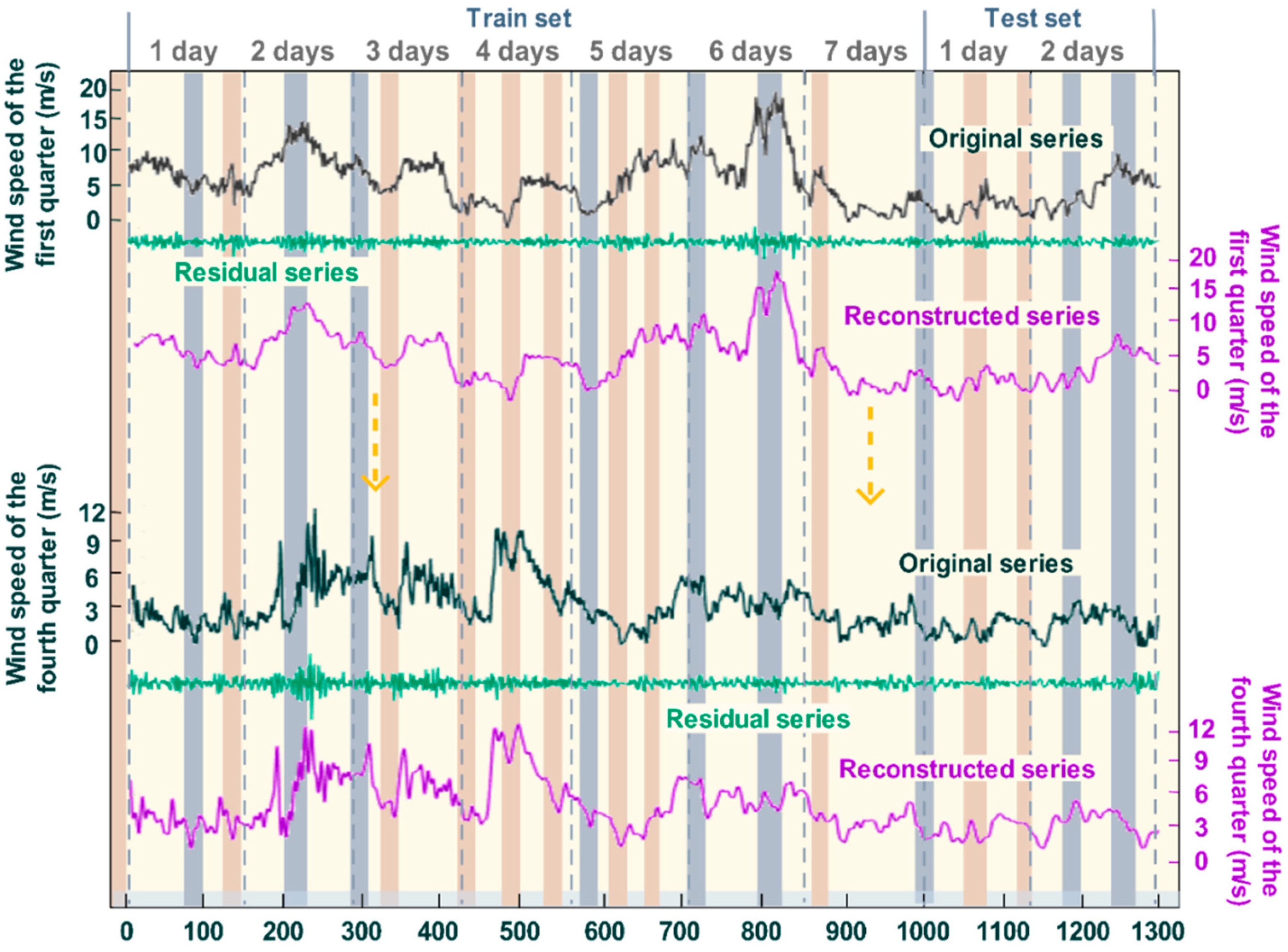
2.1.2. Second Stage: Reconstruction

The reconstruction process can be separated into two steps:
1st step: Eigen triple grouping.
Definition 1. Let d = max{j:λj ≠ 0}. Once the expansion (2) is obtained, the grouping procedure partitions the set of indices {1,…,d} into m disjoint subsets I1,…,Im. Define X I = i I X i . The expansion (2) leads to the decomposition:
X = X I 1 + + X Im
The procedure of choosing the sets I1,…,Im is called Eigen triple grouping. If m = d and Ij = {j}, j = 1,…,d; then the corresponding grouping is call elementary. The choice of several leading Eigen triples for Case A corresponds to the approximation of the time series in view of the well-known optimality property of the SVD.
2nd step: Diagonal averaging.
Definition 2. At this step, we transform each matrix Xij of the grouped decomposition (3) into a new series of length N. let Y be an L × K matrix with elements yij, 1 ≤ iL, 1 ≤ jK, and let for simplicity LK. By making the diagonal averaging we transfer the matrix Y into the series ( y ˜ 1 , , y ˜ N ) using the formula:
y ˜ s = ( j , k ) A s y j k / | A s |
where As = {(j,k): l + k = s + 1, 1 ≤ lL, 1 ≤ kK} and |As| denotes the number of elements in the set As, This corresponds to averaging the matrix element over the “antidiagonals”.
Diagonal averaging (4) applied to a resultant matrix Xjk produces a reconstructed series X ˜ ( k ) = ( x ˜ 1 ( k ) , , x ˜ N ( k ) ) . Therefore, the initial series ( x 1 , x N ) is decomposed into a sum of m reconstructed series:
x n = k = 1 m x ˜ n ( k ) , n = 1 , N
The reconstructed series produced by the elementary grouping will be called elementary reconstructed series.

2.2. Firefly Algorithm

The firefly algorithm is a popular algorithm with its basis in biology. In recent years, more and more comprehensive studies have been put forward, and its elaboration has been getting more thorough.

2.2.1. Biological Foundations

Fireflies are high-population insects, and their spectacular courtship scenes have inspired poets and scientists alike [18]. At present, there exist more than 2000 species around the world. According to several studies, the habitats of fireflies are usually warm, which implies that the swarms are more active during summer nights. Plenty of researchers have put considerable energy into the study of the firefly phenomena in nature so that many papers have been put forward, for example [19,20,21,22,23]. Fireflies are characterized by their flashing light produced by a biochemical process called bioluminescence. The flashing light serves as the primary courtship signal for mating and is also the signal for warning of potential danger. Moreover, features such as the brightness and frequency of the flashing light form the diversity of the signal. Depending on different flashing lights, the fireflies transfer information to each other and then take actions according to the message. In the FA algorithm, the brightness of the flashing light is the foremost character. Based on the brightness, the FA algorithm focuses on the movement of the fireflies when they receive brightness information, which is the biological foundation of the FA algorithm.

2.2.2. Structure of the Firefly Algorithm

FA has powerful global exploration and exploitation abilities, and it can substantially increase the local optimum avoidance ability and the convergence speed. This algorithm is based on a physical formula of the light intensity, which decreases with an increase in the square of the distance r2. However, as the distance from the light source increases, the light absorption causes that light to become weaker and weaker. These phenomena can be associated with the objective function to be optimized. As a result, the base FA can be formulated as what is illustrated in the following algorithm:
Algorithm: Pseudo-Code of the Firefly Algorithm.
1Input:
x ( 0 ) The data that has been disposed by Singular Spectrum Analysis.
x t ( 0 ) = ( x ( 0 ) ( 1 ) , x ( 0 ) ( 2 ) , , x ( 0 ) ( h ) ) - A sequence of training set.
x v ( 0 ) = ( x ( 0 ) ( h + 1 ) , x ( 0 ) ( h + 2 ) , , x ( 0 ) ( h + d ) ) —A sequence of verifying set.
2Output:
x p the value of x with the best fitness value in population of fireflies
3Parameters:
Maxgeneration—the maximum number of iterations
n—the number of fireflies
Fi—the fitness function of firefly i
xi—nest i
g—current iteration number
Li—light intensity of firefly I,
d—the number of dimension
4/*Set the parameters of FA.*/
5/* Initialize population of n fireflies xi (i = 1, 2,..., n) randomly*/
6FOR EACH i: 1 ≤ in DO
7Evaluate the corresponding fitness function Fi
8END FOR
9/*Determine light intensity.*/
10FOR EACH i: 1 ≤ in DO
11Determine light intensity Li depending on F(xi).
12END FOR
13WHILE (g < Maxgeneration) DO
14FOR EACH i = 1:n DO /*all n fireflies */
15FOR EACH j = 1:n DO /*all n fireflies */
16/*Move firefly i towards j in all d-dimensions*/
17IF (Lj > Li) THEN
18 r i j = | x i x j | = k = 1 d ( x i , k x j , k ) 2
19 x i = x i + β 0 e γ r 2 ( x j x i ) + α ( r a n d 1 2 )
20END IF
21Attractiveness varies with the distance r via β 0 e γ r 2 .
22/* Evaluate new solutions and update the light intensity. */
23END FOR j
24END FOR i
25/*Rank the fireflies and current best */
26END WHILE
/*Post process results and visualization*/
27END
There are three idealized assumptions in the FA: (1) ignorance of the sex of the fireflies, there is no difference in the firefly’s attraction between different sexes—they are considered unisexual; (2) brightness is the determining factor for the attraction of one firefly towards another which means a less bright firefly moves towards a brighter firefly. Attractiveness and brightness are in inverse proportion with the distance; (3) the landscape of the fitness function determines the brightness of a firefly.
Definition 1. The distance between any two fireflies i and j whose positions are xi and xj is given by the Cartesian distance as follows:
r i j = m = 1 D ( x i , m x j , m ) 2
where D is the number of dimensions.
Definition 2. The firefly’s attractiveness is given by:
β ( r ) = β 0 e γ r 2
At r = 0 attractiveness is β0 and γ is the light absorption coefficient. The movement of the ith firefly towards more attractive jth firefly is calculated as:
x i n e w = x i o l d + β 0 e γ r 2 ( x i o l d x j ) + α ( r a n d 1 2 )
Here, the second term represents the attraction of one firefly towards another and the randomization in the movement of firefly is caused by the third term with α as randomization parameter. Rand is random number generator. x i n e w is the new position of the ith firefly and x i o l d is the old position of ith firefly. The parameter γ determines the attractiveness and hence the speed of convergence. In implementation, we can take β0 = 1 and α ≈ (0,1). In this paper we have set γ = 0.001 however the results do not show much variation with change in value of γ.

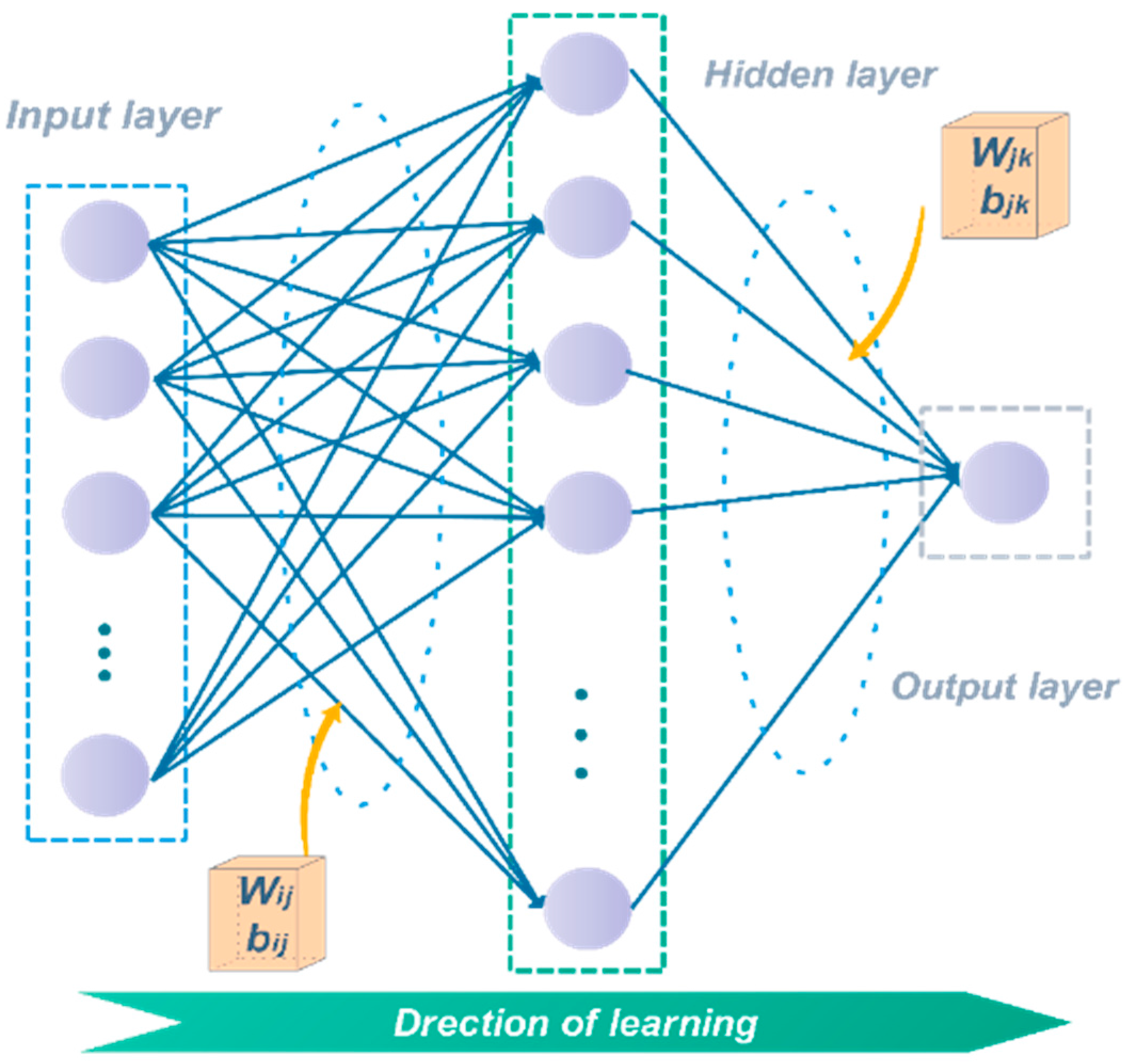
2.3. BP Neural Network

The BP neural network is a typical feed forward network. Its structure is comprised of the input layer, output layer and hidden layer, as shown in Figure 1. The working process of BP neural network can be divided into two stages: the learning stage and the working stage. In the learning stage, the input information will be disposed from input layer to the hidden layer and then to the output layer.
According to the simulation output, the differences between the results of output layer and the output given in the sample will be calculated as the back propagation of errors which will be sent back as the feedback. Depending on the feedback, the weight values (wij, wjk) and the threshold values (a, b) will be modified for the next learning cycle. By this mechanism, the connection weight of neutrons among different layers can be adjusted. When working well, the network will be applied into the working stage, in which, the input information is forward-propagating, and the output will be displayed according to the neural network [24].

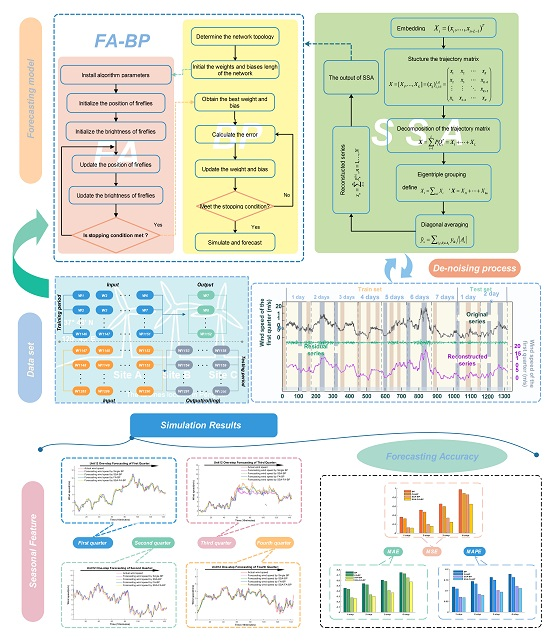
3. Hybrid SSA-FA-BP Model

The hybrid model used in this paper consists of the singular spectrum analysis, firefly algorithm, and BP neural network. Singular spectrum analysis is used to de-noise the wind speed data for preprocessing. The BP neural network is the main predicting model. The firefly algorithm is used to optimize the parameters wij, wjk, aj, and bk of the BP neural network.
The BP neural network objectively has imperfect aspects, such as susceptibility to the initial parameters of the network and easily being trapped in local optima. Therefore, the single BP neural network cannot provide good predictions because of the complexity of the short-term wind speed series. Hence, a hybrid approach consisting of SSA, FA and BP is proposed. The structure of the proposed SSA-FA-BP is shown in Figure 2.
The specific hybrid model can divided into four stages. The general task in each stage is described as follows:
Stage 1 According to the characteristics of the dataset of the BP neural network, the data have to be divided into different parts, including a training set and a test set. The training set is used to train the original network, which is built for forecasting. The test set is applied to the network to output the forecasting value.
Stage 2 Utilize singular spectrum analysis to divide the original short-term wind speed series into two modes, including a de-noising series and a residual series. Discard the residual series to de-noise and smooth the original short-term wind speed data, and make preparations for the following forecasting. In this stage, only the wind speed data of the training set are disposed by SSA. The decomposed residual series are discarded because the residual is small and can be regarded as an uncorrelated white noise series, which have a negative influence on the prediction; the rest of the decomposed modes are aggregated into the new data series. This process de-noises the original data to improve the prediction accuracy.
Stage 3 Optimize the parameters of the BP with the firefly algorithm. The FA was selected as the optimization instrument to obtain better parameters in the training process of BP, which can improve the forecasting accuracy. The FA randomly generates the initial population of the candidate solutions for the weights of the BP. After that, it calculates the light intensity of all fireflies and finds the most attractive firefly (the brightest firefly) within the population. Then, it calculates the attractiveness and distance for each firefly to move all fireflies towards the most attractive firefly in the search space. Next, the best solution among the population is passed to the BP as the initial solution.
Stage 4 Forecast the wind speed in different forecasting horizons (one-step ahead prediction or multi-step ahead prediction). After optimization of the initial parameters of the BP by the firefly algorithm, the better-trained BP is used to predict the wind speed in different forecasting horizons. The forecasting horizon in this paper is spread from one to six, which has been demonstrated to be valid.

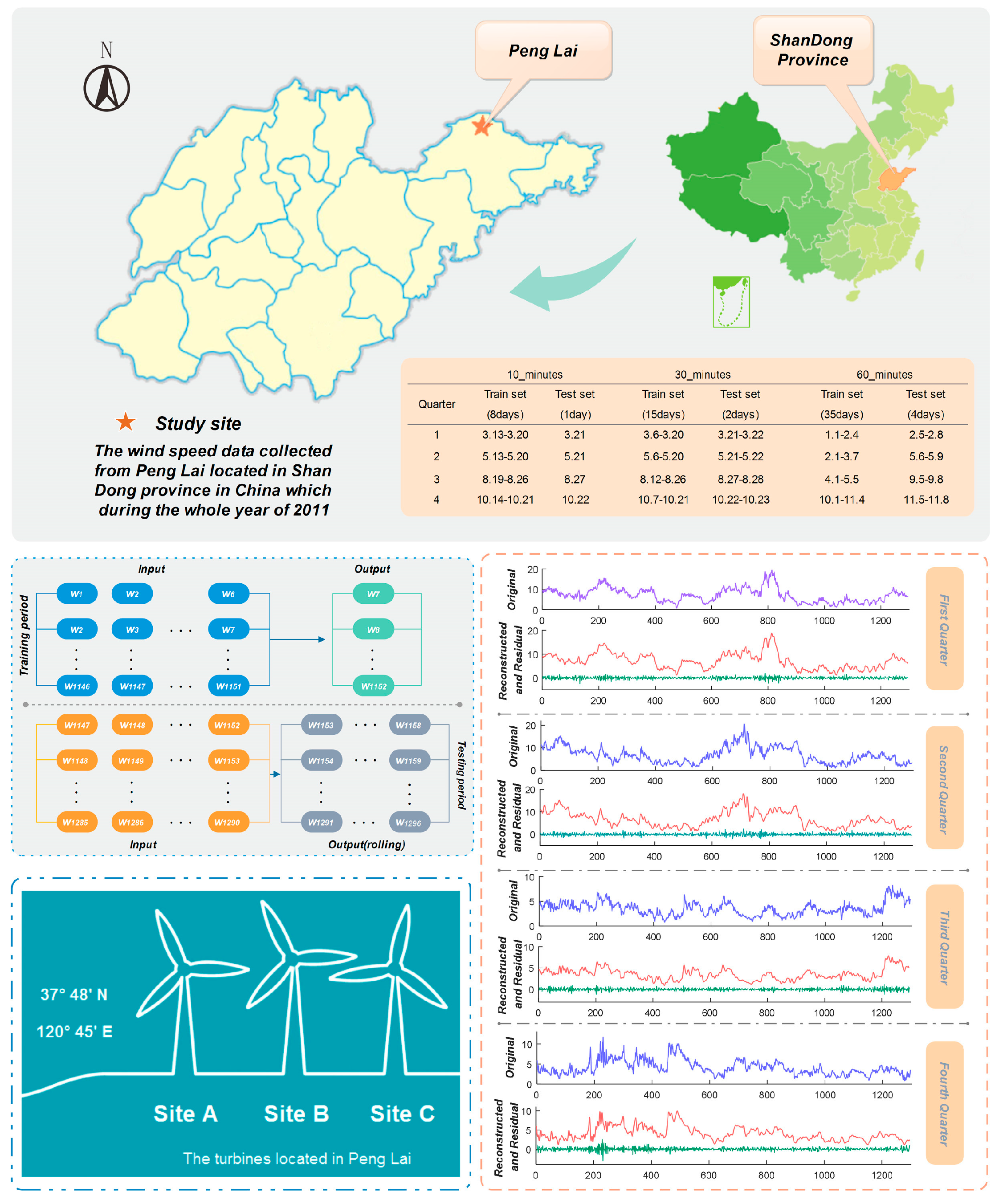
4. Brief Description of the Case Study

As a type of non-polluting and abundantly reserved energy, wind power has important significance for the sustainable development of energy. Thus, research on wind speed is necessary. In order to verify the superiority of the hybrid SSA-FA-BP model and the optimizing effect of our algorithms in actual experiments, we focus on a case study to research the forecasting function of the hybrid model in wind speed prediction.

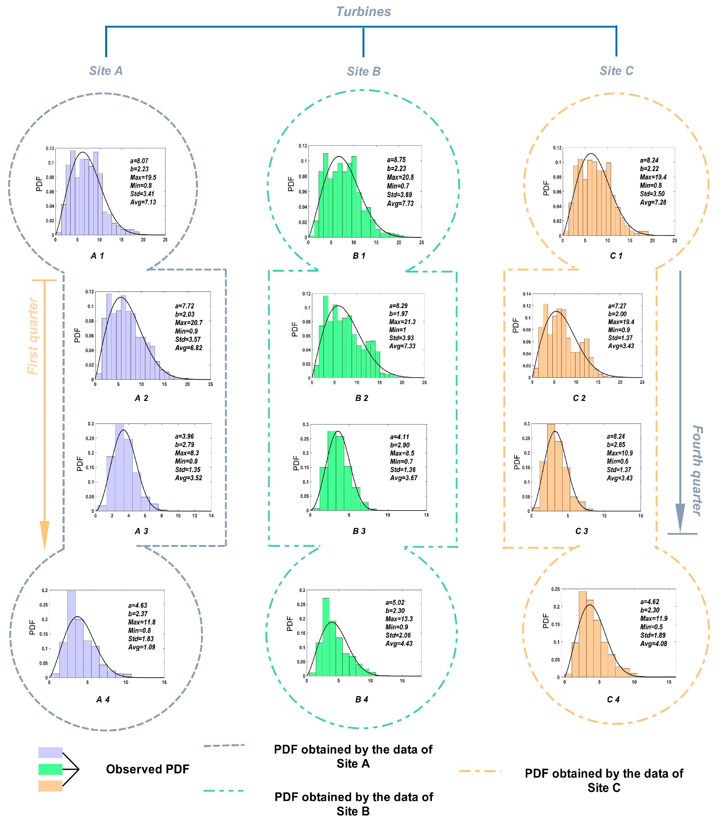
4.1. Data Collection

Considering the object that we study, wind speed data constitute the main data set of the experiment. Therefore, we choose Peng Lai as an experimental site, where wind speed data are of high quality. Peng Lai (shown in Figure 3), located in the Shandong Province in China, is a coastal city. Because of its temperate continental monsoon climate, Peng Lai has rich wind power storage capabilities. In this paper, the wind speed observations were collected from the Peng Lai wind farm to verify the proposed hybrid approach.
The data used are the wind speed data of 2011, and three main units, No. 12, No. 13, and No. 14, are selected to be studied for examining the hybrid approach. Table 1 shows the information of the different data sets. The accurate prediction of the wind speed contributes to planning the economic load dispatch and the load increment/decrement decisions made. However, according to the actual study, in order to guarantee the accuracy, the range of short-term predictions is usually considered to be 10 min to 6 h ahead [25]. The horizon is one to six steps, which definitely indicates 10 min to 6 s ahead considering all three experiments of different time intervals.
Figure 4 displays the basic statistical indexes, which include the maximum, minimum, average and standard deviation of the wind speed data involving the three experimental sites. As shown in Figure 4, the average and maximum speeds occur in Site B for four different quarters, whereas the minimum speeds occur in different seasons and sites.
The wind speed series of Site C present the maximum standard deviation values, which lead to the largest degree far away from the corresponding average value for different seasons. However, these basic statistical indexes might be not enough for surveying the wind speed patterns. In order to describe the wind speed series more adequately, the observed frequency distribution (Weibull distribution) is shown in Figure 4. According to the maximum likelihood (ML) method, the shape parameter and scale parameter in the Weill function are estimated depending on the daily wind speeds recorded in three sites [26]. For each case, the shape parameter a and the scale parameter b vary from one site to the other two sites or from one season to the other three seasons at the same site, which indicates the wind speed patterns vary significantly.

4.2. Evaluation Indices for Forecasting Performance

In this paper, in order to inspect the effect of the hybrid model, three main statistical indices are employed to measure the forecasting accuracy. They are the mean absolute percent error (MAPE), mean absolute error (MAE) and mean square error (MSE), for which small values indicate high forecast performance. These indices are defined as follows:
M A P E = 1 N n = 1 N | y n y ˜ n y n | × 100 %
M A E = 1 N n = 1 N | y n y ˜ n |
M S E = 1 N n = 1 N ( y n y ˜ n ) 2
where yn is the observed value for the time period t and y ^ n is the predicted value for the corresponding period. The MAE reveals how similar the predicted values are to the observed values, whereas the MSE measures the overall deviation between the predicted values and the observed values. The MAPE is a unit-free measure of accuracy for the predicted wind series and is sensitive to small changes in the data. According to some empirical studies, these three indices are reliable for wind speed forecasting, and have been widely used [27], but when the result of wind speed forecasting is applied to the wind power forecasting, more error would be displayed, because of other factors that have influence on the generation of wind energy, such as the turbine efficiency [28]. Therefore, the evaluation indices of wind speed forecasting are not directly applied to the management of connected electric power systems.

5. Simulation

The simulation includes three experiments, which are determined with time spans of 10, 30 and 60 min. In each experiment, three turbines (Unit 12, Unit 13, and Unit 14) are observed. For the single turbine, the observed data are divided into four quarters to facilitate the observation of the seasonal differences. The main models involved in this paper are single BP, FA-BP, SSA-BP, and SSA-FA-BP. With these four models, the forecasting data and series will be output, and in this paper, we focus on the one step and multistep prediction. The result of the 1-step, 2-step, 3-step, and 6-step predictions will be displayed in three experiments, and the main indexes for accuracy observation are MAPE, MSE, and MAE, which will be shown in all three experiments to express the superiority and inferiority of the different models.

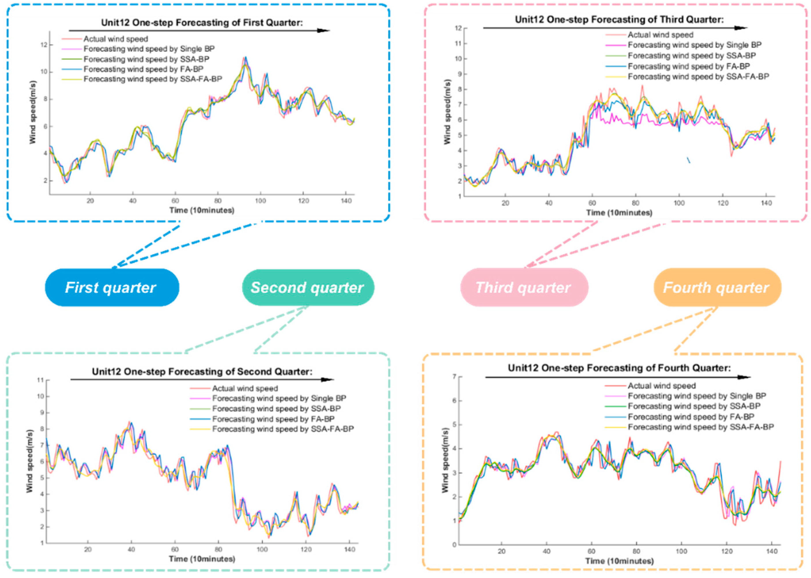
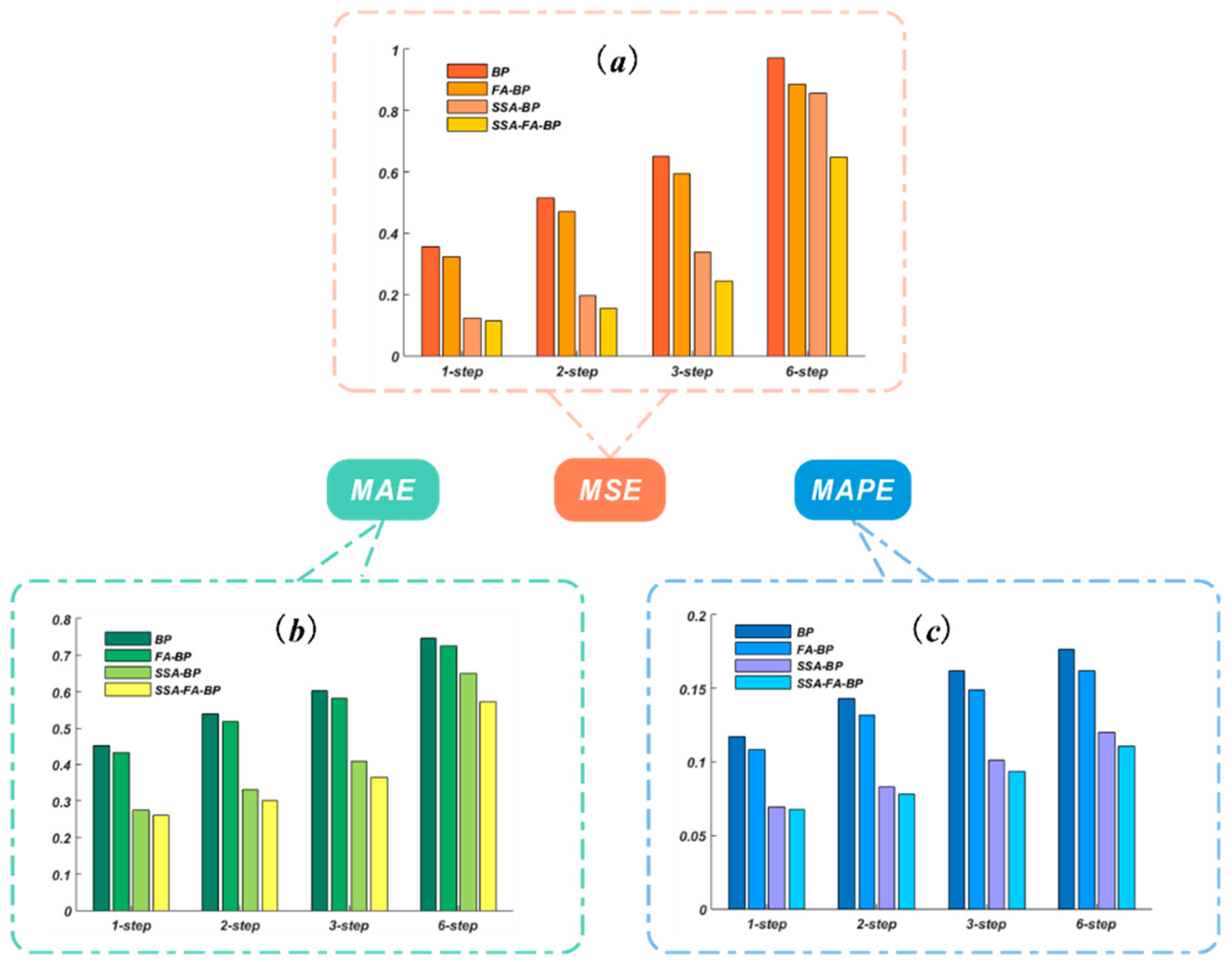
5.1. Experiment I: The Forecasting for a Time Interval of 10 Min

The experiment of 10 min takes the data of Unit 12 as an example. The original wind series presents high fluctuation and instability, as Figure 5 shows. Arranged by the SSA algorithm, the original wind speed series is decomposed, and the residual series are extracted against a meaningful series (reconstructed series). The residual series mainly contains noisy signals that will disturb the forecasting process. Therefore, before the final prediction, a de-noising process is necessary, which is able to improve the forecasting quality of the short term wind speed. During this process, the residual series are discarded, and all the other modes are reconstructed into the new series to be used for forecasting.
In this case, the number of neurons was determined by the method of trial and error. To set up a more effective network, many experiments were conducted, and then, the best trial results were selected. The experimental parameters of the BP are shown in Table 2. With many trials, for the hidden layer, when neuron number in the hidden layer was 13, the outputs showed good performance in the accuracy of forecasting. Thus, the structure of the BP was set as 6-13-1.
Table 3 shows the evaluation results for the individual forecasting and combination forecasting for the three sites (Unit 12, Unit 13, and Unit 14). It is apparent that the forecast accuracy of the proposed combination approach, SSA-FA-BP, is similar to or exceeds the single forecasting model BP and two-component models, FA-BP and SSA-BP, in all horizons for three sites. This result reflects the reliability of the proposed combined method in view of the stochastic nature of wind and its spatial and temporal variations. More detailed analyses are described as follows. Firstly, the one-step forecasting results obtained from the foresaid models will be discussed in detail. Then, we analyze the multi-step forecasting results in a similar way. Finally, we concentrate on the details of the seasonal influence to the models of concern.

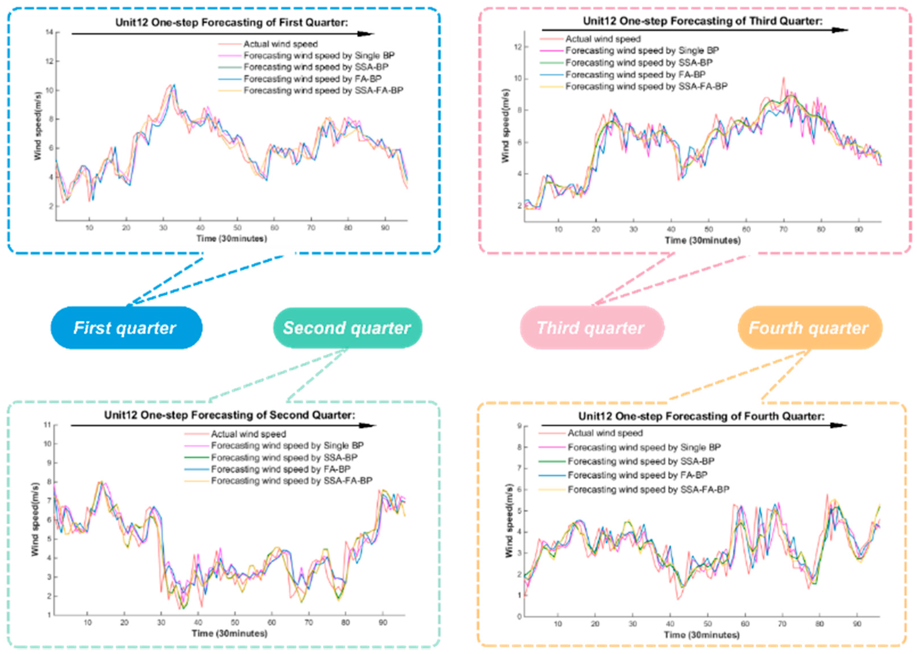
5.1.1. Analysis of One-Step Forecasting

When considering the one-step and multi-step forecasting, the accuracy indices refer to the average of the seasonal indices. For one-step forecasting, we make comparisons between the BP, FA-BP, SSA-BP and hybrid SSA-FA-BP model. The one-step ahead predicted output of the different models is displayed in Table 3. It is also clear from Table 3 and Figure 6 that the three forecasting evaluation indices (MAE, MSE and MAPE) obtained through the proposed hybrid strategy are smaller than those obtained from other component models mentioned above for all three units. Comparing the predictions shows that the integration of the SSA algorithm and the FA algorithm is an effective method for short-term wind speed prediction and that the hybrid model can provide better prediction based on the properties of the short-term wind series.
To obtain detailed properties, the models are submitted to further careful analyses. Setting Unit 12 as an example, firstly, the single BP model is used as a baseline to benchmark the forecasting accuracy, and the other combined models are compared with it. Table 3 shows that the FA-BP, SSA-BP and hybrid SSA-FA-BP models perform better than the single BP model, which reveals that the SSA and FA have good performance by improving the accuracy of forecasting. This is the reason that an increasing number of studies have proposed the de-noising algorithm and optimization algorithm to tackle short-term wind speed problems. In the comparison and analysis of forecasting, the results between the single BP and SSA-FA-BP reveal that the proposed model leads to reductions of 4.39% in MAPE, 0.14 in MAE and 0.21 in MSE. In addition, the results between the single BP and FA-BP show that the firefly algorithm leads to improvements in the accuracy of 1.3% in MAPE, 0.02 in MAE, and 0.04 in MSE. Furthermore, the results between the single BP and SSA-BP models reveal that the proposed model leads to reductions of 4.28% in MAPE, 0.14 in MAE and 0.19 in MSE. In conclusion, the model comparisons show that the proposed SSA-FA-BP hybrid model achieves better forecasting performance than the other component based on analyses of the prediction results. The SSA model has a better contribution than FA in the improvement of the forecasting accuracy. Overall, in the hybrid model, SSA-FA-BP, the SSA is more significant than the FA in improving the forecasting accuracy.

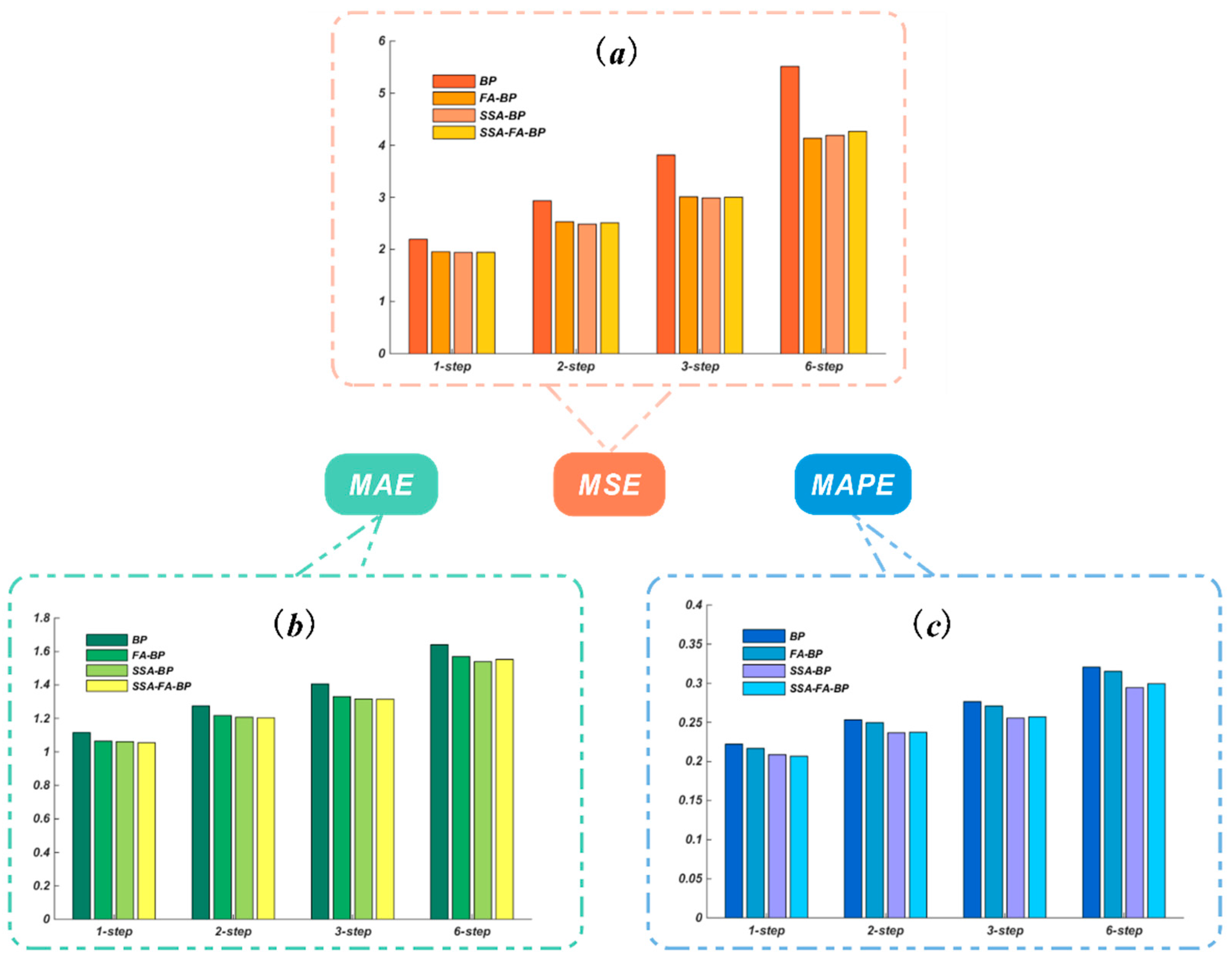
5.1.2. Analysis of Multi-Step Forecasting

The proposed hybrid SSA-FA-BP model also performs well when applied to multi-step forecasting. With the model of rolling prediction, the results of the multi-step forecasting are obtained, which involve the two steps, three steps and six steps. In the experiment of the 10 min interval, multi-step forecasting indicates forecasting for 20 min, 30 min, and one hour, as shown in Table 3 and in Figure 6.
We also find that the hybrid SSA-FA-BP exhibits better performance than the single BP model, which reveals that the models that use singular spectrum analysis and the firefly algorithm to handle the BP neural network predicted model outperform the single BP model, although the former are more complex and unintelligible than the latter. As shown in Table 3, for Unit 12, the main evaluation index MAPE of BP is 14.50% in two-step forecasting, 16.32% in three-step forecasting and 18.18% in six-step forecasting. According to relative research about wind speed forecasting, this accuracy is not sufficiently accurate for reference. However, for the hybrid model SSA-FA-BP, the corresponding index MAPE is 8.18% in two-step forecasting, 9.29% in three-step forecasting and 15.33% in six-step forecasting. Compared with the single BP, the hybrid model shows evident forecasting accuracy improvement. However, for the horizons that are more than six steps, the result of the prediction is not good enough in the condition of a time horizon of 10 min. In addition, compared with the FA-BP model, the SSA-FA-BP model leads to a 4.6% reduction in the total MAPE for the two-step prediction and a 5% reduction in the total MAPE for the three-step ahead prediction, which demonstrates that the firefly algorithm methods are effective in boosting the multi-steps forecasting accuracy of the short-term wind speed prediction. Similarly, in the comparison between the BP, SSA-BP, and SSA-FA-BP, the modified function of the SSA and FA come out. Additionally, in the hybrid model, SSA-FA-BP, the singular spectrum analysis occupied more proportions than the firefly algorithm in improving the effect of multi-steps forecasting. The hybrid models make full use of data preprocessing methods and take good advantage of the optimization algorithm to improve the performance of forecasting. In addition, with the comparison of the results of the different predicted horizons, we can draw the conclusion that the forecasting accuracy of each model decreases with an increase in the number of horizon steps.
Considering the different sites of concern, the experiment also demonstrates that the hybrid model is effective for all the data of Unit 12, Unit 13, and Unit 14, which can prove the universality of the model. According to the diversity of the experimental data, as shown in Table 3, the forecasting accuracy has a subtle distinction.

5.1.3. Analysis of Seasonal Feature

The specific seasonal forecasting results are shown in Table 4. According to the displayed accuracy indications (MAPE, MAE, and MSE), differences of accuracy caused by observation time come out. For example, in the experiment of 10 min, SSA-FA-BP model applied to the data of Unit13 in the first quarter perform the most accurate forecasting in one-step ahead, and the MAPE is 4.18%, which is a relatively ideal for wind speed forecasting. As what is shown in Figure 7, in the comparison of seasonal forecasting, for the 10-min forecasting, the forecasting accuracy of the first quarter is the best, and forecasting of the second and the fourth quarter is not good enough. Especially, for several specific sites and quarters, the SSA-FA-BP even perform worse than SSA-BP or FA-BP, which still outperform than single BP.

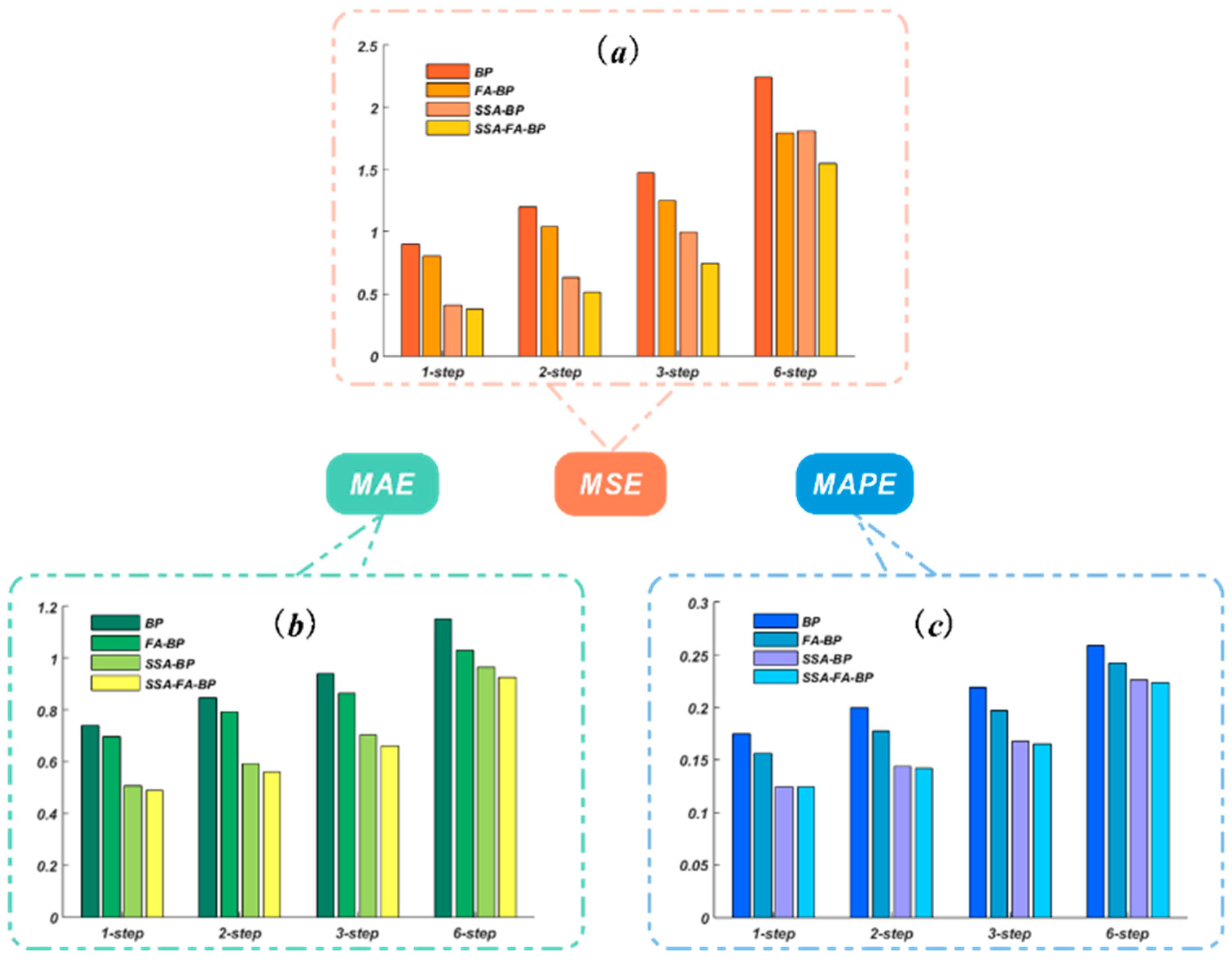
5.2. Experiment II: Forecasting for a Time Interval of 30 Min

In the 30 min experiment, the forecasting time interval is longer than the 10-min experiment. The data collected for this experiment is aimed at the whole hour point and the half hour point. The result of the forecasting is similar to the 10 min forecasting.
For example, as Table 5 shows, for Unit 12, the SSA-FA-BP model outperforms the other component models in one-step ahead forecasting and has a lower MAPE value of 12.65% compared to the MAPEs of 12.78%, 17.11% and 17.62% for the SSA-BP, FA-BP and single BP models, respectively. In Table 5 and Figure 8 the SSA-BP method performs slightly worse than the best component model in one-step ahead and multiple steps-ahead forecasting. For the FA-BP and single BP, the forecasting accuracy is obviously worse than the other two component models. As the forecasting horizon increases, the MAPEs, MAEs, and MSEs of each model increase. For Unit 13 and Unit 14, the forecasting accuracy is shown in Table 5. The wind speed forecast displays the same trend with Unit 12, which adds more weight to the universality of the effectiveness of the models. For all horizons, the SSA-FA-BP model obtains the best forecasting performance compared with other component models. The proposed approach, SSA-FA-BP, has a higher reliability and precision at all sites in terms of the forecasting performance. Table 5 shows the evaluation results of the predictions obtained from models that used SSA and FA and models that did not use SSA and FA for site 12, site 13 and site 14. The model comparisons demonstrate that the preprocessing method SSA is effective in increasing the forecasting accuracy of short-term wind speed prediction, and the optimized method FA is effective in improving the forecasting accuracy of BP. Considering the seasonal factor, the results in Table 6 and Figure 9 show that the forecasting of the wind speed in the first quarter is still the most accurate among the whole year in the 30 min experiment. However, for the second and fourth quarters, the results are not desired. For some outputs of forecasting, such as the three-step forecasting of Unit 14 in the fourth quarter, the MAPE of SSA-FA-BP is 24.81%, which is larger than SSA-BP. As the horizon increases, the number of occurrences of the abnormal results increases.

5.3. Experiment III: The Forecasting for Time Interval of 60 Min

In the experiment of 60 min, the forecasting time interval is longer than the 10 min and the 30 min experiment. The datum collected for experiment are the whole hour point. And the results of forecasting are shown in Table 7.
For example, as Table 7 shows, for Unit 12, the SSA-FA-BP model outperforms the other component models in one-step ahead forecasting and has a lower MAPE value of 20.67% compared to MAPEs of 20.88%, 21.68% and 22.22% for the SSA-BP, FA-BP and single BP models, respectively. In Table 7 and Figure 10 the SSA-BP method performs slightly worse than the best component model, in one-step ahead and multiple steps-ahead forecasting. For the FA-BP, and single BP, the forecasting accuracy is obviously worse than the other two component models. As the forecasting horizon increases, the MAPEs, MAEs, and MSEs of each model increase.
For Unit 13 and Unit 14, the forecasting accuracies are shown in Table 7. Although the optimizing effect of SSA and FA is still obvious, for the experiment of 60 min, the forecasting accuracy is generally not ideal. As Figure 10 shows, the superiority of the proposed model decreased, and the differences among the models also diminish. Considering the seasonal factor, the results in Figure 11 and Table 8 show that the forecasting of wind speed in the fourth quarter is the most accurate during the whole year in the 60 min experiment. Similarly, for the other three quarters, the results are not desirable.

5.4. Summary: Based on Experiments I–III

Comparing the three experiments above, we obtain the following overall conclusion:
The BP network has acceptable accuracy in the forecasting of the wind speed.
The combined model possesses a more powerful forecasting ability than the individual model. As every experiment shows, the accuracy of the model single BP, FA-BP, SSA-BP and SSA-FA-BP for wind speed forecasting increases successively, and in all predictions, the SSA-FA-BP almost always outperform the other two component models and the individual model.
According to the results shown in Table 3, Table 5 and Table 7, compared with BP, SSA-BP has more obvious improvement than FA-BP. Therefore, we can deduce that, in the combined model SSA-FA-BP, the SSA has more contribution than FA in the improvement of the wind speed forecasting accuracy. However, as Figure 6, Figure 8 and Figure 10 show, as the intervals of the data increase, the differences of accuracy for the models decrease, and the optimizing effects of SSA and FA decrease.
Table 9 shows the forecasting results of the three experiments with the average of the three sites. For one-step ahead forecasting, the MAPE of 10 min is 6.76%, which is less than that for 30 min and 60 min. For two-step and other multi-step ahead forecasting, the accuracy also decreases as the time interval increases.
As Table 3, Table 5, Table 7, and Table 9 show, whichever the experiment, for any model, as the forecasting horizon increases, the forecasting accuracy shows an obvious decrease. For the six-step ahead forecasting, most of the MAPE is more than 15%, which is not credible enough for wind speed forecasting. This result implies that, if the forecasting horizon is more than six, the models we propose are not available.
Figure 7, Figure 9, and Figure 11 and Table 4, Table 6, and Table 8 show that the wind speed forecasting of the first quarter is the most accurate of the whole year. The forecasting of the second and fourth quarters are not relatively ideal.

6. Statistical Testing of the Predictive Accuracy

The statistic testing has been widely used to evaluate the predictive accuracy between the various predicting models. In order to promote the superiority and conviction of the proposed model, in this paper, the bias-variance statistics framework and the Diebold-Mariano (DM) test are employed to test the predicting results at the point of statistics.

6.1. Bias-Variance Statistics Framework

The bias-variance framework [29] is utilized to estimate the models’ accuracy and stability, which are important in evaluating the effectiveness of the wind-speed forecasting models. The error attributed to bias is taken as the difference between the forecasts of the proposed model and the observed value. The error attribute to variance is taken as the variability of the forecasting results:
Definition 1: ε = x i f x i a is the difference between the forecasting value x i f and the actual value x i a . E ( x f ) = i n i = 1 n x i f is the expectation of the forecasting data, where n is the number of data for comparison. The bias-variance statistic framework is described as follows:
E ( x f x a ) = E [ x f E ( x f ) + E ( x f ) x a ] = E [ x f E ( x f ) ] 2 + [ E ( x f ) x a ] = V a r ( x f ) + B i a s 2 ( x f )
Var(xf) demonstrates the stability of predicting model, and Bias(xf) demonstrates the predictive accuracy.
Table 10 shows the bias and variance of the bias-variance statistic framework. For all three experiments of different time interval, the bias of the SSA-FA-BP is smaller than the other three models which indicate that the proposed hybrid model has is superior in predictive accuracy. However, for the same models, as the time interval increases, the bias maintains a growing trend, which reveals the decline of the accuracy. The variance results show that the proposed model is more stable generally.

6.2. The Diebold-Mariano (DM) Test

The Diebold-Mariano (DM) test [30], which is a comparative test that focuses on the predictive accuracy, could be used to compare and evaluate the forecasting performance of the proposed hybrid model and other comparing models. In empirical applications, it is often the case that two or more time series models are available for forecasting a particular variable of interest.
Definition 1. The actual values are { y n } , and the two forecasting values are { y ˜ n ( 1 ) } , and { y ˜ n ( 2 ) } . The forecasting errors from the two models are δ n ( 1 ) = y ˜ n ( 1 ) y n and δ n ( 2 ) = y ˜ n ( 2 ) y n . Here we employ the popular loss expression, absolute deviation loss, L ( δ n i ) = | δ n ( i ) | .
Definition 2. The DM test statistic evaluates the forecasts in terms of the absolute loss function:
D M = k = 1 n ( L ( δ k ( 1 ) ) L ( δ k ( 2 ) ) ) / n S 2 / n S 2
where S2 is an estimator of the variance of d k = L ( δ k ( 1 ) ) L ( δ k ( 2 ) ) .
The DM testing is based on the hypothesis testing, thus we construct the null hypothesis and the alternative hypothesis as:
H 0 : E ( d k ) = 0
H 1 : E ( d k ) 0
The null hypothesis is that the two forecasts have the same accuracy. The alternative hypothesis is that the two forecasts have different levels of accuracy under the null hypothesis, the test statistics DM is asymptotically N(0,1) distributed. The null hypothesis of no difference will be rejected if the computed DM statistic falls outside the range of [z–α/2, zα/2] that is if:
| D M | > z α / 2
where zα/2 is the upper z-value from the standard normal table corresponding to half of the desired level of the test.
The results of the DM testing are shown in Table 10. For experiment I and experiment II, the values of the DM statistic between the proposed hybrid model and the other three models are larger than the upper limit at a 1% significance level, which means the hybrid model displays a distinct superiority over the other three models. For experiment III, the value of the DM statistic between the hybrid model and BP is larger than the upper limit at 1% significance level, but for the FA-BP and the SSA-BP, the values of the DM statistic against the hybrid model are larger than the upper limit at a 10% significance level and a 15% significance level respectively, which indicates a weaker significant difference compared to the other models. Thus, it can be concluded that the hybrid model reveals a significant superiority compared to the other models for the forecasting accuracy, and as the data time intervals increase, the superiority declines.

7. Conclusions

As the energy pressure increases, the development and utilization of new renewable energy sources deserve greater attention to achieve the aims of sustainability and environmental protection. At present, there is no doubt that wind energy is one of best forms of non-renewable energy. However, for wind power generation, the reliability and accuracy of wind speed forecasts are vital, but the complexity and fluctuation of wind speed series make it a great challenge to forecast the wind speed precisely. A large number of studies have been devoted to improving wind speed forecasting performance through parameter optimization and factors analysis, which affect the final estimates significantly. However, in conventional studies, the model constructed ignoring the pre-processing of the data, which contains considerable irrelevant factors, will inaccurately estimate the fluctuation trend of the wind speed series, which is usually devoted to the deviation and errors in the predicted results. To achieve the desired forecasts, therefore, it is necessary to identify and eliminate the outliers in the original wind speed data before constructing a forecasting model. In this study, singular spectrum analysis is introduced for the process of de-noising. Moreover, affected by various environmental factors, the wind speed data present high fluctuations, autocorrelation and stochastic volatility, making it difficult to forecast the wind speed using a single model.
Thus, in this paper, a hybrid model, SSA-FA-BP, is proposed. The SSA is exploited to eliminate the stochastic volatility in the wind speed series. The parameters in the BP are tuned and optimized by the FA algorithm, so the defect of the randomness of the BP neural network is overcome partly and does not fall into the local optimum. In addition, this study generates wind speed predictions over two different forecasting horizons: one-step ahead prediction and multi-step ahead prediction. The test results obtained for different forecast horizons suggest that the proposed hybrid wind speed forecasting method based on the BP model integrated with the FA algorithm and preprocessing with the SSA algorithm has the ability to produce good wind speed predictions. In addition, the SSA outperforms the FA on the contribution of the improvement of the forecasting accuracy in the proposed hybrid model.

Acknowledgments

This work was financially supported by the National Natural Science Foundation of China (71171102).

Author Contributions

Yuyang Gao wrote the whole manuscript, and carried on data analysis; Chao Qu made overall guidance; Kequan Zhang supported programing and a part of data processing.

Conflicts of Interest

The authors declare no conflict of interest.

Abbreviations

The following abbreviations are used in this manuscript:
ARIMAAutoregressive integrated moving average x ( 0 ) Disposed series
MAMoving average model X ˜ ( k ) Reconstructed series
ARAutoregressive x t ( 0 ) Sequence of training set
FARIMAFactional autoregressive integrated moving average x v ( 0 ) Sequence of verifying set
MLMachining learning x p Best fitness value in population of fireflies
AIArtificial intelligenceFiThe fitness function of firefly i
ANNArtificial neural networkxiNest i
BPBack propagationdThe number of dimension
RBFRadial basis functionrijCartesian distance
SVMSupport vector machinewij,wjkThe connecting weight of layers
FAFirefly algorithma,bThe threshold value
SSASingular Spectrum analysis x i f , { y ^ n ( i ) } The forecast value
SISwarm intelligence x i a , { y n } The actual value
XNReal-valued time seriesDMStatistical value
XTrajectory matrix of the series ε , δ Forecasting error
{ P i } i = 1 L Eigenvectors of the matrixS2Estimator of the variance
SVDSingular Value Decompositionzα/2Upper (or positive) z-value
λ i Eigenvalues of the matrix-zα/2Under (or negative) z-value

References

  1. Wang, J.Z.; Qin, S.S.; Jin, S.Q.; Wu, J. Estimation methods review and analysis of offshore extreme wind speeds and wind energy resources. Renew. Sust. Energy Rev. 2015, 42, 26–42. [Google Scholar] [CrossRef]
  2. Torres, J.L.; Garcia, A.; de Blas, M.; de Francisco, A. Forecast of hourly average wind speed with ARMA models in Navarre (Spain). Sol. Energy 2005, 79, 65–77. [Google Scholar] [CrossRef]
  3. Liu, H.; Shi, J.; Erdem, E. Prediction of wind speed time series using modified Taylor Kriging method. Energy 2010, 35, 4870–4879. [Google Scholar] [CrossRef]
  4. Kariniotakis, G.N.; Stavrakakis, G.S.; Nogaret, E.F. Wind power forecasting using advanced neural networks models. IEEE Trans. Energy Conver. 1996, 11, 762–767. [Google Scholar] [CrossRef]
  5. Alexiadis, M.C.; Dokopoulos, P.S.; Sahsamanoglou, H.S. Short-term forecasting of wind speed and related electrical power. Sol. Energy 1998, 63, 61–68. [Google Scholar] [CrossRef]
  6. Zhou, J.; Shi, J.; Li, G. Fine tuning support vector machines for short-term wind speed forecasting. Energy Convers. Manag. 2011, 52, 1990–1998. [Google Scholar] [CrossRef]
  7. Kariniotakis, G.; Stavrakakis, G.; Nogaret, E. A fuzzy logic and neural network based wind power model. In Proceedings of the 1996 European Wind Energy Conference, Goteborg, Sweden, 20–24 May 1996; pp. 596–599.
  8. Wang, J.; Hu, J. A robust combination approach for short-term wind speed forecasting and analysis-Combination of the ARIMA (Autoregressive Integrated Moving Average), ELM (Extreme Learning Machine), SVM (Support Vector Machine) and LSSVM (Least Square SVM) forecasts using a GPR (Gaussian Process Regression) model. Energy 2015, 93, 41–56. [Google Scholar]
  9. Blum, C.; Li, X. Swarm intelligence in optimization. In Swarm Intelligence; Springer-Verlag: Berlin, Germany, 2008; pp. 43–86. [Google Scholar]
  10. Beekman, M.; Sword, G.A.; Simpson, S.J. Biological foundations of swarm intelligence. In Swarm Intelligence; Springer: Berlin, Germany; Heidelberg, Germany, 2008; pp. 3–41. [Google Scholar]
  11. Yang, X.S. Nature-Inspired Metaheuristic; Luniver Press: Frome, UK, 2010. [Google Scholar]
  12. Prügel-Bennett, A. Benefits of a population: Five mechanisms that advantage population-based algorithms. IEEE Trans. Evolut. Comput. 2010, 14, 500–517. [Google Scholar] [CrossRef]
  13. Wang, J.; Wang, J.; Li, Y. Techniques of applying wavelet de-noising into a combined model for short-term load forecasting. Int. J. Electr. Power 2014, 62, 816–824. [Google Scholar] [CrossRef]
  14. Soltani, S. On the use of the wavelet decomposition for time series prediction. Neurocomputing 2002, 48, 267–277. [Google Scholar] [CrossRef]
  15. Hassani, H.; Mahmoudvand, R. Multivariate singular spectrum analysis: A general view and new vector forecasting approach. Int. J. Energy Stat. 2013, 1, 55–83. [Google Scholar] [CrossRef]
  16. Golyandina, N.; Korobeynikov, A. Basic singular spectrum analysis and forecasting with R. Comput. Stat. Data Anal. 2014, 71, 934–954. [Google Scholar] [CrossRef]
  17. Golyandina, N. On the choice of parameters in singular spectrum analysis and related subspace-based methods. Stat. Interface 2010, 3, 259–279. [Google Scholar] [CrossRef]
  18. Hernández, H.; Blum, C. Distributed graph coloring: An approach based on the calling behavior of Japanese tree frogs. Swarm Intell. 2012, 6, 117–150. [Google Scholar] [CrossRef]
  19. De Wet, J.R.; Wood, K.V.; DeLuca, M. Firefly luciferase gene: Structure and expression in mammalian cells. Mol. Cell Biol. 1987, 7, 725–737. [Google Scholar] [CrossRef] [PubMed]
  20. Brasier, A.R.; Tate, J.E.; Habener, J.F. Optimized use of the firefly luciferase assay as a reporter gene in mammalian cell lines. Biotechniques 1988, 7, 1116–1122. [Google Scholar]
  21. Strehler, B.L.; Totter, J.R. Firefly luminescence in the study of energy transfer mechanisms. I. Substrate and enzyme determination. Arch. Biochem. Biophys. 1952, 40, 28–41. [Google Scholar] [CrossRef]
  22. Baldwin, T.O. Firefly luciferase: The structure is known, but the mystery remains. Structure 1996, 4, 223–228. [Google Scholar] [CrossRef]
  23. Seliger, H.H.; McElroy, W.D. Spectral emission and quantum yield of firefly bioluminescence. Arch. Biochem. Biophys. 1960, 88, 136–141. [Google Scholar] [CrossRef]
  24. Hecht-Nielsen, R. Theory of the backpropagation neural network. In Proccedings of the IEEE International Joint Conference on Neural Networks, Washington, DC, USA, 18–22 June 1989; pp. 593–605.
  25. Khalid, M.; Savkin, A.V. Closure to discussion on “A method for short-term wind power prediction with multiple observation points”. IEEE Trans. Power Syst. 2013, 28, 1898–1899. [Google Scholar] [CrossRef]
  26. Wang, J.; Qin, S.; Zhou, Q. Medium-term wind speeds forecasting utilizing hybrid models for three different sites in Xinjiang, China. Renew. Energy 2015, 76, 91–101. [Google Scholar] [CrossRef]
  27. Hu, J.; Wang, J.; Ma, K. A hybrid technique for short-term wind speed prediction. Energy 2015, 81, 563–574. [Google Scholar] [CrossRef]
  28. Jung, J.; Broadwater, R.P. Current status and future advances for wind speed and power forecasting. Renew. Sust. Energ Rev. 2014, 31, 762–777. [Google Scholar] [CrossRef]
  29. Xiao, L.; Wang, J.; Hou, R. A combined model based on data pre-analysis and weight coefficients optimization for electrical load forecasting. Energy 2015, 82, 524–549. [Google Scholar] [CrossRef]
  30. Diebold, F.X.; Mariano, R.S. Comparing predictive accuracy. J. Bus. Econ. Stat. 2012, 13, 25–63. [Google Scholar]
Figure 1. The three-layer BP neural network structure.
Energies 09 00757 g001
Figure 2. The structure of the proposed SSA-FA-BP, (a) The structure of SSA; (b) The structure of FA-BP; (c) The schematic of back-propagation neural network; (d) The mechanism of multistep rolling forecasting.
Energies 09 00757 g002
Figure 3. The location of the Peng Lai wind farm, and the data structure.
Energies 09 00757 g003
Figure 4. Weibull wind speed distribution (scale parameter a and shape parameter b) and basic statistical measures. (Max/Min: maximum/minimum; Avg.: average; Std.: standard deviation. A–C: three different sites. 1–4: four quarters).
Energies 09 00757 g004
Figure 5. The results of the wind series of Unit 12 (10 min) disposed by SSA.
Energies 09 00757 g005
Figure 6. The quarterly forecasting results of the wind series of Unit 12 with one-step (10 min), (a) refers to the result of MSE; (b) refers to the result of MAE; (c) refers to the result of MAPE).
Energies 09 00757 g006
Figure 7. The multiple-steps forecasting accuracy indexes of Unit 12 (10 min).
Energies 09 00757 g007
Figure 8. The multiple-steps forecasting accuracy indexes of Unit 12 (30 min), (a) refers to the result of MSE; (b) refers to the result of MAE; (c) refers to the result of MAPE).
Energies 09 00757 g008
Figure 9. The quarterly forecasting results of the wind series of Unit 12 with one-step (30 min).
Energies 09 00757 g009
Figure 10. The multiple-steps forecasting accuracy indexes of Unit 12 (60 min), (a) refers to the result of MSE; (b) refers to the result of MAE; (c) refers to the result of MAPE).
Energies 09 00757 g010
Figure 11. The quarterly forecasting results of the wind series of Unit 12 with one-step (60 min).
Energies 09 00757 g011
Table 1. The data sets of three different experiments.
ExperimentQuarterTesting DaysTraining DaysNumber of Samples
10 min121 March 201113–20 March 20111296
221 May 201113–20 May 20111296
327 August 201119–26 August 20111296
422 October 201114–21 October 20111296
30 min121–22 March 20116–20 March 2011816
221–22 May 20116–20 May 2011816
327–28 August 201112–26 August 2011816
422–23 October 20117–21 October 2011816
60 min15–8 February 20111 January–4 February 2011936
26–9 May 20111 April–5 May 2011936
35–8 September 20111 August–4 September 2011936
45–8 November 20111 October–4 November 2011936
Table 2. The experiment parameters of BP.
Experimental ParametersValue
Neuron number in the input layer6
Neuron number in the hidden layer5–15
Neuron number in the output layer1
The learning velocity0.1
The maximum number of trainings1000
Training requirements precision0.0001
Table 3. The quarterly average forecast results of the combined model and the results of the other models involving the data of three units (10 min).
HorizonModelUnit 12Unit 13Unit 14
MAPEMAEMSEMAPEMAEMSEMAPEMAEMSE
One-stepBP0.11990.43610.33670.11100.45920.36450.12090.46110.3619
FA-BP0.10610.41340.29950.10340.43340.31810.11570.45070.3515
SSA-BP0.07710.29980.14330.06230.26620.12240.06860.25580.1051
SSA-FA-BP0.07600.29030.13500.05860.24050.10180.06820.25370.1036
Two-stepBP0.14590.51630.47830.13800.55830.53990.14540.54000.5259
FA-BP0.12770.49170.42890.12640.52510.47180.14140.53520.5128
SSA-BP0.08310.32010.16300.08200.35310.25190.08370.32070.1777
SSA-FA-BP0.08180.31070.15570.06950.28400.14710.08260.31040.1630
Three-stepBP0.16320.57220.58930.15740.62750.68610.16540.61020.6759
FA-BP0.14320.55150.54020.14320.59130.59550.16000.60060.6465
SSA-BP0.09350.35950.21150.10580.46230.48320.10420.40520.3228
SSA-FA-BP0.09290.35690.21660.08470.34980.22960.10260.38550.2803
Six-stepBP0.18180.71410.86270.19290.75330.95940.20790.77411.0982
FA-BP0.16960.68940.78180.18180.74500.90430.19750.74120.9755
SSA-BP0.15300.55120.52100.16890.74701.13400.16180.65200.9188
SSA-FA-BP0.15330.56700.65240.12860.54530.56440.15880.60270.7293
Table 4. The quarterly forecasting results of the combined model and the results of the other models involving the data of three Units (10 min).
HorizonModelUnit 12Unit 13Unit 14
MSEMAEMAPEMSEMAEMAPEMSEMAEMAPE
First Quarter
One-stepBP0.29350.41430.07590.33480.44850.07300.28850.43110.0781
FA-BP0.28030.39670.07200.31770.44100.07170.29150.43210.0786
SSA-BP0.15440.32020.05770.12840.27500.04420.10230.26300.0491
SSA-FA-BP0.13550.30280.05620.11410.25750.04180.10170.26190.0489
Three-stepBP0.45260.51740.09780.59020.59700.10000.56250.57420.1097
FA-BP0.59590.58910.11090.55860.58080.09740.53830.56700.1102
SSA-BP0.22460.37330.06790.17060.32260.05310.13380.30260.0574
SSA-FA-BP0.20220.35330.06560.17560.32150.05360.13490.29780.0557
Six-stepBP0.95610.80320.14230.87370.72910.12020.92220.73680.1427
FA-BP0.94860.84510.13850.83930.72480.11990.87520.71790.1434
SSA-BP0.63460.67480.98450.50200.52350.08670.44010.48350.0932
SSA-FA-BP0.58570.56120.15610.55200.53140.08860.49160.49450.0922
Second Quarter
One-stepBP0.33880.46140.11710.36570.49310.12770.46210.52430.1433
FA-BP0.34650.45560.11450.36500.48700.12160.44910.50950.1410
SSA-BP0.17100.34170.08530.11990.26350.06650.12000.28180.0773
SSA-FA-BP0.17180.34240.08540.12030.26390.06660.12050.28050.0766
Three-stepBP0.69820.63880.17270.73520.68910.18490.85480.69640.1966
FA-BP0.67820.62050.16360.74050.68380.17320.84190.68370.1979
SSA-BP0.24600.39620.09870.20290.33720.08570.31640.42320.1156
SSA-FA-BP0.24540.39640.09900.20310.33750.08500.33150.42660.1181
Six-stepBP0.96860.74830.20911.05470.82300.23221.22450.82840.2410
FA-BP0.88790.70840.19081.09070.84250.22021.21270.82770.2471
SSA-BP0.64800.58460.15480.70390.60100.15380.84170.67150.1867
SSA-FA-BP0.62010.57270.15170.67450.58970.14720.90540.67850.1982
Third Quarter
One-stepBP0.50330.53400.10720.59200.58060.11390.50670.54720.1171
FA-BP0.39640.47820.10140.43670.49930.10060.49130.53520.1128
SSA-BP0.14610.29790.06810.14280.28260.05410.11560.26040.0573
SSA-FA-BP0.13440.28320.06470.10090.23730.04750.10920.25680.0567
Three-stepBP0.77060.66440.13281.04700.78680.15290.94460.72870.1559
FA-BP0.60330.58690.12380.77390.67900.13460.89650.72740.1534
SSA-BP0.17070.31510.06981.21200.73020.13590.67330.59190.1214
SSA-FA-BP0.25370.37250.07740.39570.45430.09350.48870.51490.1094
Six-stepBP1.13260.82040.15891.33100.90830.17651.76930.99810.2046
FA-BP0.93200.73380.14891.15340.84540.16431.40210.92270.1868
SSA-BP0.41420.46300.09542.48241.13540.20932.09791.04180.2035
SSA-FA-BP1.13120.73470.13720.77070.67030.13641.21870.82880.1687
Fourth Quarter
One-stepBP0.16810.31300.13540.16550.31470.12940.19020.34170.1450
FA-BP0.17470.32290.13640.15290.30620.11940.17400.32580.1303
SSA-BP0.10180.23910.09750.09850.24350.08430.08220.21800.0908
SSA-FA-BP0.09820.23280.09790.07170.20310.07860.08280.21570.0907
Three-stepBP0.29910.41350.18400.37190.43720.19180.34190.44160.1994
FA-BP0.28330.40950.17440.30920.42160.16750.30920.42420.1786
SSA-BP0.20470.35340.13760.34740.45900.14860.16770.30330.1224
SSA-FA-BP0.16520.30530.12940.14400.28600.10680.16580.30280.1270
Six-stepBP0.39350.48430.21670.57830.55270.24260.47690.53320.2433
FA-BP0.35870.47030.20010.53380.56720.22280.41220.49640.2127
SSA-BP0.38710.48250.17700.84780.72820.22570.29550.41100.1639
SSA-FA-BP0.27240.39910.16820.26030.38980.14210.30140.40890.1760
Table 5. The quarterly average forecast results of the combined model and the results of the other models involving the data of three units (30 min).
HorizonModelUnit 12Unit 13Unit 14
MAPEMAEMSEMAPEMAEMSEMAPEMAEMSE
One-stepBP0.11990.43610.33670.11100.45920.36450.12090.46110.3619
FA-BP0.10610.41340.29950.10340.43340.31810.11570.45070.3515
SSA-BP0.07710.29980.14330.06230.26620.12240.06860.25580.1051
SSA-FA-BP0.07600.29030.13500.05860.24050.10180.06820.25370.1036
Two-stepBP0.14590.51630.47830.13800.55830.53990.14540.54000.5259
FA-BP0.12770.49170.42890.12640.52510.47180.14140.53520.5128
SSA-BP0.08310.32010.16300.08200.35310.25190.08370.32070.1777
SSA-FA-BP0.08180.31070.15570.06950.28400.14710.08260.31040.1630
Three-stepBP0.16320.57220.58930.15740.62750.68610.16540.61020.6759
FA-BP0.14320.55150.54020.14320.59130.59550.16000.60060.6465
SSA-BP0.09350.35950.21150.10580.46230.48320.10420.40520.3228
SSA-FA-BP0.09290.35690.21660.08470.34980.22960.10260.38550.2803
Six-stepBP0.18180.71410.86270.19290.75330.95940.20790.77411.0982
FA-BP0.16960.68940.78180.18180.74500.90430.19750.74120.9755
SSA-BP0.15300.55120.52100.16890.74701.13400.16180.65200.9188
SSA-FA-BP0.15330.56700.65240.12860.54530.56440.15880.60270.7293
Table 6. The quarterly forecasting results of the combined model and the results of the other models involving the data of three Units (30 min).
HorizonModelUnit 12Unit 13Unit 14
MSEMAEMAPEMSEMAEMAPEMSEMAEMAPE
First Quarter
One-stepBP0.69330.66510.12520.67620.65610.11870.97440.78430.1468
FA-BP0.66950.63970.11710.67560.66840.11600.81270.70760.1350
SSA-BP0.29480.44360.08180.26470.39800.06980.28490.42830.0828
SSA-FA-BP0.29360.44200.08150.26460.39460.06930.28140.42610.0823
Three-stepBP1.20190.87960.16811.16180.85500.16051.63230.98210.1885
FA-BP1.24880.87740.16191.08290.83730.14721.22100.85980.1691
SSA-BP0.43800.52100.09520.48170.52720.09330.45180.53190.1021
SSA-FA-BP0.44740.52320.09580.49740.52440.09220.41800.51120.0990
Six-stepBP1.78491.07000.19851.76151.04520.19842.47511.18880.2148
FA-BP1.92111.08590.19451.57911.00670.17461.66461.03320.1964
SSA-BP0.99730.73940.13530.96430.75930.13221.06740.75900.1348
SSA-FA-BP1.13720.77380.13971.09990.79500.13900.87720.70120.1279
Second Quarter
One-stepBP0.81190.65440.20170.96240.73750.20330.74480.67110.1975
FA-BP0.78240.64610.19850.84240.70110.19120.79570.68530.1842
SSA-BP0.47780.53820.15190.49490.55560.15950.34120.48310.1294
SSA-FA-BP0.47970.53780.15140.45980.52860.15690.34300.48270.1288
Three-stepBP1.24560.83750.25761.58230.97180.26541.38650.89510.2792
FA-BP1.19180.80450.24941.41730.91520.25121.65220.95200.2393
SSA-BP0.94780.75620.22360.93890.73220.21440.55860.59330.1624
SSA-FA-BP0.89720.71610.20410.90490.74690.21650.58620.60320.1665
Six-stepBP1.75291.01330.31172.31711.15070.31742.21781.14940.3697
FA-BP1.61550.92440.29732.13841.08770.30662.78571.20750.2862
SSA-BP1.67070.99530.30451.98631.04250.30531.39120.84910.2481
SSA-FA-BP1.53470.92240.27162.12901.10600.30531.34700.84900.2526
Third Quarter
One-stepBP0.96000.75420.13060.81850.76720.13021.57261.02380.1621
FA-BP0.85630.72460.12940.90890.74940.12981.04890.81270.1353
SSA-BP0.30960.44200.08050.47660.55650.09340.52160.55940.0923
SSA-FA-BP0.30800.43870.07970.47660.55650.09340.34950.47710.0834
Three-stepBP1.31730.89160.15451.36140.95710.15482.97921.37360.2085
FA-BP1.14870.83020.14871.20110.86830.14801.39670.95230.1586
SSA-BP0.54730.56360.10140.90700.74350.11854.22911.33090.1875
SSA-FA-BP0.57380.59570.10510.73220.68540.11251.40150.88140.1345
Six-stepBP2.03361.09200.17932.68441.29320.19504.77901.77010.2620
FA-BP1.56730.95230.16361.58850.99630.16341.99581.13610.1812
SSA-BP1.14350.78420.13621.80791.06400.16626.89471.92640.2707
SSA-FA-BP1.37650.89840.15111.52400.96630.14933.85251.46460.2144
Fourth Quarter
One-stepBP0.81360.70440.24730.93850.74160.22820.86440.70530.2443
FA-BP0.70640.65780.23930.79610.69140.20450.73620.65830.2360
SSA-BP0.44950.54160.19710.47190.55480.17260.52630.56340.1966
SSA-FA-BP0.45360.53610.19350.44940.53980.16630.50370.54530.1939
Three-stepBP1.04140.79750.27991.56760.98610.29691.21110.85210.2987
FA-BP1.05040.80510.29141.27280.87000.24901.08600.81630.2943
SSA-BP0.76070.67370.24130.80860.72570.22770.89600.73440.2613
SSA-FA-BP0.79380.69600.24810.74280.69620.21680.89630.74030.2686
Six-stepBP1.24510.87470.30212.37341.20470.34241.45880.96190.3367
FA-BP1.41550.93930.34131.82661.04260.28731.45330.95000.3539
SSA-BP1.16290.84570.29651.31640.91250.28951.27820.89460.3237
SSA-FA-BP1.25810.88310.30781.19190.86810.26921.22690.87750.3201
Table 7. The quarterly average forecast results of the combined model and the results of the other models involving the data of three units (60 min).
HorizonModelUnit 12Unit 13Unit 14
MAPEMAEMSEMAPEMAEMSEMAPEMAEMSE
One-stepBP0.22221.11562.19380.23561.16042.33470.21791.09372.2214
FA-BP0.21681.06481.95550.22081.10262.19510.21011.05952.0808
SSA-BP0.20881.06171.94100.21091.10482.14780.21211.04552.0752
SSA-FA-BP0.20671.05471.94410.20941.08772.03800.19991.00681.9313
Two-stepBP0.25331.27512.93240.27031.29462.92420.25121.26302.9573
FA-BP0.24961.21742.52960.25171.24192.75680.24491.22432.7510
SSA-BP0.23661.20772.48440.24351.25662.78190.24641.19642.7766
SSA-FA-BP0.23731.20372.51200.23891.23012.61660.22921.15722.5756
Three-stepBP0.27641.40613.81100.29761.41433.48730.28061.40563.6011
FA-BP0.27101.33063.00900.27291.35603.19350.27151.35153.2769
SSA-BP0.25551.31642.98840.26841.38213.41930.27611.32193.3522
SSA-FA-BP0.25701.31523.00180.26101.35303.16950.25091.26543.1232
Six-stepBP0.32051.64115.51150.35651.67564.82570.34991.74825.2445
FA-BP0.31531.56984.13300.31551.59394.28690.33581.66954.7780
SSA-BP0.29431.53934.19070.31431.63984.89370.33571.59724.6300
SSA-FA-BP0.29941.55274.26640.31341.65334.73700.30251.53294.5682
Table 8. The quarterly forecasting results of the combined model and the results of the other models involving the data of three units (60 min).
HorizonModelUnit 12Unit 13Unit 14
MSEMAEMAPEMSEMAEMAPEMSEMAEMAPE
First Quarter
One-stepBP3.0904 1.3125 0.2528 2.3477 1.1632 0.2090 2.2895 1.1422 0.2549
FA-BP2.5011 1.1980 0.2480 2.0369 1.0724 0.1977 2.3402 1.1393 0.2471
SSA-BP2.5617 1.2381 0.2403 2.2377 1.1294 0.1947 2.3312 1.1271 0.2490
SSA-FA-BP2.4950 1.2516 0.2384 2.0449 1.0873 0.1937 2.2497 1.0764 0.2252
Three-stepBP6.8733 1.7607 0.3392 3.8318 1.4707 0.2691 3.9836 1.5474 0.3575
FA-BP4.0310 1.5524 0.3298 3.5085 1.4259 0.2654 3.9086 1.4991 0.3311
SSA-BP4.0014 1.5590 0.3127 4.1479 1.5042 0.2598 3.7688 1.4613 0.3400
SSA-FA-BP3.9749 1.5597 0.3052 3.5960 1.4205 0.2550 3.9408 1.4512 0.3029
Six-stepBP7.4483 2.2169 0.4122 5.9659 1.8733 0.3335 6.3516 1.9940 0.4800
FA-BP5.8183 1.9060 0.3899 5.5473 1.8238 0.3260 6.0641 1.9065 0.4214
SSA-BP5.9958 1.8902 0.3678 7.1205 1.9702 0.3320 5.7157 1.8657 0.4376
SSA-FA-BP5.9469 1.8762 0.3553 5.8798 1.8574 0.3247 6.4170 1.8905 0.3897
Second Quarter
One-stepBP2.3115 1.1888 0.2270 3.7144 1.5111 0.2761 4.1706 1.5753 0.2558
FA-BP2.2246 1.1875 0.2206 3.8431 1.5091 0.2700 3.7578 1.4758 0.2448
SSA-BP1.9702 1.1183 0.2120 3.4919 1.4826 0.2619 3.5591 1.4698 0.2362
SSA-FA-BP2.1578 1.1093 0.2061 3.1664 1.4169 0.2479 3.4986 1.4423 0.2339
Three-stepBP3.4521 1.4139 0.2734 5.0604 1.7127 0.3314 6.3046 1.8386 0.3044
FA-BP3.2495 1.3875 0.2662 4.8472 1.6672 0.3089 5.4841 1.7668 0.3122
SSA-BP2.8445 1.2864 0.2513 5.1100 1.7268 0.3283 6.0599 1.8093 0.3048
SSA-FA-BP3.3858 1.3575 0.2613 4.3150 1.5992 0.2977 5.2543 1.7094 0.2855
Six-stepBP4.8547 1.6460 0.3312 6.6771 1.9479 0.3953 7.9052 2.0703 0.3454
FA-BP4.7895 1.6568 0.3295 5.8763 1.8409 0.3517 7.4185 2.0468 0.3830
SSA-BP4.1495 1.5157 0.3044 6.5884 1.9244 0.3902 7.9878 2.0627 0.3590
SSA-FA-BP5.2176 1.6414 0.3314 6.1996 1.8667 0.3722 7.4138 1.9789 0.3445
Third Quarter
One-stepBP1.7932 0.9926 0.2573 1.5404 0.9415 0.2914 1.1712 0.8250 0.2337
FA-BP1.6403 0.9217 0.2480 1.4965 0.9093 0.2592 1.1428 0.8038 0.2287
SSA-BP1.8546 0.9990 0.2403 1.3990 0.8838 0.2369 1.4989 0.8957 0.2578
SSA-FA-BP1.6452 0.9153 0.2328 1.5284 0.9091 0.2442 1.1293 0.8238 0.2355
Three-stepBP2.3381 1.2127 0.3047 2.4070 1.2176 0.3860 1.6862 1.0420 0.2913
FA-BP2.3320 1.1757 0.3055 2.2592 1.2001 0.3317 1.5434 0.9651 0.2783
SSA-BP2.8998 1.2829 0.2805 2.0913 1.1259 0.2973 2.0314 1.0814 0.3197
SSA-FA-BP2.1165 1.1232 0.2745 2.4344 1.2159 0.3095 1.5379 0.9826 0.2778
Six-stepBP2.7442 1.3509 0.3420 3.4045 1.4702 0.4768 2.1751 1.2249 0.3437
FA-BP2.9066 1.3647 0.3502 2.8596 1.3685 0.3780 1.9424 1.1266 0.3241
SSA-BP4.0418 1.5094 0.3182 2.7657 1.2901 0.3289 2.6041 1.2763 0.3799
SSA-FA-BP2.5330 1.2691 0.3021 3.3609 1.4305 0.3454 1.8845 1.1093 0.3075
Fourth Quarter
One-stepBP1.5798 0.9686 0.1517 1.7365 1.0257 0.1657 1.2542 0.8324 0.1271
FA-BP1.4558 0.9521 0.1508 1.4037 0.9196 0.1563 1.0824 0.8190 0.1199
SSA-BP1.3773 0.8915 0.1425 1.4627 0.9233 0.1501 0.9118 0.6894 0.1056
SSA-FA-BP1.4782 0.9424 0.1497 1.4125 0.9373 0.1519 0.8476 0.6847 0.1051
Three-stepBP2.5804 1.2373 0.1883 2.6499 1.2561 0.2040 2.4300 1.1946 0.1694
FA-BP2.4234 1.2069 0.1826 2.1592 1.1309 0.1858 2.1714 1.1751 0.1645
SSA-BP2.2080 1.1372 0.1773 2.3281 1.1714 0.1881 1.5485 0.9358 0.1399
SSA-FA-BP2.5299 1.2204 0.1871 2.3327 1.1764 0.1819 1.7596 0.9186 0.1372
Six-stepBP2.9989 1.3504 0.1968 3.2551 1.4112 0.2205 4.5460 1.7037 0.2304
FA-BP3.0174 1.3516 0.1915 2.8643 1.3424 0.2063 3.6869 1.5979 0.2145
SSA-BP2.5756 1.2418 0.1868 3.1001 1.3745 0.2063 2.2126 1.1843 0.1663
SSA-FA-BP3.3679 1.4242 0.2089 3.5078 1.4587 0.2115 2.5573 1.1530 0.1682
Table 9. The quarterly average forecast results of the combined model and the results of the other models involving the data of three units (three experiments).
HorizonModel10 Min30 Min60 Min
MAPEMAEMSEMAPEMAEMSEMAPEMAEMSE
One-stepBP0.1173 0.4521 0.3544 0.1748 0.7387 0.9025 0.2252 0.2252 2.2500
FA-BP0.1084 0.4325 0.3230 0.1558 0.6952 0.8026 0.2159 0.2159 2.0771
SSA-BP0.0693 0.2739 0.1236 0.1246 0.5054 0.4095 0.2106 0.2106 2.0547
SSA-FA-BP0.0676 0.2615 0.1134 0.1243 0.4892 0.3805 0.2054 0.2054 1.9711
Two-stepBP0.1431 0.5382 0.5147 0.1994 0.8477 1.1944 0.2583 1.2776 2.9379
FA-BP0.1319 0.5173 0.4711 0.1777 0.7924 1.0426 0.2488 1.2279 2.6791
SSA-BP0.0830 0.3313 0.1975 0.1435 0.5919 0.6279 0.2421 1.2203 2.6810
SSA-FA-BP0.0780 0.3017 0.1553 0.1419 0.5621 0.5139 0.2352 1.1970 2.5680
Three-stepBP0.1620 0.6033 0.6504 0.2192 0.9399 1.4740 0.2849 1.4087 3.6331
FA-BP0.1488 0.5811 0.5941 0.1972 0.8657 1.2475 0.2718 1.3461 3.1598
SSA-BP0.1012 0.4090 0.3392 0.1677 0.7028 0.9971 0.2666 1.3401 3.2533
SSA-FA-BP0.0934 0.3641 0.2422 0.1652 0.6600 0.7410 0.2563 1.3112 3.0981
Six-stepBP0.1942 0.7472 0.9734 0.2589 1.1512 2.2403 0.3423 1.6883 5.1939
FA-BP0.1830 0.7252 0.8872 0.2423 1.0302 1.7960 0.3222 1.6110 4.3993
SSA-BP0.1612 0.6501 0.8579 0.2261 0.9643 1.8067 0.3148 1.5921 4.5715
SSA-FA-BP0.1469 0.5716 0.6487 0.2232 0.9255 1.5462 0.3051 1.5797 4.5239
Table 10. Bias-variance and Diebold-Mariano test of three experiments among the four different models for the average value of four quarters and three sites.
ModelBias-VarianceDiebold-Mariano Statistic Dt
BiasVar
Experiment I
SSA-FA-BP0.26095.2405 × 10−3-
SSA-BP0.27405.8840 × 10−35.150083 *
FA-BP0.43491.6363 × 10−215.444575 *
BP0.45562.0070 × 10−214.842546 *
Experiment II
SSA-FA-BP0.48921.9164 × 10−2-
SSA-BP0.50532.0321 × 10−23.3645941 *
FA-BP0.69515.0297 × 10−29.5205534 *
BP0.73875.0989 × 10−210.836091 *
Experiment III
SSA-FA-BP1.07364.7839 × 10−2-
SSA-BP1.07753.8947 × 10−21.491449 ***
FA-BP1.14696.5574 × 10−21.655307 **
BP1.12478.7046 × 10−22.734882 *
* indicates the 1% significance level; ** indicates the 10% significance level; *** indicates the 15% significance level.

