
A Robust Weighted Combination Forecasting Method Based on Forecast Model Filtering and Adaptive Variable Weight Determination

Abstract
:1. Introduction
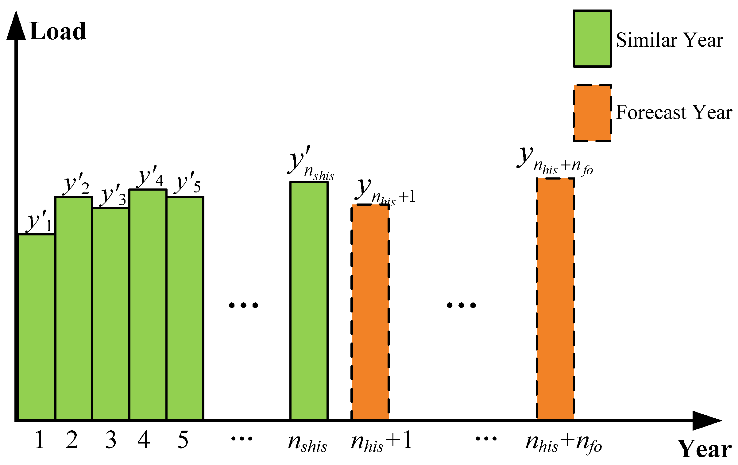
2. Similar Years Selection
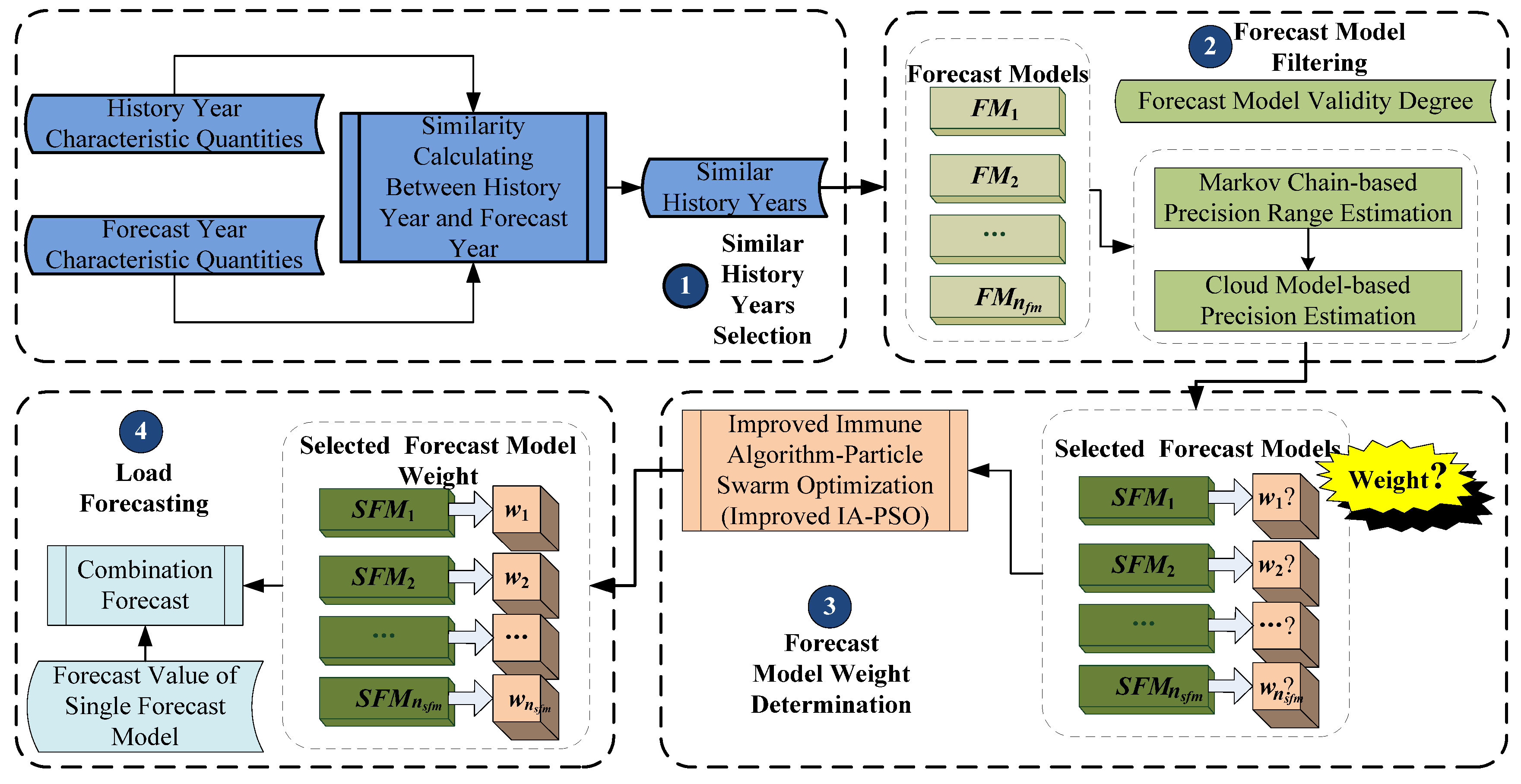
3. Forecast Model Filtering
3.1. Forecast Model Validity Degree

3.2. Forecast Model Precision Estimation
3.2.1. Markov Chain-Based Precision Range Estimation
3.2.2. Cloud Model-Based Precision Estimation
3.3. Forecast Model Filtering Based on Comprehensive Validity Degree
4. Forecast Model Weight Determination and Combination Forecast
4.1. Mathematical Description
4.2. Improved Immune Algorithm-Particle Swarm Optimization (Improved IA-PSO)
4.2.1. Particle Swarm Optimization (PSO)
- The momentum part represents the trust in its current motion state where w is the inertia coefficient used to control the influence of the speed on the speed . This part provides a necessary momentum which enables the particle to carry on the inertia motion based on its speed.
- The individual cognitive part represents the particle self-thinking behavior. This part encourages the particle to fly to the best position found by itself.
- The social cognitive part represents the information sharing and cooperation of different particles. This part guides the particle to fly to the best position of the group.
4.2.2. Immune Algorithm-Particle Swarm Optimization (IA-PSO)
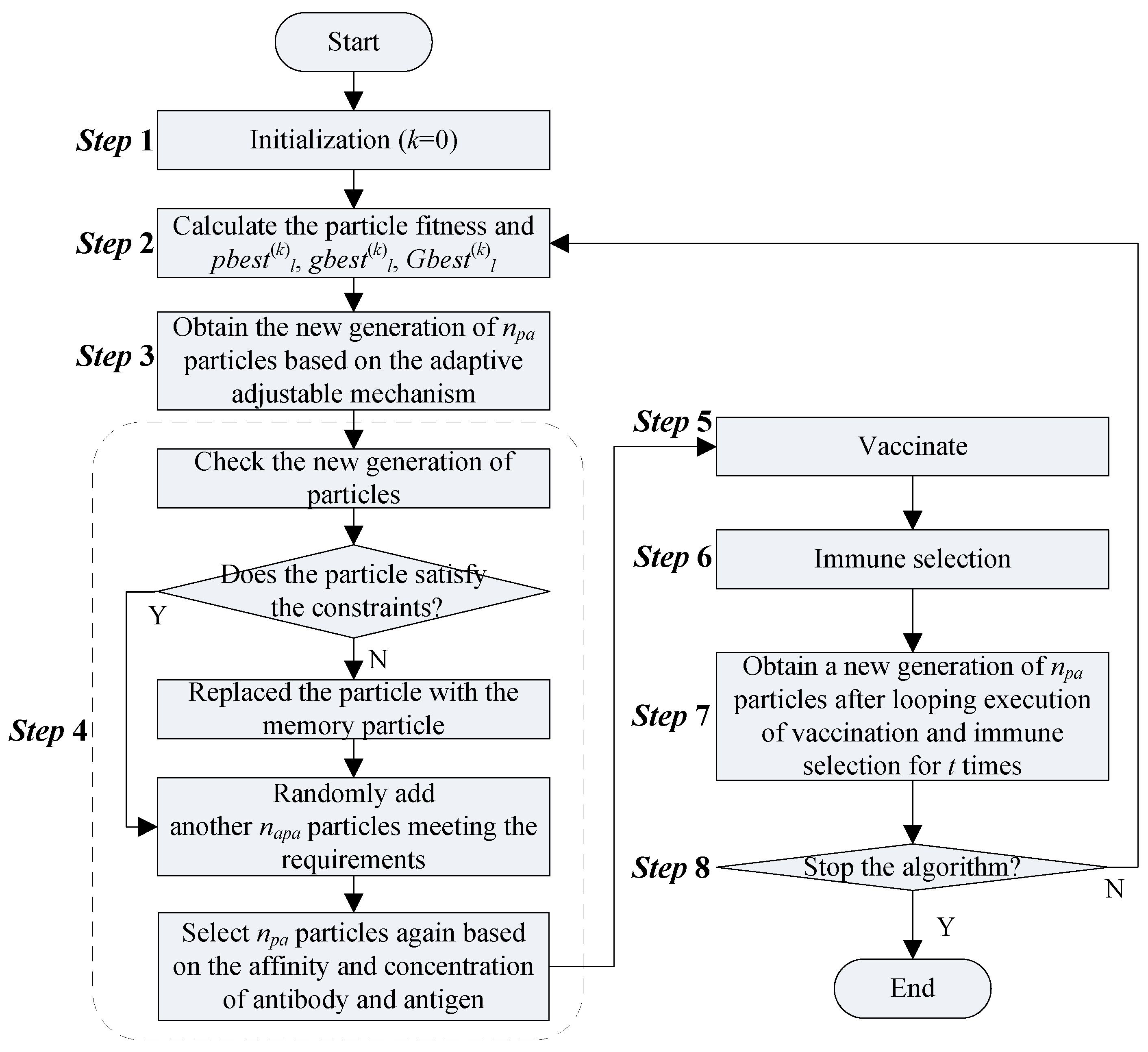
- Immune memory: The immune system keeps the antibodies opposing against the invading antigen as memory cells. If the same antigen invades again, the memory cells will be activated and produce a large number of antibodies. In IA-PSO, this idea is used to preserve the excellent particle. The best position searched by each particle up to now is considered as a memory cell. If the new born particles are detected not to meet the requirements, they will be replaced by the memory cells.
- Immune regulation: In IA-PSO, immune regulation is used for particle selection. If a particle has a strong affinity or a low concentration, it will be promoted. Otherwise, it will be demoted. Therefore, the particle diversification can be always kept. The selected probability [48,49] of the particle PAl is as follows:In Equation (28), represents the selected probability determined by the affinity where AFl is the affinity of the particle PAl, represents the selected probability determined by the concentration where CONl is the concentration of the particle PAl. χ represents the weight of PROl1 and 1 − χ represents the weight of PROl2 (0 ≤ χ ≤ 1).
- Immune selection: In the immune system, vaccinating means to change several components of the antibody according to the vaccination. In IA-PSO, the group best position up to the iteration iterk can be considered as the closest one to the optimal solution. Thus, we use several components of as the vaccination to vaccinate the particles and calculate the particle fitness value for immune selection. If the particle fitness value after the vaccination is lower than its parent, the vaccination will be abolished. Otherwise, the particle will be retained.
4.2.3. Improved IA-PSO Based on Disturbance Variable
Introducing Disturbance Variable into IA-PSO
Establishing the Adaptive Adjustable Strategy of Particle Searching Speed
4.3. Implementation Steps of Forecast Model Weight Determination Based on Improved IA-PSO

4.4. Weighted Combination Forecast
5. Case Study

| Year | Area GDP (108 Yuan) | Primary Industry GDP Ratio (%) | Secondary Industry GDP Ratio (%) | Tertiary Industry GDP Ratio (%) | Power Consumption per Unit of GDP (kWh/Yuan) | Electricity Price (Yuan/kWh) | Urban per-Capita Income (Yuan) | Rural per-Capita Income (Yuan) |
|---|---|---|---|---|---|---|---|---|
| 1998 | 9686.6 | 12.95 | 50.22 | 36.83 | 0.156 | 0.408 | 3005.21 | 1896.56 |
| 1999 | 9802.8 | 12.90 | 49.90 | 37.20 | 0.152 | 0.408 | 3859.86 | 2003.63 |
| 2000 | 9912.3 | 12.88 | 50.07 | 37.05 | 0.150 | 0.410 | 4663.23 | 2150.36 |
| 2001 | 10,626.6 | 12.83 | 50.06 | 37.11 | 0.148 | 0.412 | 5551.91 | 2340.14 |
| 2002 | 11,586.5 | 12.80 | 49.69 | 37.51 | 0.142 | 0.412 | 6599.24 | 2485.86 |
| 2003 | 12,955.2 | 12.38 | 50.75 | 36.87 | 0.139 | 0.412 | 7370.65 | 2657.93 |
| 2004 | 15,133.9 | 12.68 | 51.63 | 35.69 | 0.132 | 0.419 | 8245.55 | 3103.98 |
| 2005 | 17,140.8 | 12.79 | 49.62 | 37.59 | 0.125 | 0.444 | 9227.55 | 3391.82 |
| Year | Cosine Similarity (%) |
|---|---|
| 1998 | 98.56 |
| 1999 | 95.21 |
| 2000 | 94.66 |
| 2001 | 99.60 |
| 2002 | 97.52 |
| 2003 | 96.37 |
| 2004 | 98.63 |
| Year | 1998 | 2001 | 2002 | 2003 | 2004 | 2005 |
|---|---|---|---|---|---|---|
| Power Consumption | 437.85 | 557.58 | 628.82 | 725.20 | 833.01 | 946.33 |
| Forecast Model | 1998 | 2001 | 2002 | 2003 | 2004 | 2005 |
|---|---|---|---|---|---|---|
| FM1: Exponential model (y = 780.65e−0.82/x) | 343.91 | 636.02 | 662.58 | 680.93 | 694.36 | 704.55 |
| FM2: Logarithm model (y = 362.13 + 188.39lnx) | 362.09 | 623.33 | 665.32 | 699.65 | 728.73 | 753.90 |
| FM3: Hyperbola model (y = 722.84 − 354.37/x) | 368.54 | 634.24 | 652.01 | 663.76 | 672.21 | 678.53 |
| FM4: Para-curve model (y = 431.79 − 3.58x + 8.17x2) | 436.88 | 556.81 | 631.53 | 723.67 | 833.29 | 960.30 |
| FM5:Grey system method [53] | 437.94 | 567.04 | 642.01 | 727.00 | 823.23 | 932.08 |
| FM6: COMPERTZ model (lny = 6.46 − 1.29e−x) | 400.04 | 626.88 | 636.27 | 639.75 | 641.14 | 641.64 |
| FM7: Power function model (y = 358.90x0.385) | 358.90 | 612.43 | 667.48 | 716.12 | 759.91 | 800.02 |
| FM8: Cubic curve model (y = 432.10 − 3.94x + 8.81x2 − 0.0087x3) | 437.04 | 556.81 | 631.56 | 723.84 | 833.17 | 960.04 |
| FM9: Artificial neural network method [36] | 406.81 | 583.02 | 658.81 | 725.38 | 775.44 | 809.03 |
| FM10: S-curve model (y−1 = 0.0015 + 0.0039e−x) | 345.60 | 649.47 | 669.01 | 676.35 | 679.22 | 680.30 |
| FM11: Exponential smoothing method [54] | 437.85 | 544.91 | 615.01 | 708.33 | 816.72 | 892.51 |
| Forecast Model | Comprehensive Validity Degree (%) |
|---|---|
| FM1 | 81.09 |
| FM2 | 77.90 |
| FM3 | 75.56 |
| FM4 | 84.32 |
| FM5 | 85.80 |
| FM6 | 79.03 |
| FM7 | 74.87 |
| FM8 | 88.91 |
| FM9 | 87.23 |
| FM10 | 78.45 |
| FM11 | 82.91 |
| Algorithm | Iteration Number | The Forecast Model Weight | ||||
|---|---|---|---|---|---|---|
| SFM1 | SFM2 | SFM3 | SFM4 | SFM5 | ||
| FMWD-PSO | 623 | 0.0611 | 0.2120 | 0.3876 | 0.0861 | 0.2532 |
| FMWD-IA-PSO | 490 | 0.2598 | 0.1662 | 0.3343 | 0.0343 | 0.2054 |
| FMWD-improved-IA-PSO | 193 | 0.4105 | 0.0401 | 0.4895 | 0.0002 | 0.0597 |
| Weighted Combination Forecast | 1998 | 2001 | 2002 | 2003 | 2004 | 2005 |
|---|---|---|---|---|---|---|
| WCF-FMWD-PSO | 434.82 | 558.22 | 631.93 | 720.71 | 821.93 | 923.03 |
| WCF-FMWD-IA-PSO | 436.28 | 556.97 | 630.82 | 721.19 | 826.19 | 936.41 |
| WCF-FMWD-improved-IA-PSO | 437.05 | 556.52 | 630.98 | 722.97 | 831.81 | 954.96 |
| Forecast Method | Mean Absolute Percentage Error (%) | Percentage Error (%) | |||||
|---|---|---|---|---|---|---|---|
| 1998 | 2001 | 2002 | 2003 | 2004 | 2005 | ||
| SFM1 | 0.42 | −0.22 | −0.14 | 0.43 | −0.21 | 0.03 | 1.48 |
| SFM2 | 1.12 | 0.02 | 1.70 | 2.10 | 0.25 | 1.17 | −1.51 |
| SFM3 | 0.40 | −0.18 | −0.14 | 0.44 | −0.19 | 0.02 | 1.45 |
| SFM4 | 6.31 | −7.09 | 4.56 | 4.77 | 0.02 | −6.91 | −14.51 |
| SFM5 | 2.41 | 0 | −2.27 | −2.20 | −2.33 | −1.96 | −5.69 |
| Equal weight method [55] | 0.98 | 0.04 | 1.56 | 1.10 | 0.80 | −1.02 | −1.33 |
| Variance analysis method [55] | 1.25 | 0.02 | −1.27 | −0.20 | −2.21 | −1.16 | −2.63 |
| Optimum fitting method [55] | 2.78 | −2.09 | 5.56 | 0.77 | 1.02 | −2.91 | −4.32 |
| Optimum forecast method [55] | 1.16 | −0.59 | 2.11 | 0.97 | 0.56 | 1.21 | 1.50 |
| WCF-FMWD-PSO | 0.93 | −0.69 | 0.12 | 0.49 | −0.62 | −1.33 | −2.36 |
| WCF-FMWD-IA-PSO | 0.53 | −0.36 | −0.11 | 0.32 | −0.55 | −0.82 | −1.05 |
| WCF-FMWD-improved-IA-PSO | 0.35 | −0.18 | −0.19 | 0.34 | −0.31 | −0.14 | 0.91 |
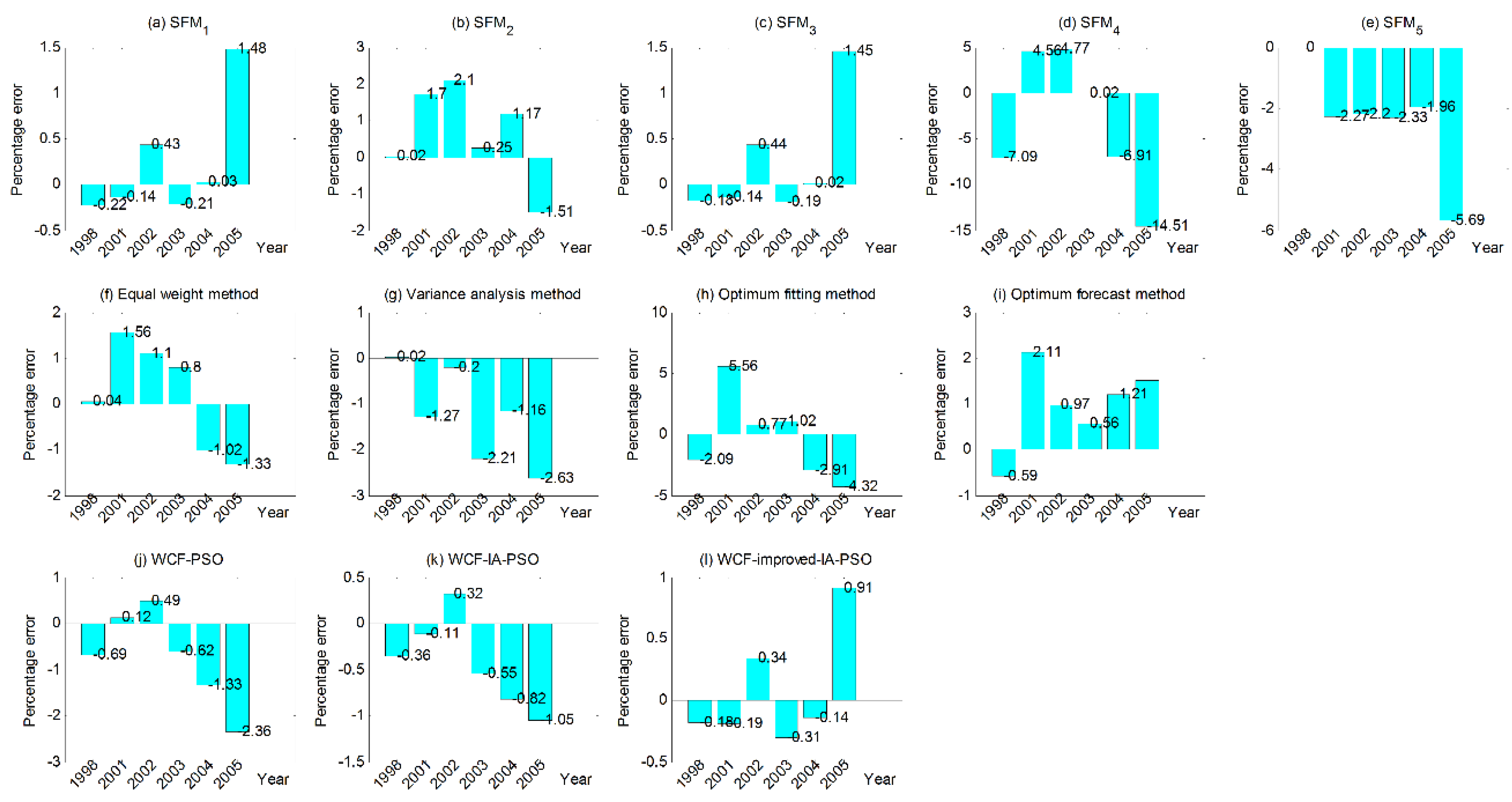
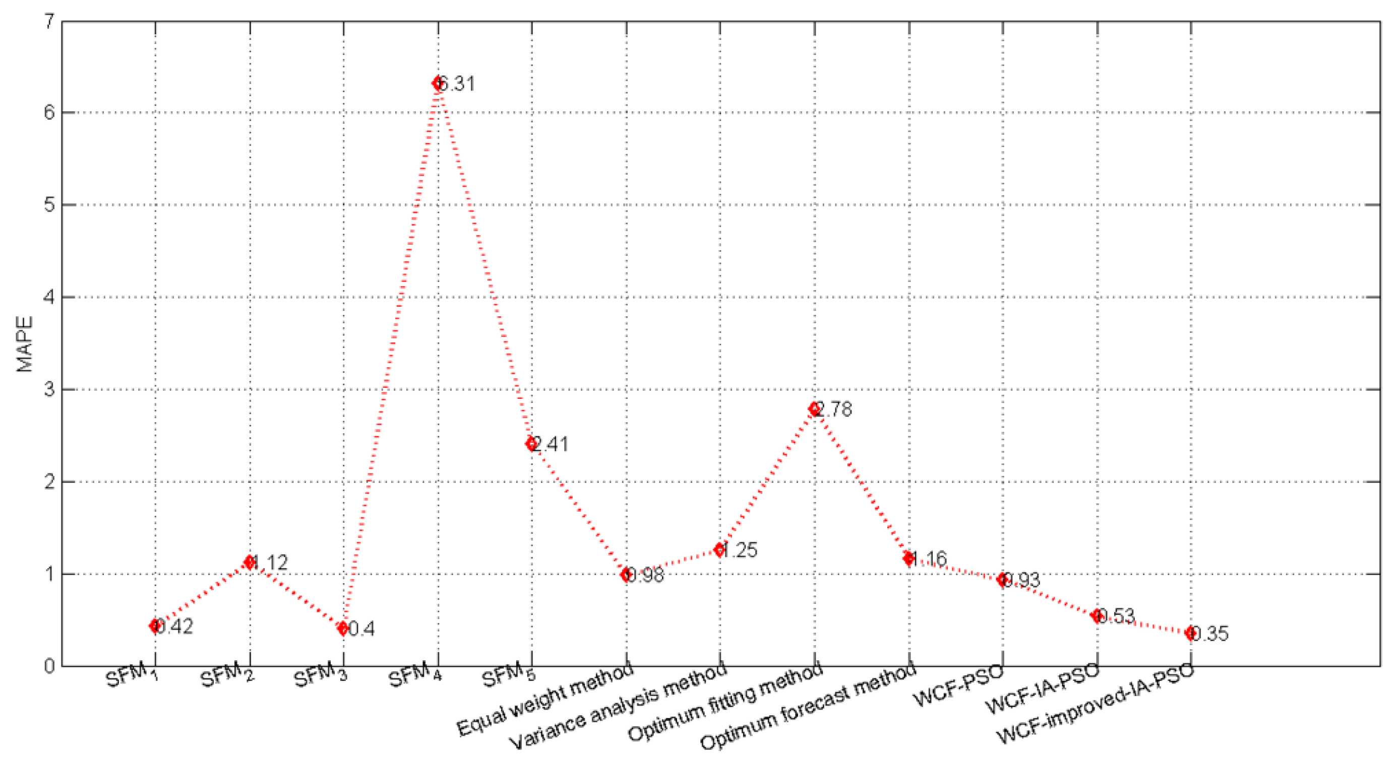
- The maximum and minimum PE of the single forecast models (SFM1–SFM5) are −14.51% and 0 respectively, the maximum and minimum MAPE of the single forecast models (SFM1–SFM5) are 6.31% and 0.40% respectively.
- The maximum and minimum PE of WCF-FMWD-PSO are −2.36% and 0.12% respectively, the MAPE of WCF-FMWD-PSO is 0.93% and the iteration number is 623.
- The maximum and minimum PE of WCF-FMWD-IA-PSO are 1.05% and −0.11% respectively, the MAPE of WCF-FMWD-IA-PSO is 0.53% and the iteration number is 490.
- The maximum and minimum PE of WCF-FMWD-improved-IA-PSO are 0.91% and −0.14% respectively, the MAPE of WCF-FMWD-improved-IA-PSO is 0.35% and the iteration number is 193.

6. Conclusions
- (1)
- Due to the fact that the forecast year’s true load is unknown, the comprehensive validity degree of forecast model is defined by the integration of fitted value relative error and forecast value relative error, and then forecast models are filtered based on their comprehensive validity degrees.
- The definition of validity degree can effectively overcome the inherent shortcomings of error theory. Entirely investigating the fitting level and the validity of forecast model, the comprehensive validity degree definition and the forecast model filtering method can improve the robustness of combination forecasting.
- Revealing the transition pattern between the natural precision and validity degree, the forecast precision estimation method based on Markov chain and cloud model can provide an important basis for the subsequent weighted combination forecasting. In the forecast models’ filtering, the better ones will be selected and the worse ones will be eliminated. It can also improve the robustness of combination forecasting.
- (2)
- The improved IA-PSO is used to determine the forecast model weight in combination forecasting. Based on the uniting of immune system’s specific information processing mechanism and PSO’s global convergence ability, disturbance variable and particle searching speed’s adaptive adjustable strategy are introduced to improve the algorithm performance. The particles’ diversity is ensured while the convergence speed is increased. It can avoid the local optimal and improve the accuracy.
Acknowledgments
Author Contributions
Conflicts of Interest
Nomenclature
| n | number |
| CH | year characteristic |
| CHQ | year characteristic quantity |
| HY | history year |
| FY | forecast year |
| CSI | Cosine similarity |
| FM | forecast model |
| y′ | similar year load |
| y | forecast year load |
| y‴ | forecast year load by a forecast model |
| RE′ | fitted value relative error |
| RE | forecast value relative error |
| P′ | fitted precision |
| P | forecast precision |
| FIV | fitted validity degree |
| FOV | forecast validity degree |
| S | sub-interval |
| OC | occurrence number |
| TRN | transition number |
| TP | transition probability |
| TM | state transition matrix |
| IV | initial vector |
| SM | state matrix |
| CVE | column vector |
| Ex | expectation |
| En | entropy |
| He | hyper-entropy |
| En′ | normal random number |
| CV | comprehensive validity degree |
| SFM | selected forecast model |
| PO | particle swarm |
| PA | particle |
| x | position |
| v | speed |
| LF | learning factor |
| rand | random number |
| w | inertia coefficient |
| PRO | probability |
| AF | affinity |
| CON | concentration |
| iter | iteration |
| F | fitness function |
| PF | particle fitness |
| r | vaccination times |
| Var | variance |
| Dev | deviation |
| Greek letters | |
| σ | standard deviation |
| α | empirical coefficient |
weight | |
disturbance variable | |
swarm convergence degree | |
coefficient used to control the upper limit | |
| ω | forecast model’s weight |
| Superscripts | |
| g | the gth sub-interval |
| h | the hth sub-interval |
| (h, g) | the transition from the hth to the gth |
| (k) | the kth iteration |
| (q) | step |
| q | the qth power |
| Subscripts | |
| his | history year |
| fo | forecast year |
| shis | selected history year |
| fm | forecast model |
| sfm | selected forecast model |
| si | sub-interval |
| pa | particle |
| apa | added particle |
| avg | average |
| AVG | the average of the numbers which are bigger than the global average |
| a | the ath year characteristic |
| b | the bth year characteristic quantity |
| c | the cth forecast year |
| d | the dth forecast model |
| e | the eth similar year |
| i | the ith column vector |
| j | the jth selected forecast model |
| l | the lth particle |
| m | the dimensional number of solution space |
| t | the tth element |
References
- Kouhi, S.; Keynia, F. A new cascade NN based method to short-term load forecast in deregulated electricity market. Energy Convers. Manag. 2013, 71, 76–83. [Google Scholar] [CrossRef]
- Chaturvedi, D.K.; Sinha, A.P.; Malik, O.P. Short term load forecast using fuzzy logic and wavelet transform integrated generalized neural network. Int. J. Electr. Power Energy Syst. 2015, 67, 230–237. [Google Scholar] [CrossRef]
- Yang, Z.C. Electric load evaluation and forecast based on the elliptic orbit algorithmic model. Int. J. Electr. Power Energy Syst. 2012, 42, 560–567. [Google Scholar]
- Bennett, C.; Stewart, R.A.; Lu, J. Autoregressive with exogenous variables and neural network short-term load forecast models for residential low voltage distribution networks. Energies 2014, 7, 2938–2960. [Google Scholar] [CrossRef]
- Li, F.; Buxiang, Z.; Shi, C. The Medium and Long Term Load Forecasting Combined Model Considering Weight Scale Method. TELKOMNIKA Indones. J. Electr. Eng. 2013, 11, 2181–2186. [Google Scholar] [CrossRef]
- Li, R.; Su, H.; Wang, Z. Medium-and long-term load forecasting based on heuristic least square support vector machine. Power Syst. Technol. 2011, 35, 195–199. (In Chinese) [Google Scholar]
- Mello, P.E.; Lu, N.; Makarov, Y. An optimized autoregressive forecast error generator for wind and load uncertainty study. Wind Energy 2011, 14, 967–976. [Google Scholar] [CrossRef]
- Li, H.; Guo, S.; Zhao, H. Annual electric load forecasting by a least squares support vector machine with a fruit fly optimization algorithm. Energies 2012, 5, 4430–4445. [Google Scholar] [CrossRef]
- Filik, Ü.B.; Gerek, Ö.N.; Kurban, M. A novel modeling approach for hourly forecasting of long-term electric energy demand. Energy Convers. Manag. 2011, 52, 199–211. [Google Scholar] [CrossRef]
- Suganthi, L.; Samuel, A.A. Energy models for demand forecasting—A review. Renew. Sustain. Energy Rev. 2012, 16, 1223–1240. [Google Scholar] [CrossRef]
- Sheikh, S.K.; Unde, M.G. Short Term Load Forecasting using ANN Technique. Int. J. Eng. Sci. Emerg. Technol. 2012, 1, 97–107. [Google Scholar]
- Wu, Y. The medium and long-term load forecasting based on improved D-S evidential theory. Trans. China Electrotech. Soc. 2012, 27, 157–162. (In Chinese) [Google Scholar]
- Long, R.; Mao, Y.; Mao, L. A combination model for medium-and long-term load forecasting based on induced ordered weighted averaging operator and Markov chain. Power Syst. Technol. 2010, 3, 150–156. (In Chinese) [Google Scholar]
- Chen, H.Y. The Validity Theory of Combination Forecasting Method and Its Application; Science Press: Beijing, China, 2008; pp. 76–109. (In Chinese) [Google Scholar]
- Chen, H.Y. Research on combination forecasting model based on effective measure of forecasting methods. Forecasting 2001, 20, 72–73. [Google Scholar]
- Sun, G.Q.; Yao, J.G.; Xie, Y.X. Combination forecast of medium-and-long-term load using fuzzy adaptive variable weight based on fresh degree function and forecasting availability. Power Syst. Technol. 2009, 33, 103–107. (In Chinese) [Google Scholar]
- Chen, C.; Guo, W.; Fan, J.Z. Combined method of mid-long term load forecast based on improved forecasting effectiveness. Relay 2007, 35, 70–74. (In Chinese) [Google Scholar]
- Jin, X.; Luo, D.S.; Sun, G.Q. Sifting and combination method of medium-and-long-term load forecasting model. Proc. Chin. Soc. Univ. Electr. Power Syst. Autom. 2012, 24, 150–156. (In Chinese) [Google Scholar]
- Hernandez, L.; Baladrón, C.; Aguiar, J.M. Short-term load forecasting for microgrids based on artificial neural networks. Energies 2013, 6, 1385–1408. [Google Scholar] [CrossRef]
- Gofman, A.V.; Vedernikov, A.S.; Vedernikova, E.S. Increasing the accuracy of the short-term and operational prediction of the load of a power system using an artificial neural network. Power Technol. Eng. 2013, 46, 410–415. [Google Scholar] [CrossRef]
- Li, H.; Guo, S.; Li, C. A hybrid annual power load forecasting model based on generalized regression neural network with fruit fly optimization algorithm. Knowledge-Based Syst. 2013, 37, 378–387. [Google Scholar] [CrossRef]
- Paparoditis, E.; Sapatinas, T. Short-term load forecasting: The similar shape functional time-series predictor. IEEE Trans. Power Syst. 2013, 28, 3818–3825. [Google Scholar] [CrossRef]
- Weron, R.; Taylor, J. Discussion on “Electrical load forecasting by exponential smoothing with covariates”. Appl. Stoch. Models Bus. Ind. 2013, 29, 648–651. [Google Scholar] [CrossRef]
- Li, D.C.; Chang, C.J.; Chen, C.C. Forecasting short-term electricity consumption using the adaptive grey-based approach—An Asian case. Omega 2012, 40, 767–773. [Google Scholar] [CrossRef]
- Ismail, N.A.; King, M. Factors influencing the alignment of accounting information systems in small and medium sized Malaysian manufacturing firms. J. Inf. Syst. Small Bus. 2014, 1, 1–20. [Google Scholar]
- Kodogiannis, V.S.; Amina, M.; Petrounias, I. A clustering-based fuzzy wavelet neural network model for short-term load forecasting. Int. J. Neural Syst. 2013, 23, 1557–1565. [Google Scholar] [CrossRef] [PubMed]
- Hong, T.; Wang, P. Fuzzy interaction regression for short term load forecasting. Fuzzy Optim. Decis. Mak. 2014, 13, 91–103. [Google Scholar] [CrossRef]
- Borges, C.E.; Penya, Y.K.; Fernandez, I. Evaluating combined load forecasting in large power systems and smart grids. IEEE Trans. Ind. Inf. 2013, 9, 1570–1577. [Google Scholar] [CrossRef]
- Che, J.; Wang, J.; Wang, G. An adaptive fuzzy combination model based on self-organizing map and support vector regression for electric load forecasting. Energy 2012, 37, 657–664. [Google Scholar] [CrossRef]
- Liu, Z.; Li, W.; Sun, W. A novel method of short-term load forecasting based on multiwavelet transform and multiple neural networks. Neural Comput. Appl. 2013, 22, 271–277. [Google Scholar] [CrossRef]
- Wang, J.; Wang, J.; Li, Y. Techniques of applying wavelet de-noising into a combined model for short-term load forecasting. Int. J. Electr. Power Energy Syst. 2014, 62, 816–824. [Google Scholar] [CrossRef]
- Enayatifar, R.; Sadaei, H.J.; Abdullah, A.H. Imperialist competitive algorithm combined with refined high-order weighted fuzzy time series (RHWFTS-ICA) for short term load forecasting. Energy Convers. Manag. 2013, 76, 1104–1116. [Google Scholar] [CrossRef]
- Ko, C.N.; Lee, C.M. Short-term load forecasting using SVR (support vector regression)-based radial basis function neural network with dual extended Kalman filter. Energy 2013, 49, 413–422. [Google Scholar] [CrossRef]
- Ma, S.; Chen, X.; Liao, Y.; Wang, G.; Ding, X.; Chen, K. The variable weight combination load forecasting based on grey model and semi-parametric regression model. In Proceedings of the TENCON 2013—2013 IEEE Region 10 Conference (31194), Xi’an, China, 22–25 October 2013; pp. 1–4.
- Niu, D.; Shi, H.; Wu, D.D. Short-term load forecasting using bayesian neural networks learned by Hybrid Monte Carlo algorithm. Appl. Soft Comput. 2012, 12, 1822–1827. [Google Scholar] [CrossRef]
- Zhu, J.P.; Dai, J. Optimization selection of correlative factors for long-term load prediction of electric power. Comput. Simul. 2008, 5, 226–229. [Google Scholar]
- Wang, Q.; Wang, Y.L.; Zhang, L.Z. An approach to allocate impersonal weights of factors influencing electric power demand forecasting. Power Syst. Technol. 2008, 32, 82–86. (In Chinese) [Google Scholar]
- Lei, S.L.; Gu, L.; Yang, J.; Liu, X.Y. Analysis of electric power load characteristics and its influencing factors in chongqing region. Electr. Power 2014, 12, 61–71. (In Chinese) [Google Scholar]
- Liao, F.; Congying, X.U.; Yao, J.; Cai, J.; Chen, S. Load characteristics of change region and analysis on its influencing factors. Power Syst. Technol. 2012, 7, 117–125. [Google Scholar]
- Karakoc, E.; Cherkasov, A.; Sahinalp, S.C. Distance based algorithms for small biomolecule classification and structural similarity search. Bioinformatics 2006, 14, 243–251. [Google Scholar] [CrossRef] [PubMed]
- Ye, J. Cosine similarity measures for intuitionistic fuzzy sets and their applications. Math. Comput. Model. 2011, 1, 91–97. [Google Scholar] [CrossRef]
- Zhu, S.; Wu, J.; Xiong, H.; Xia, G. Scaling up top-K cosine similarity search. Data Knowl. Eng. 2011, 1, 60–83. [Google Scholar] [CrossRef]
- Keilson, J. Markov Chain Models—Rarity and Exponentiality; Springer Science and Business Media: Berlin, Germany, 2012. [Google Scholar]
- Yoder, M.; Hering, A.S.; Navidi, W.C.; Larson, K. Short-term forecasting of categorical changes in wind power with Markov chain models. Wind Energy 2014, 17, 1425–1439. [Google Scholar] [CrossRef]
- Li, D.Y.; Liu, C.Y. Study on the universality of the normal cloud model. Eng. Sci. 2004, 6, 28–34. [Google Scholar]
- Wang, G.; Xu, C.; Li, D. Generic normal cloud model. Inf. Sci. 2014, 280, 1–15. [Google Scholar] [CrossRef]
- Kennedy, J. Particle swarm optimization. In Encyclopedia of Machine Learning; Springer Publishing Company: New York, NY, USA, 2010; pp. 760–766. [Google Scholar]
- Zhao, F.; Li, G.; Yang, C.; Abraham, A.; Liu, H. A human-computer cooperative particle swarm optimization based immune algorithm for layout design. Neurocomputing 2014, 132, 68–78. [Google Scholar] [CrossRef]
- Fu, X.; Li, A.; Wang, L.; Ji, C. Short-term scheduling of cascade reservoirs using an immune algorithm-based particle swarm optimization. Comput. Math. Appl. 2011, 6, 2463–2471. [Google Scholar] [CrossRef]
- Afshinmanesh, F.; Marandi, A.; Rahimi-Kian, A. A novel binary particle swarm optimization method using artificial immune system. In Proceedings of the International Conference on Computer as a Tool, EUROCON 2005, Belgrade, Serbia, 21–24 November 2005; Volume 1, pp. 217–220.
- Wu, J.M.; Zuo, H.F.; Chen, Y. A combined forecasting method based on particle swarm optimization with immunity algorithms. Syst. Eng. Theory Method Appl. 2006, 15, 229–233. (In Chinese) [Google Scholar]
- China National Bureau of Statistics. China Energy Statistical Yearbook; China Statistics Press: Beijing, China, 2011. (In Chinese)
- Deng, J.L. Introduction to grey system theory. J. Grey Syst. 1989, 1, 1–24. (In Chinese) [Google Scholar]
- Gardner, E.S. Exponential smoothing: The state of the art. J. Forecast. 1985, 1, 1–28. [Google Scholar] [CrossRef]
- Kang, C.Q.; Xia, Q.; Liu, M. Power System Load Forecasting; China Electric Power Press: Beijing, China, 2007; pp. 73–75. (In Chinese) [Google Scholar]
© 2015 by the authors; licensee MDPI, Basel, Switzerland. This article is an open access article distributed under the terms and conditions of the Creative Commons by Attribution (CC-BY) license (http://creativecommons.org/licenses/by/4.0/).
Share and Cite
Li, L.; Mu, C.; Ding, S.; Wang, Z.; Mo, R.; Song, Y. A Robust Weighted Combination Forecasting Method Based on Forecast Model Filtering and Adaptive Variable Weight Determination. Energies 2016, 9, 20. https://doi.org/10.3390/en9010020
Li L, Mu C, Ding S, Wang Z, Mo R, Song Y. A Robust Weighted Combination Forecasting Method Based on Forecast Model Filtering and Adaptive Variable Weight Determination. Energies. 2016; 9(1):20. https://doi.org/10.3390/en9010020
Chicago/Turabian StyleLi, Lianhui, Chunyang Mu, Shaohu Ding, Zheng Wang, Runyang Mo, and Yongfeng Song. 2016. "A Robust Weighted Combination Forecasting Method Based on Forecast Model Filtering and Adaptive Variable Weight Determination" Energies 9, no. 1: 20. https://doi.org/10.3390/en9010020