
Optimal Allocation of Thermal-Electric Decoupling Systems Based on the National Economy by an Improved Conjugate Gradient Method

Abstract
:1. Introduction
2. The Thermal-Electric Coupling of TED and Its Decoupling
2.1. Thermal-Electric Coupling of TED
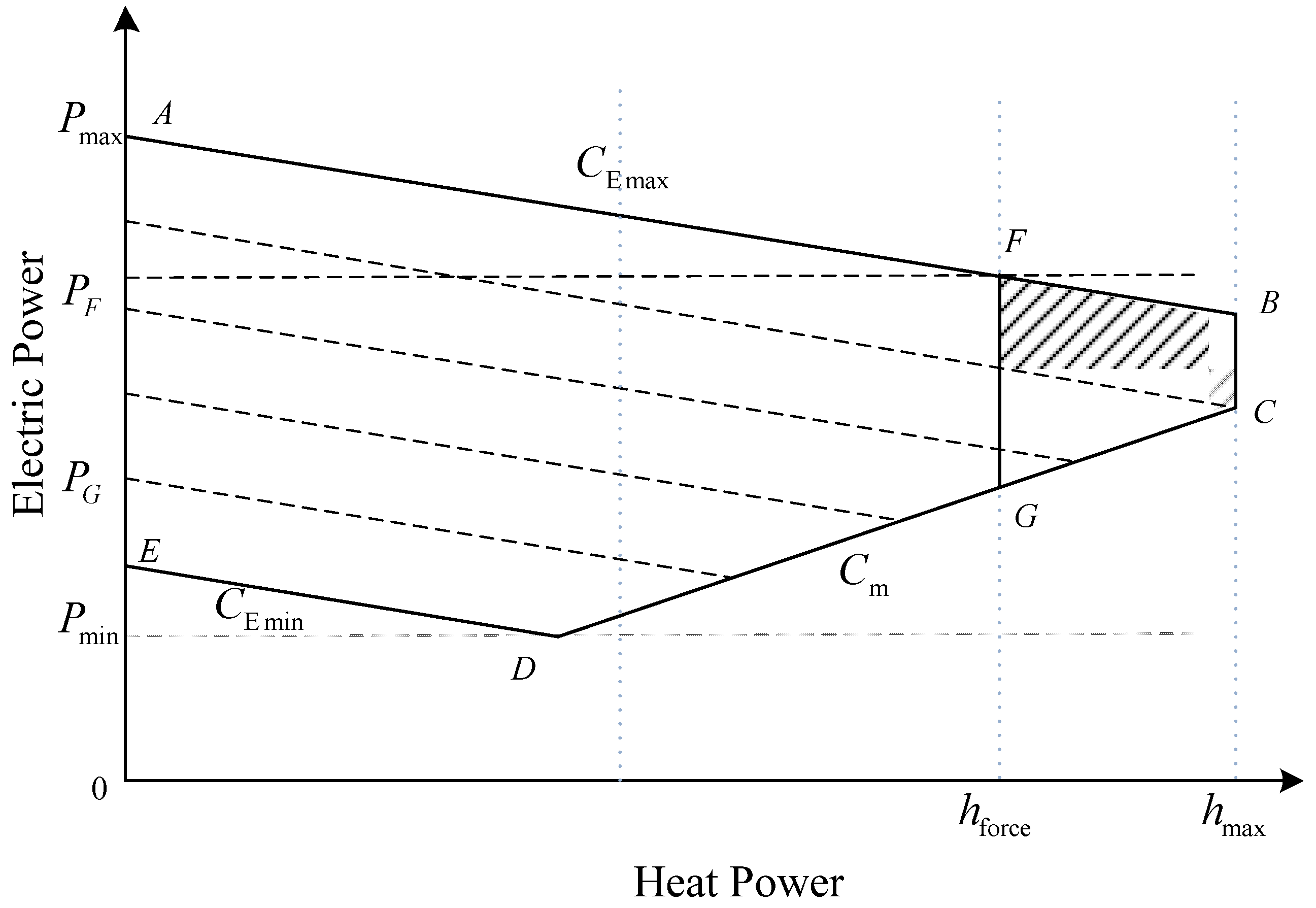
2.2. Principle of Thermal-Electric Decoupling
3. The Economic Analysis of the Application of TED
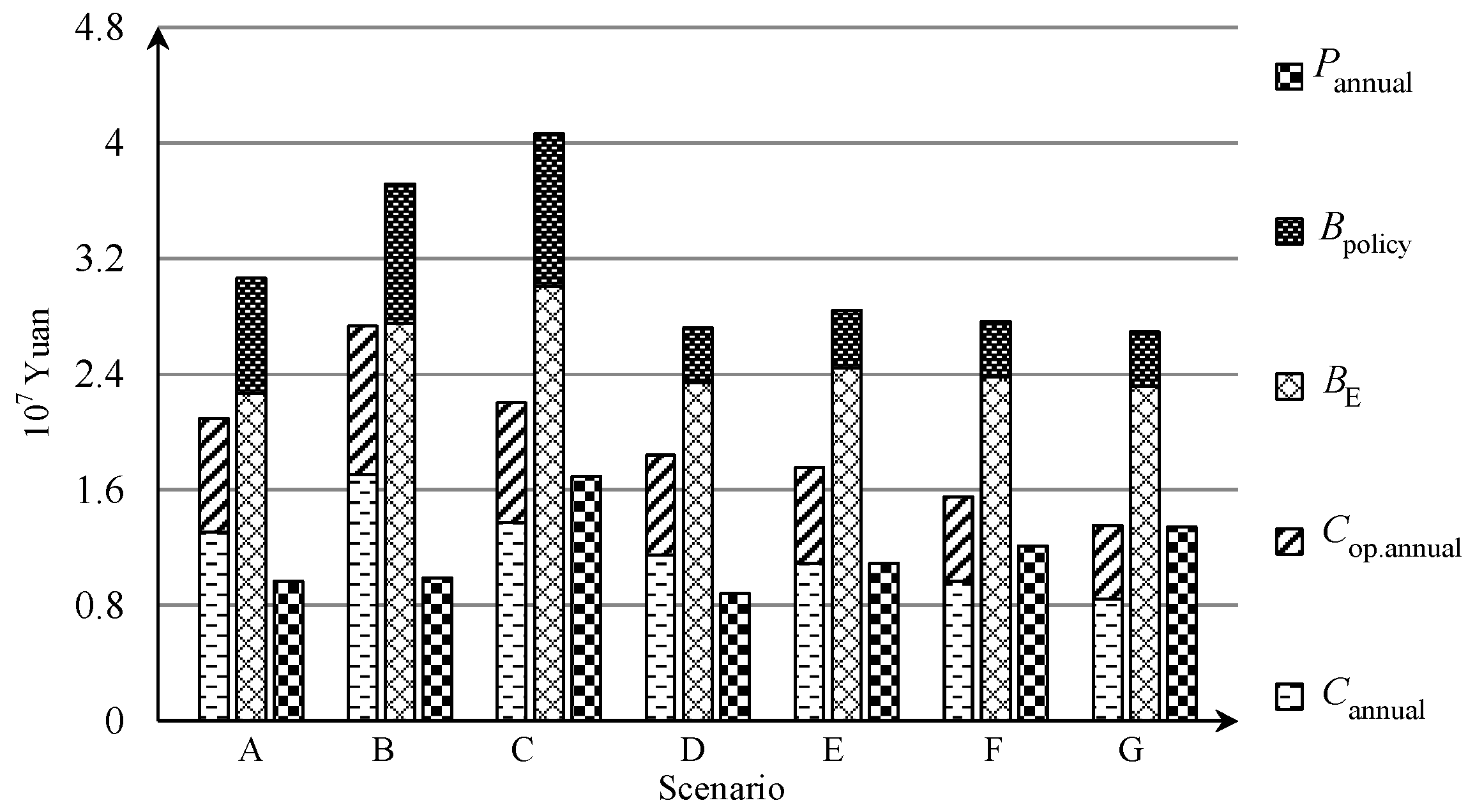
3.1. The Annual Income
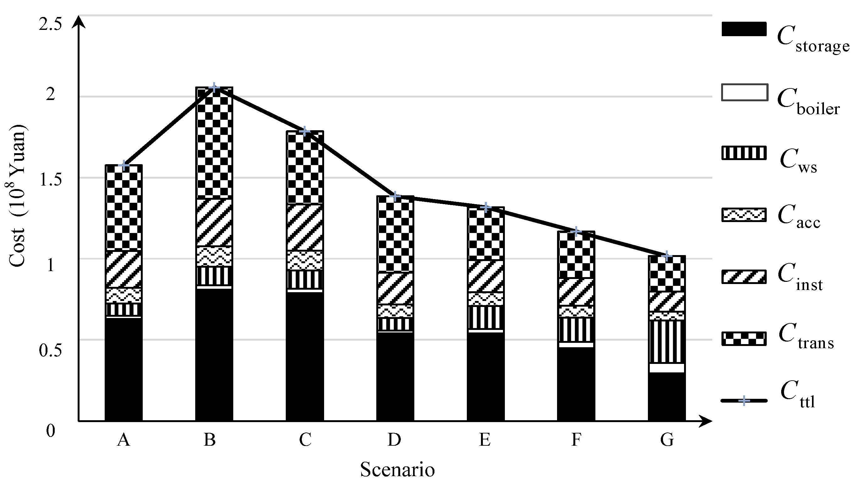
3.2. The Annual Cost during Design Lifetime
4. Constraint Conditions
4.1. Energy Balance Constraint
4.2. Electric Power Output and Heating Power Output Constraints
4.3. The Constraint of Thermal-Electric Output Coupling of CHPs
4.4. The Constraint of Unit Ramp Rate
4.5. The Constraint of TED Operation
5. Improved Parallel Conjugate Gradient Method
5.1. Unconstrained Optimization Algorithm
5.2. Parallel Computing Approach
5.3. Algorithm Calculating Procedures
- Step 1.
- Presenting an arbitrary initial value , set the initial direction:
- Step 2.
- If , calculate the eigenvalues of the Jacobian matrix. On condition that all of the eigenvalues are positive, the optimization converges to the optimum value and the optimal process could be stopped, while, in case of the existence of negative eigenvalues, it means the optimization converges to a saddle point ; in this condition the algorithm process shifts to Step 3. Else if , shift to Step 6.
- Step 3.
- Calculate all of the eigenvalues of the Jacobian matrix , … and the corresponding eigenvectors , ... , setting a new searching point:
- Step 4.
- For , if , it means the optimization is convergent, then judge the existence of a saddle point with the method mentioned in Step 2. If there is no saddle point, the optimization converges to the optimum value. If a saddle point could be detected, shift to Step 3 to re-set the new search point and a new direction. In case that , shift to Step 5.
- Step 5.
- Set a new search direction:
- Step 6.
- Set a new searching direction:
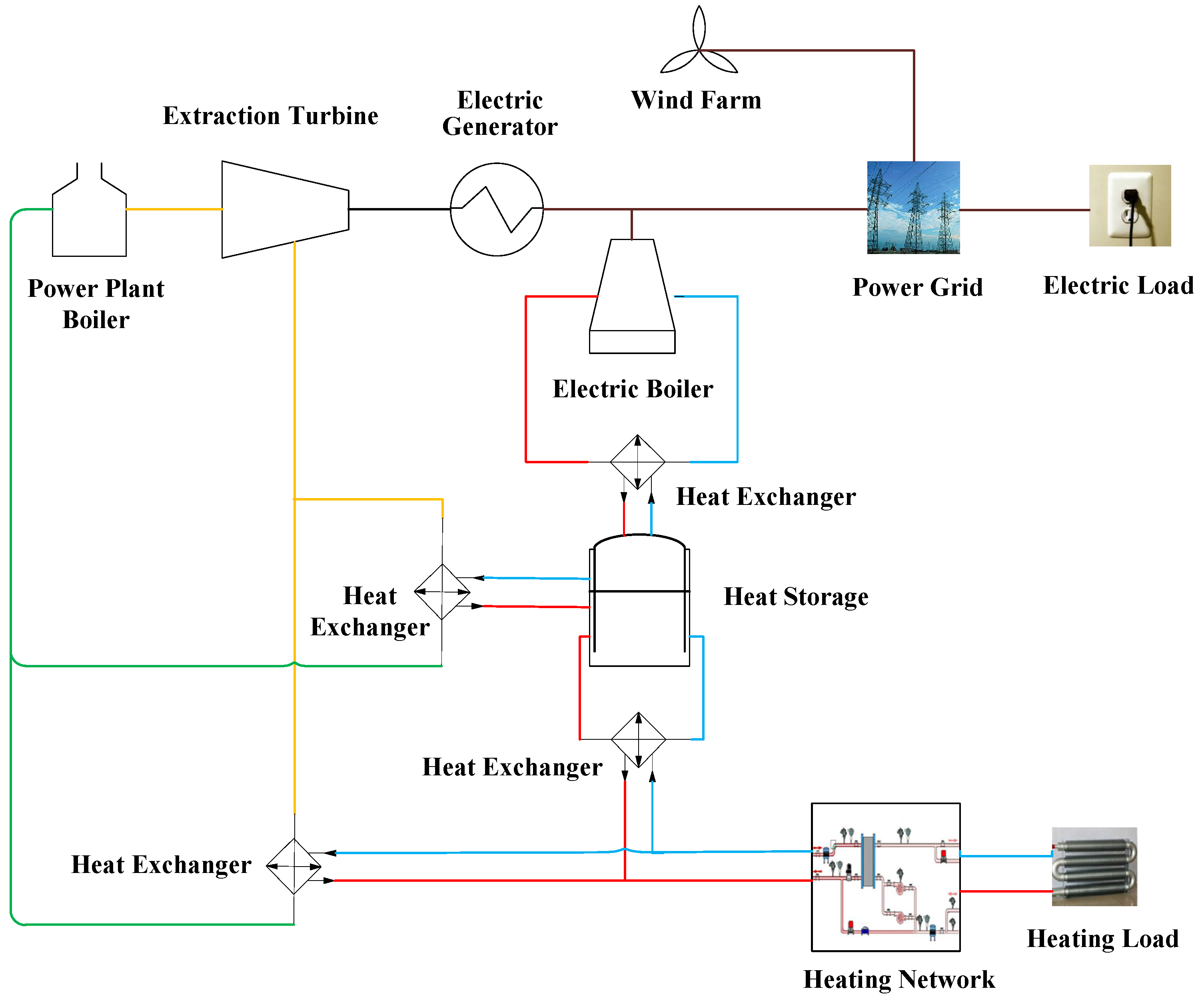
6. System Modeling and Numerical Simulation
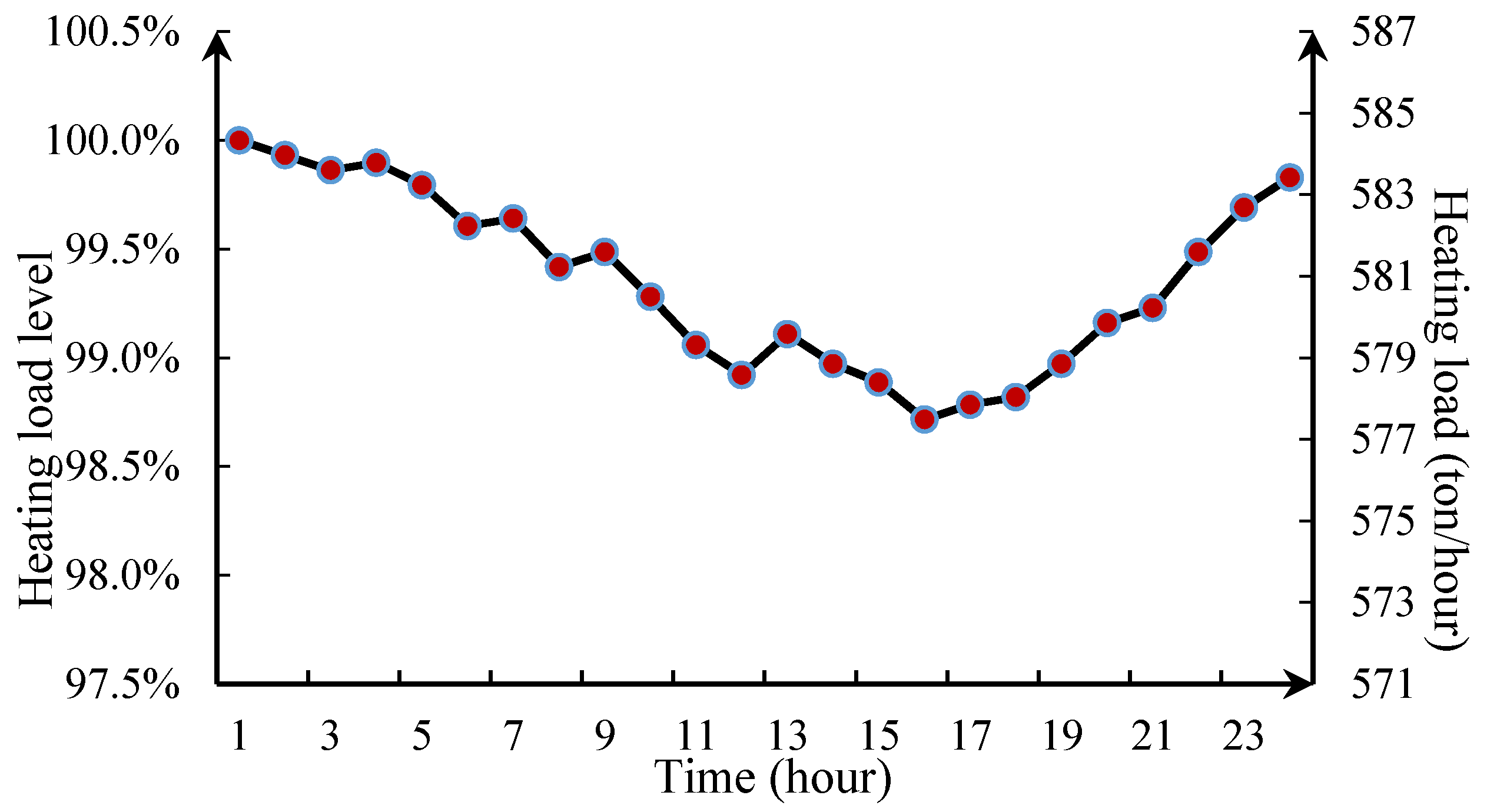
6.1. General Situation of Simulation

| Item | Value | Unit |
|---|---|---|
| Electric Boiler | 75 | 104 Yuan per MW |
| Heat Storage | 0.7 | 104 Yuan per m3 |
| Pumps | 0.4 | 104 Yuan per MW |
| Electric Power Transformer Equipment | 25 | 104 Yuan per MVA |
| Utility Building | 0.4 | 104 Yuan per m2 |
| Fuel | 0.065 | 104 Yuan per ton |
| Bank discount rate | 6.55 | % |
| Design service life | 20 | Year |
| Carbon trading price | 50 | Yuan per ton |
| Coal Evaluation on Electricity Generation | 0.1229 | ton per MWh |
| Coal Evaluation on Heat Generation | 0.03412 | tom per GJ |
| Heat Price | 21.5 | Yuan per GJ |
| Electricity Price | 386.4 | Yuan per MWh |
6.2. System Modeling


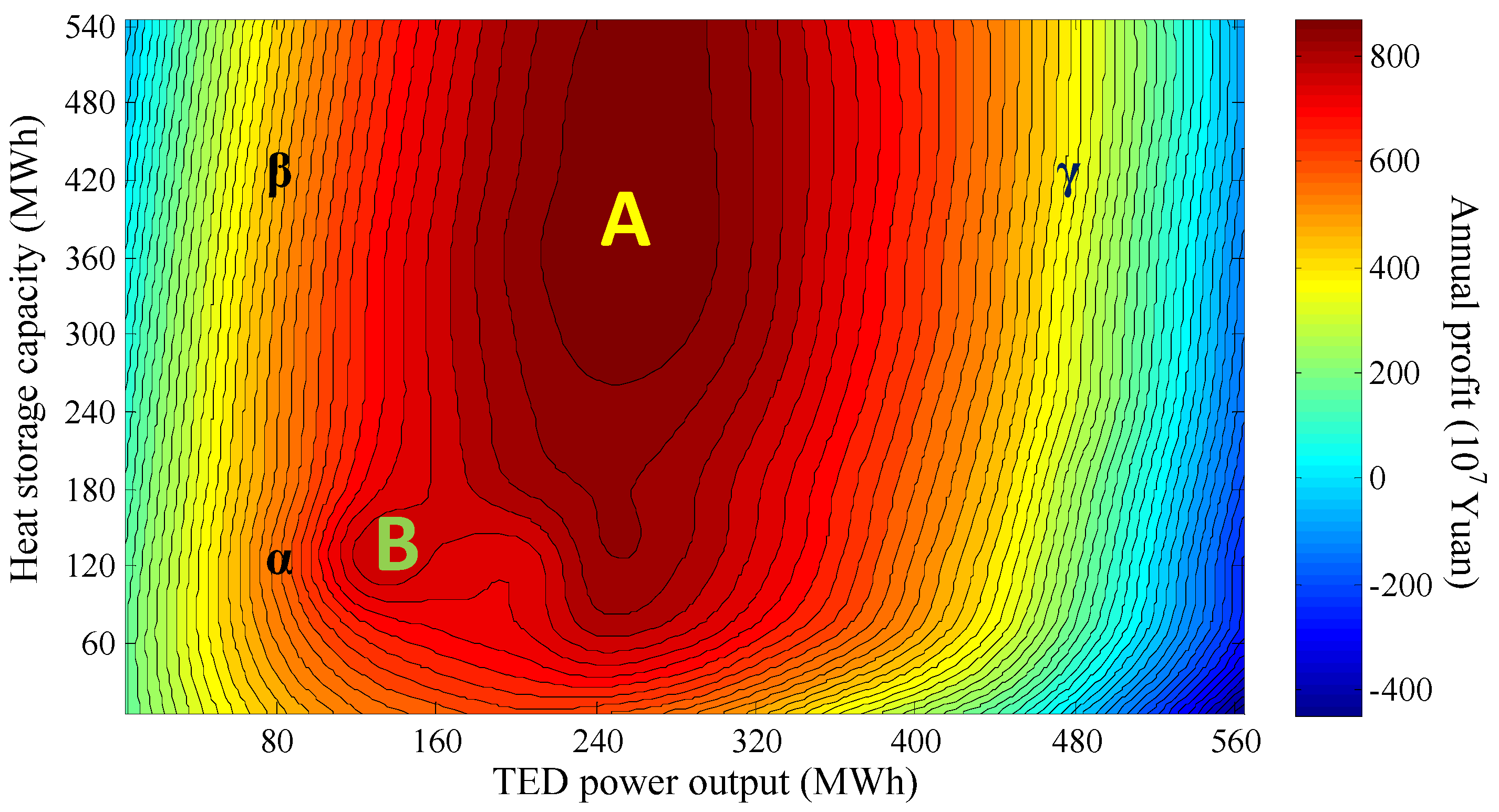
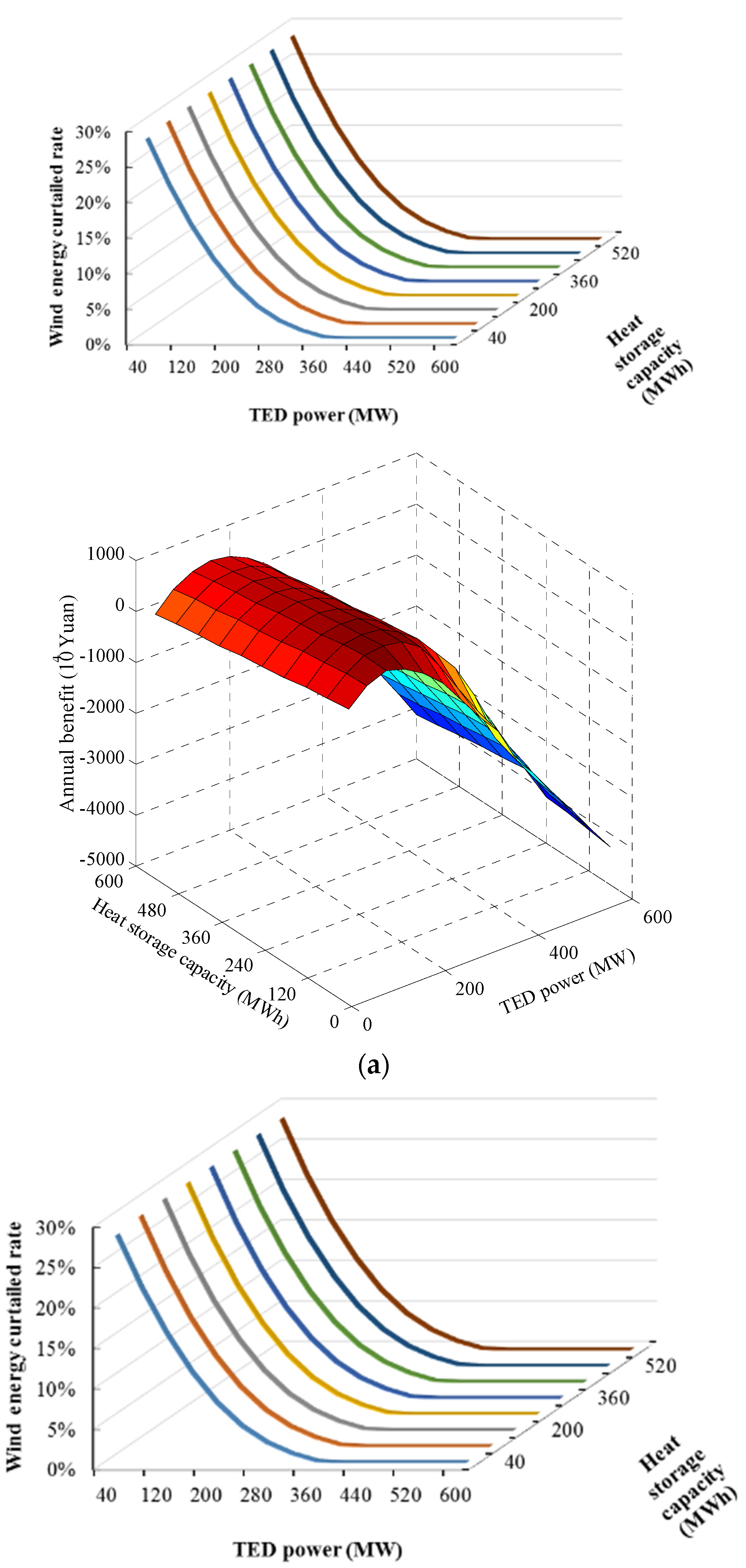
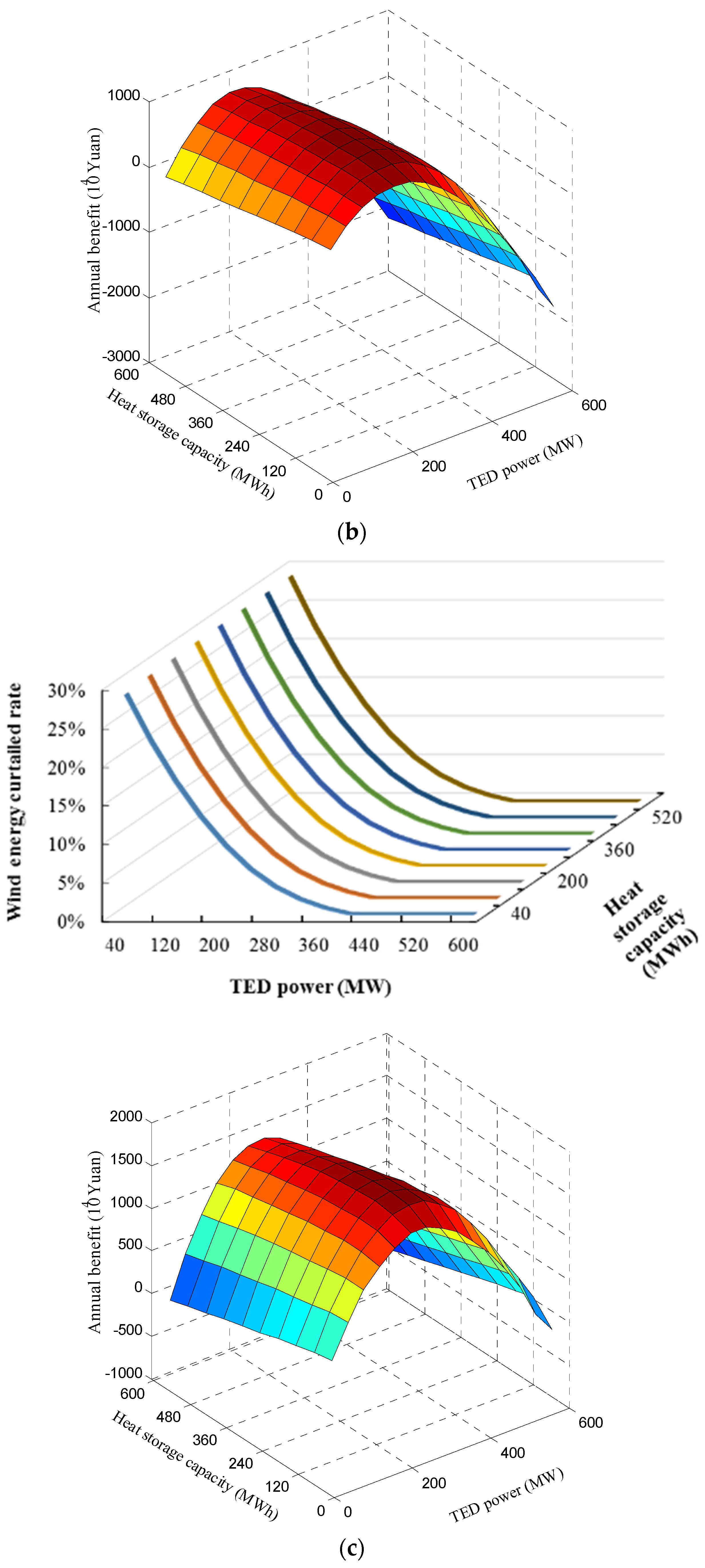
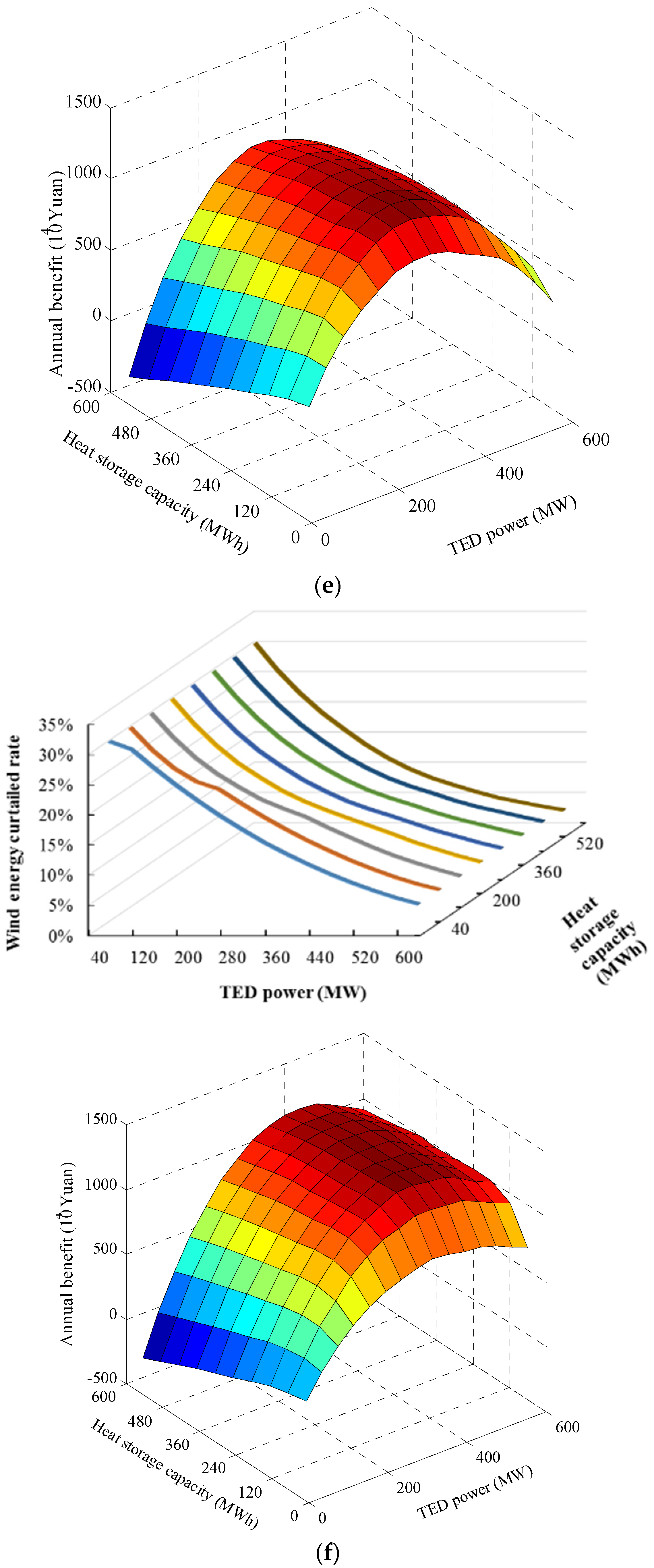
6.3. Simulation Results
| Scenario | The Ratio of between Psto and Pboile |
|---|---|
| A | 5:35 |
| B | 10:30 |
| C | 15:25 |
| D | 20:20 |
| E | 25:15 |
| F | 30:10 |
| G | 35:5 |

| Scenario | Computation Time (ms) | Speedup Ratio | |
|---|---|---|---|
| Serial Computing | Parallel Computing | ||
| A | 381.41 | 109.6 | 3.480018 |
| B | 401.72 | 443.28 | 0.906244 |
| C | 354.13 | 376.47 | 0.940659 |
| D | 421.65 | 113.46 | 3.716288 |
| E | 413.79 | 112.13 | 3.69027 |
| F | 388.58 | 109.78 | 3.539625 |
| G | 417.36 | 113.04 | 3.692144 |
| Total | 2778.64 | 1377.76 | 2.016781 |


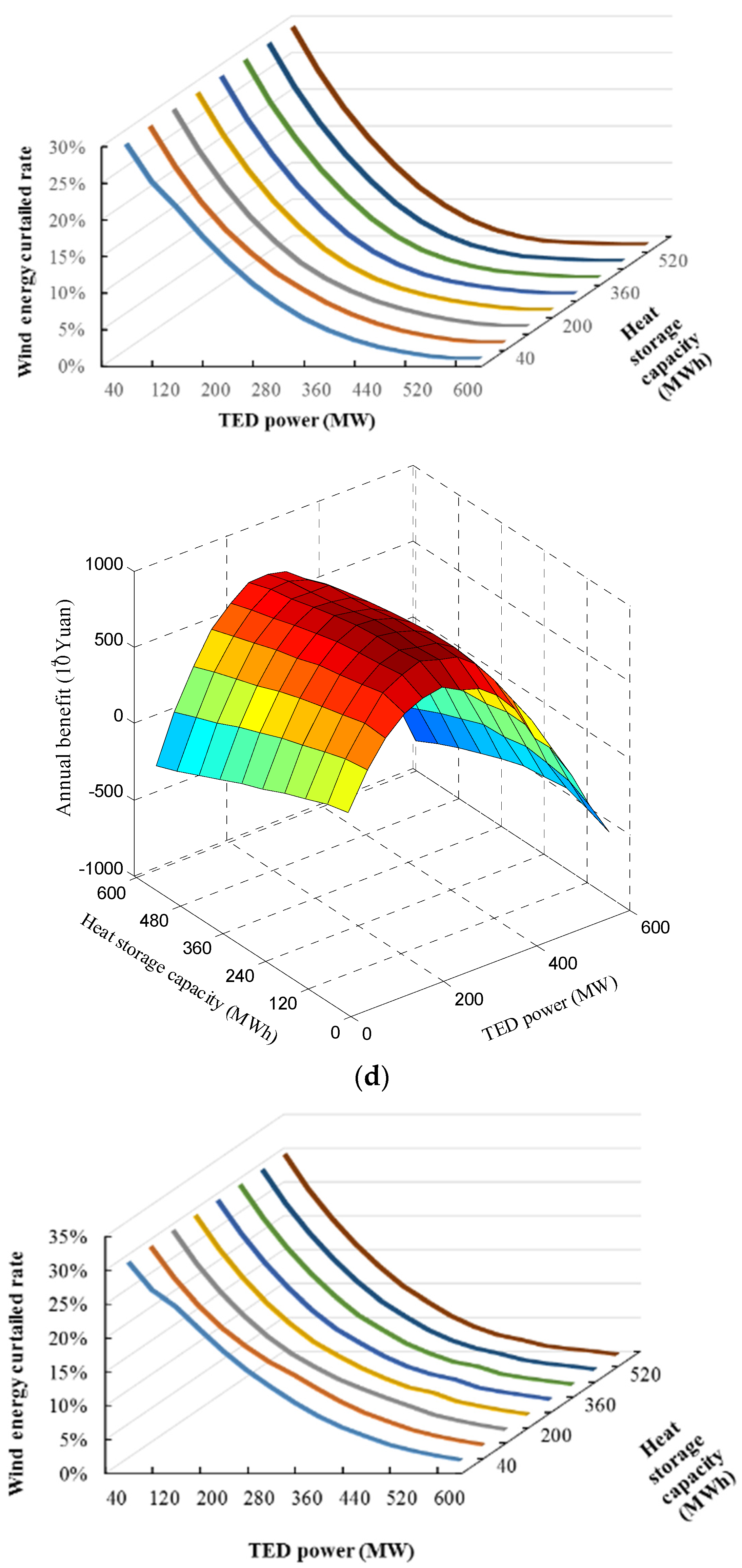


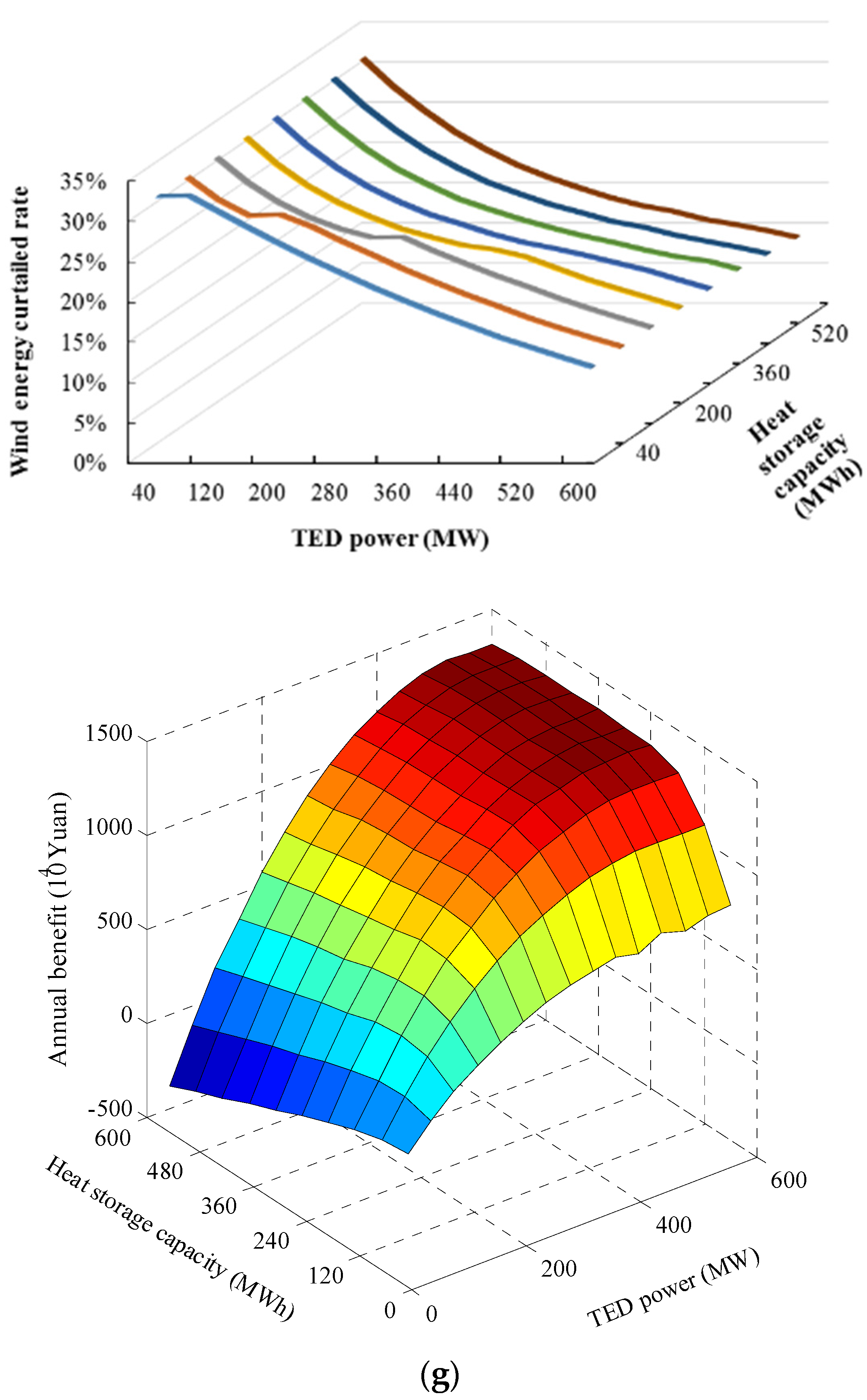
| Scenario | TED Power (MW) | Heat Storage Capacity (MWh) | Maximum Annual Profit (104 Yuan) | Wind Power Curtailment Rate | Wind Power Consumption by TED (GWh) |
|---|---|---|---|---|---|
| A | 160 | 115 | 967.5298 | 11.2% | 38.87617 |
| B | 245 | 180 | 985.908 | 5.7% | 48.48795 |
| C | 280 | 185 | 1690.164 | 6.8% | 46.51416 |
| D | 240 | 120 | 881.7941 | 12.2% | 37.14052 |
| E | 320 | 175 | 1089.603 | 13.9% | 34.08095 |
| F | 400 | 240 | 1211.144 | 17.0% | 28.71823 |
| G | 525 | 415 | 1339.6209 | 22.1% | 19.79877 |
7. Conclusions
Acknowledgments
Author Contributions
Conflicts of Interest
Nomenclature
| CHP | combine heat and power |
| TED | thermal-electric decoupling |
| annual incomes of TED | |
| annual fuel savings by lower electric power output | |
| annual fuel saving by less heat supply | |
| annual policy incomes | |
| cost of attached facilities | |
| annual cost of TED | |
| investment on electric boilers | |
| annual electric energy cost on system electric capacity tariff | |
| annual productive labor cost | |
| system installation and commissioning cost | |
| annual system maintaining and service cost | |
| heating to electric power output ratio of CHP unit n under backpressure condition | |
| annual operation cost | |
| cost of heat storage | |
| investment on electric transformation equipment | |
| initial investment of TED | |
| annual investment cost discount to present equivalent annual worth | |
| construction cost of workshops | |
| bank discount rate | |
| consumed wind energy by TED during the heating season | |
| storage capacity of heat storage within TED | |
| heating power output of heating boiler unit z at moment t | |
| heating power output of CHP unit n | |
| heating power output of TED unit k at moment t | |
| input heating power of TED unit k at moment t | |
| lower bounds of heating power output of heat source n | |
| lower bounds of heating power output of heat source n | |
| upper bond of heating power ramp rate of CHP unit n | |
| lower bonds of heating power ramp rate of CHP unit n | |
| maximum heat load during heating season | |
| a constant | |
| system electric load and power transfer to outside at cross-section | |
| system heating load | |
| number of wind turbines within wind farm | |
| annual benefit by installation of TED | |
| maximum power output by “Ordering Power by Heat” | |
| minimum electric power output by “Ordering Power by Heat” | |
| maximum electric power output of a CHP unit | |
| minimum electric power output of a CHP unit | |
| electric power output of non-CHP unit m at moment t | |
| electric power output of CHP unit n | |
| electric power output of wind turbine j at moment t | |
| input electric power of TED unit k at moment t | |
| upper bound of active power output of electric power generation unit n | |
| lower bound of active power output of electric power generation unit n | |
| upper bond of electric power ramp rate of CHP unit n | |
| lower bond of electric power ramp rate of CHP unit n | |
| consumed wind power by grid at moment t | |
| electric power input of TED unit k at moment t | |
| owned fund rate | |
| volume of heat storage | |
| fuel consumption rate of electricity generation of CHP n | |
| heat storage price per unit volume | |
| fuel consumption rate of heat generation of CHP n | |
| per unit policy income by emission reduction | |
| electric capacity tariff price per unit power per month | |
| construction cost of workshop per square meter | |
| scale parameter of Weibull’s distribution | |
| specific heat capacity of heat storage medium | |
| gravitation constant | |
| initial searching direction of algorithm calculating procedure | |
| new searching direction after meeting a saddle point | |
| maximum heating power output of a CHP unit | |
| forced minimum heat power output of a CHP unit by “Ordering Power by Heat” | |
| shape parameter of Weibull’s distribution | |
| wind speed | |
| cut-in wind speed | |
| cut-out wind speed | |
| rated wind speed | |
| an arbitrary initial value of algorithm calculating procedure | |
| new searching start value after meeting a saddle point | |
| position of a saddle point | |
| decreased heat power output of CHP n | |
| reduced electric power output of CHP n by TED at moment t | |
| temperature difference of heat storage medium | |
| path of integration for annual fuel saving | |
| emission quantity per unit mass fuel burning | |
| wake effect coefficient of wind farm | |
| Δ | variation factor of system load |
| corresponding eigenvectors of Jacobian matrix | |
| required precision of algorithm calculating procedure | |
| hourly system load (p.u.) | |
| daily heat load (p.u.) during heating season | |
| eigenvalues of Jacobian matrix | |
| density of heat storage medium | |
| weekly system electric load (p.u.) during heating season |
References
- Yang, X.; Song, Y.H.; Wang, G.H. Comprehensive Review on the Development of Sustainable Energy Strategy and Implementation in China. IEEE Trans. Sustain. Energy 2010, 22, 57–65. [Google Scholar] [CrossRef]
- Liang, R.H.; Liao, J.A. Fuzzy-Optimization Approach for Generation Scheduling with Wind and Solar Energy Systems. IEEE Trans. Power Syst. 2007, 4, 1665–1674. [Google Scholar] [CrossRef]
- Zhang, X.H.; Zhao, J.Q.; Chen, X.Y. Multi-objective Unit Commitment Fuzzy Modeling and Optimization for Energy-saving and Emission Reduction. Proc. CSEE 2010, 22, 71–76. [Google Scholar]
- The Renewable Energy Law of China. Available online: http://www.gov.cn/fwxx/bw/gjdljgwyh/content_2263069.htm (accessed on 15 October 2015).
- Global Wind Energy Council. Global Wind Report. Available online: http://www.gwec.net/publications/global-wind-report-2/global-wind-report-2014-annual-market-update/ (accessed on 15 October 2015).
- Wang, Z.Y.; Shi, J.L.; Zhao, Y.Q. The Roadmap of China Wind Power Development 2050, 1st ed.; Energy Research Institute, National Development and Reform Commission: Beijing, China, 2011; pp. 32–36. [Google Scholar]
- Wang, X.H.; Qiao, Y.; Lu, Z.X.; Ding, L.; Shao, G.H.; Xu, X.W.; Hou, K.Y. A Novel Method to Assess Wind Energy Usage in the Heat-supplied Season. Proc. CSEE 2015, 9, 2112–2119. [Google Scholar]
- Ibrahim, H.; Ilinca, A.; Perron, J. Energy storage systems-characteristics and comparisons. Renew. Sustain. Energy Rev. 2008, 5, 1221–1250. [Google Scholar] [CrossRef]
- Ibrahim, H.; Ilinca, A.; Perron, J. Comparison and analysis of different energy storage techniques based on their performance index. In Proceedings of the Electrical Power Conference 2007, Montreal, QC, Canada, 25–26 October 2007; pp. 393–398.
- Nourai, A. Large-scale electricity storage technologies for energy management. In Proceedings of the Power Engineering Society Summer Meeting 2002, Chicago, IL, USA, 21–25 June 2002; pp. 310–315.
- Kondoh, J.; Ishii, I.; Yamaguchi, H.; Murata, A.; Otani, K.; Sakuta, K.; Higuchi, N.; Sekine, S. Electrical energy storage systems for energy networks. Energy Convers. Manag. 2000, 7, 1863–1874. [Google Scholar] [CrossRef]
- Elsobki, M.S. Implementation of an integrated resource planning strategy: An optimal based formulation for co-generation applications. In Proceedings of the 14th International Conference and Exhibition on Electricity Distribution: Part 1 Contribution, London, UK, 2–5 June 1997; pp. 5–10.
- Fu, L.; Jiang, Y. Optimal Operation of Backpressure Units for Space Heating. Proc. CSEE 2000, 3, 81–84. [Google Scholar]
- Huang, S.H.; Chen, B.K.; Chu, W.C. Optimal operation strategy for cogeneration power plants. In Proceedings of IEEE Industry Applications Conference, Seattle, WA, USA, 3–7 October 2004; pp. 2057–2062.
- Guo, T.; Henwood, M.I.; van Ooijen, M. An algorithm for combined heat and power economic dispatch. IEEE Trans. Power Syst. 1996, 4, 1778–1784. [Google Scholar] [CrossRef]
- Long, H.Y.; Ma, J.W.; Wu, K. Energy conservation dispatch of power grid with mass cogeneration and wind turbine. Electr. Power Autom. Equip. 2011, 11, 18–22. [Google Scholar]
- Jiang, X.L.; Lu, Q.Y.; Xie, G.N. A Preconditioned Parallel Method for Solving Saddle Point Problems. Appl. Math. Mech. Engl. 2014, 9, 1011–1019. [Google Scholar]
- Rong, S.; Li, Z.M.; Li, W.X. Investigation of the Promotion of Wind Power Consumption Using the Thermal-Electric Decoupling Techniques. Energies 2015, 8, 8613–8629. [Google Scholar] [CrossRef]
- Yang, M.; Li, Z.M.; Cao, D.Y. Parallel algorithm for solving large-scale dense linear system on CUDA. Comp. Engl. Appl. 2011, 32, 27–30. [Google Scholar]
- Yang, M.; Sun, C.; Li, Z.M.; Cao, D.Y. An improved sparse matrix-vector multiplication kernel for solving modified equation in large scale power flow calculation on CUDA. In Proceedings of the Power Electronics and Motion Control Conference (IPEMC), Harbin, China, 2–5 June 2012; pp. 2028–2031.
© 2015 by the authors; licensee MDPI, Basel, Switzerland. This article is an open access article distributed under the terms and conditions of the Creative Commons by Attribution (CC-BY) license (http://creativecommons.org/licenses/by/4.0/).
Share and Cite
Rong, S.; Li, W.; Li, Z.; Sun, Y.; Zheng, T. Optimal Allocation of Thermal-Electric Decoupling Systems Based on the National Economy by an Improved Conjugate Gradient Method. Energies 2016, 9, 17. https://doi.org/10.3390/en9010017
Rong S, Li W, Li Z, Sun Y, Zheng T. Optimal Allocation of Thermal-Electric Decoupling Systems Based on the National Economy by an Improved Conjugate Gradient Method. Energies. 2016; 9(1):17. https://doi.org/10.3390/en9010017
Chicago/Turabian StyleRong, Shuang, Weixing Li, Zhimin Li, Yong Sun, and Taiyi Zheng. 2016. "Optimal Allocation of Thermal-Electric Decoupling Systems Based on the National Economy by an Improved Conjugate Gradient Method" Energies 9, no. 1: 17. https://doi.org/10.3390/en9010017