Online Energy Management of City Cars with Multi-Objective Linear Parameter-Varying L₂-Gain Control

Abstract

This work aims at online regulating transient current out of the batteries of small-sized electric cars that transport people and goods around cities. In a city with heavy traffic, transient current dominates the energy economy and propulsion capability, which are in opposition to each other. In order to manage the trade-off between energy consumption per distance and propulsion capability in transience, the authors improve on previous work on multi-objective linear parameter-varying (LPV) L₂-gain control. The observer embedded into this multi-objective controller no longer assumes Kalman-filtering structure, and structural conservatism is thus removed. A full-spectrum set of experiments is performed. The results reveal that the feedback design significantly improves energy-motion management.

1. Introduction

This work is concerned with online energy management of small-sized electric cars that can carry people and goods around a city with heavy traffic without discharging pollutants or green-house gases. There are currently four types of energy management systems that can be employed in city cars: (a) management of active power sources; (b) assistance with passive energy storage; (c) restructuring of power converters; and (d) implementation of control rules for the energy economy, as discussed in the sequel.

Most power sources available to the car industry suffer energy high ratios, either to cost or to weight. For example, lithium-ion batteries, fuel cells [1], high-capacity ultracapacitors, and ultrahigh-speed flywheels are too costly, and lead-acid batteries are too heavy. Therefore, it has become important for the industry to manage batteries to reduce consumption of electric energy. For example, researchers and practitioners put much effort into online measuring the state-of-charge and/or state-of-health of a diversity of batteries, and then regulating current outputs to decrease energy consumption per distance, while increasing the lifespan of the batteries [2,3,4,5,6,7]. Besides, parallel connection of ultracapacitors with batteries can boost energy efficiency. For example, ultracapacitors installed between batteries and power converters can increase the energy harvested in braking phases from mechanical kinetics to electricity [8,9]. Since capacitors are passive elements, they can efficiently absorb the impulsive currents out of boost choppers; otherwise, impulsive currents input to batteries merely become heat being dissipated instead of electricity being stored. There is the possibility that supercapacitors could also be employed for fast charging of city cars [10]. Furthermore, ultracapacitors deliver initial overshoots of currents to start motors, and thus are indispensable to fuel cell-powered city cars [11,12]. However, most city cars are lightweight and possess low horsepower, thus the amount of energy conserved in braking phases is limited, and the initial torque is usually large enough to start the motor.

Restructuring power converters can lead to vital reduction of electricity-to-heat, which has been well investigated by researchers and practitioners in the field of power-electronics control. For example, some designed multiple bi-directional DC/DC power converters to “soften” switching of currents, and RCD snubbers that network diodes with resistors and capacitors to reduce energy consumption from high-frequency switching [13,14,15]. Some have embedded microcontrollers into power converters for optimal timing of switching to suppress electricity loss [16,17,18,19]. In types (a), (b) and (c), energy management is focused on batteries and power converters, in which additional components are needed for the fulfillment of efficient energy. However, in type (d), a set of dynamic rules is programmed into the controller, an already existing component, to boost energetic economy [20,21,22,23], with the advantage of no additional hardware. This paper discusses type (d).

A city car is usually used for transportation within a heavy-traffic city; therefore, its transient current plays the leading role in economy of propulsion energy and safety of accelerating out of a busy crossing. Controlling current overshoots, which simultaneously dull the motion, can reduce energy dissipation per distance. This paper develops a multi-objective control to manage the trade-off between energy economy and motion dexterousness.

During the modeling process, we found through lab experiments that linear time-invariant (LTI) parameterization of city-car dynamics is unable to capture overshoots and the times the currents out of batteries rise. However, a city car is for transportation inside traffic jams, so its transient current plays the key to energy economy and driving safety. To this, we develop linear parameter-varying (LPV) modeling and identification to remedy such a situation, following the previous works in [24,25,26,27,28,29,30]. Here, the tire speed is taken as the slow-time state variable and simultaneously the scheduling parameter. Then, guided by dynamic duality, the parametric identification leads to an LPV plant that is well capable of matching its computed responses with the measured speed and current in both transient and steady states. Therein, the nonlinear dynamics in nature is represented as a second-order LPV plant served for feedback control.

The identified LPV plant is then combined into performance requirements upon energy consumption and motion transience per distance, rather than per time, to form a generalized plant served for multi-objective LPV $L_2$-gain control design. It is worth noting that the system is always under tracking of throttle commands and disturbances of gravity, so the energy-motion regulation is not specified by the mixed $H_{\infty }$/$H_2$ objective [31,32,33,34], which, in the last decade, has been more popular than double $L_2$-gain objective. Here the double-objective LPV $L_2$-gain feedback design is improved from the previous game-theoretic control in [23], such that the embedded observer is free of structure conservatism to yield much more excellent performance on energy-motion regulation. Therein, a feasible set of Luenberger gains is allowed, which are formulated into differential linear matrix inequalities (LMIs) by a slack variable, rather than being assumed with the structure of Kalman-filtering. Moreover, a finite-element method to numerically solve the differential LMIs arising from general rate-bounded LPV control is developed. This finite-element method removes the assumption that the system matrices be affine-dependent on the time-varying parameter for gain scheduling, which is usually made in the polygon or other convex-hull methods [33,34]. For the time being, such a finite-element method is the most general and non-conservative solver for differential LMIs.

Even though the sophisticated LMIs algebra was widely applied for feedback design for single $L_2$-gain objectives or mixed $H_{\infty }$/$H_2$ objectives [31,32,33,34], we did not apply them to multi-objective $L_2$-gain control, for the following reasons. Virtually LMI-based control starts at bounded real-lemmas (BRL), and then arrives at convex formulations of all feasible but unstructured controllers through elimination of decision matrices, e.g., in [35,36], or addition of slack variables, e.g., in [37,38]. The main difficulty of extending these BRL-stemmed strategies into multiple $L_2$-gain objectives is that the set of feasible closed-loop Lyapunov matrices is unable to numerically track back to a common output-feedback that achieves all $L_2$-gain objectives. Even conservatively assuming an identical Lyapunov matrix for all objectives, this difficulty still exists, although there is no such difficulty in state feedback [39,40,41]. For the present, the game-theoretic feedback control in the paper provides a solution to this difficulty.

Here the multiple $L_2$-gain control is going on a Nash game, wherein the players consist of several talkers, a worker, a disturber, a negotiator and an observer. The talkers have different $L_2$-gain demands, negotiating with one another through an agent. In a real time fashion, the worker delivers the control action to minimize the control storage plus estimation storage, while the disturber exerts plant disturbances, sensing noises and reference commands to maximize the storage. These two players against each other will make a decision at the same Nash equilibrium for all of the talkers’ demands, rather than bringing conservatism with decisions. An observer with the maximum disturber in mind comes into play for assisting the worker in reconstructing internal status of dynamics to make optimal decisions.

Including this introduction section, this paper is organized into eight sections. Section 2 details the improved version of multi-objective LPV $L_2$-gain control and Section 3 provides the finite-element solution of differential LMIs therefrom. Section 4 presents the dynamic modeling and identification of city cars. Section 5 applies the multi-objective control to online manage the energy-motion of city cars. Section 6 demonstrates the procedure of implementing the energy-motion management. Section 7 starts pilot runs in full spectrum and discusses the results therefrom. Section 8 recapitulates the present work.

2. Multi-Objective Linear Parameter-Varying (LPV) L₂-Gain Control

For the following pattern of generalized plants:

$$\begin{array}{l}\dot{x}=A(\text{ρ})x+B_1(\text{ρ})w+B_2(\text{ρ})u\\ {\Vert z_i\Vert }^2={\text{α}}_i^{-1}(\text{ρ})x^T{Q}_i(\text{ρ})x+{\Vert u\Vert }^2,i=1,\cdots ,n\\ y=C(\text{ρ})x+D(\text{ρ})w\end{array}$$

(1)

the feedback controllers are to be designed from the Nash-game perspective to achieve multiple $L_2$-gain objectives:

$${{\displaystyle {\int }_0^T\Vert z_i(t)\Vert }}^2\text{d}t\le {\displaystyle {\int }_0^T{\Vert w(t)\Vert }^2\text{d}t,\forall T>0,\forall w\in L_2[0,T],i=1,\cdots ,n}$$

(2)

under zero initial conditions. The matrices $(B_1,D)$ are firstly chosen as orthogonal to each other, i.e., $D{B}_1^T=0$, for canonically quadratic regulation.

Therein the measured output y is sent into the to-be-designed feedback controller that real-time regulates the control action u for the multi-objective performance of Equation (2) with the metric of $L_2$-gains from the exogenous disturbance w to its counterparts $z_i$’s. The exogenous disturbance w can be stacked up by plant disturbances, sensor noises, reference commands, and uncertainty-induced disturbances. The performance variables $z_i$’s are assigned for quadratic regulation of the state vector x and the control vector u, an example of which is $z_i={\left[\begin{array}{cc}u& {\text{α}}_i^{-1/2}{Q}_i^{1/2}x\end{array}\right]}^{\text{T}}$. Therein the matrices Q_i’s are positive-definite, and the performance indexes αi’s are positive scalars that quantify the negotiation among those individual $L_2$-gain objectives. All system matrices $(A,B_1,B_2,Q_i\prime s,{\alpha }_i\prime s,C,D)$ can be dependent on a real-time parameter ρ that is online measurable as the gain-scheduled vector of the feedback control; denote the range of the p-dimensional time-variant parameter ρ by Ω, i.e., $\forall \text{ρ}\in \mathrm{\Omega }\subset {\Re }^p$. Let the region of its variation-rates be contained by a polygon $\mathrm{\Gamma }$, i.e., $\dot{\rho }\in \mathrm{\Gamma }\subset {\Re }^p$, of which the vertices are denoted by ${\partial }_0\mathrm{\Gamma }$.

Let us first consider full-state feedback. Define the ith Hamiltonian H_i by:

$$H_i(x,u,w,\text{ρ})={\dot{V}}_i+{\Vert z_i\Vert }^2-{\Vert w\Vert }^2$$

(3)

where $V_i(x,\text{ρ})$ is a positive-definite quadratic storage of the current state, i.e.,

$$V_i(x,\text{ρ})=x^T{X}_i(\text{ρ})x;\hspace{1em}{X}_i=X_i^T>0,\hspace{1em}\forall \text{ρ}\in \mathrm{\Omega },\hspace{1em}i=1,\cdots ,n$$

(4)

Explicitly, the ith Hamiltonian H_i is:

$$H_i(x,u,w,\text{ρ})=x^T\dot{\text{ρ}}\cdot \frac{\partial X_i}{\partial \text{ρ}}x+2x^T{X}_i(Ax+B_{1}w+B_{2}u)+{\text{α}}_i^{-1}{x}^T{Q}_{i}x+u^{T}u-w^{T}w$$

(5)

where $\dot{\text{ρ}}\cdot \frac{\partial X_i}{\partial \text{ρ}}$ is the shorthand of ${\displaystyle \sum _{j=1}^p{\text{ρ}}_j\frac{\partial X_i}{\partial {\text{ρ}}_j}}$. Similar notations will appear in the sequel.

By “completing the square”, the ith Hamiltonian in Equation (5) appears to be:

$$\begin{array}{l}{H}_i(x,u,w,\text{ρ})=x^T(\dot{\text{ρ}}\cdot \frac{\partial X}{\partial \text{ρ}}+A^T{X}_i+X_{i}A+{\text{α}}_i^{-1}{Q}_i-X_i{B}_2{B}_2^T{X}_i+X_i{B}_1{B}_1^T{X}_i)x\\ +{\Vert u+B_2^T{X}_{i}x\Vert }^2-{\Vert w-B_1^T{X}_{i}x\Vert }^2\end{array}$$

(6)

Therefore, the minimum control $u_i^{*}$ and the maximum disturbance $w_i^{*}$ of the ith Hamiltonian H_i are, respectively:

$$u_i^{*}=-B_2^T{X}_{i}x,w_i^{*}=B_1^T{X}_{i}x$$

(7)

Substitution of Equation (7) into Equation (5) yields:

$$H_i(x,u_i^{*},w_i^{*},\text{ρ})=x^T{P}_{i}x$$

(8)

$$P_i\equiv \dot{\text{ρ}}\cdot \frac{\partial X}{\partial \text{ρ}}+A^T{X}_i+X_{i}A+{\text{α}}_i^{-1}{Q}_i-X_i{B}_2{B}_2^T{X}_i+X_i{B}_1{B}_1^T{X}_i$$

(9)

If $P_i<0$ for $\forall \text{ρ}\in \mathrm{\Omega }$, then the closed-loop is asymptotically stable and, with the definition in Equation (3):

$${{\displaystyle {\int }_0^T\Vert z_i(t)\Vert }}^2\text{d}t<{\displaystyle {\int }_0^T{\Vert w(t)\Vert }^2\text{d}t+V_i(x(0))-V_i(x(T))<{{\displaystyle {\int }_0^T\Vert w(t)\Vert }}^2\text{d}t},\hspace{1em}\forall w,\hspace{1em}\forall T>0$$

(10)

when $u=u_i^{*}$. This is just the ith objective of Equation (2).

Equation (7) reveals that the Nash equilibrium will be achieved if all the Hamiltonians $H_i$’s share the same control storage, i.e., $X_i=X$, $i=1,\cdots ,n$. That is, the control and the disturbance:

$$u_i^{*}=-B_2^{T}Xx,w_i^{*}=B_1^{T}Xx$$

(11)

are the minimum control and the minimum disturbance, respectively, of all Hamiltonians simultaneously. Based on Equation (9), the multiple $L_2$-gain objectives are all achievable if the following differential Riccati inequalities are feasible for $X>0$:

$$\mathrm{\beta }\cdot \frac{\partial X}{\partial \text{ρ}}+A^{T}X+XA+{\text{α}}_i^{-1}{Q}_i-X{B}_2{B}_2^{T}X+X{B}_1{B}_1^{T}X<0,\forall \mathrm{\beta }\in {\partial }_0\mathrm{\Gamma },i=1,\cdots ,n$$

(12)

Now let us continue to the output feedback embedded with a calibrated Luenberger observer:

$$\dot{\widehat{x}}=(A+W_{\text{cal}})\widehat{x}+B_{2}u+L(y-C_2\widehat{x})$$

(13)

where L is the Luenberger gain and W_cal is the calibration following the maximum disturbance $w^{*}$ in Equation (11) and the plant in Equation (1), that is:

$$W_{\text{cal}}=B_1{B}_1^{T}X$$

(14)

Define the error state by $\tilde{x}\equiv x-\widehat{x}$. Subtracting Equation (1) from Equation (13) in conjunction with Equation (14) yields:

$$\dot{\tilde{x}}=(A+B_1{B}_1^{T}X-LC)\tilde{x}+(B_1-LD)w-B_1{B}_1^{T}Xx$$

(15)

wherein all feasible Luenberger gains L are to be determined.

Inferred from the state-feedback above, the ith Hamiltonian function H_i assigned to the ith $L_2$-gain objective for the output feedback is to be:

$$H_i(x,\tilde{x},u,w,\text{ρ})=\frac{\text{d}V(x,\widehat{x},\text{ρ})}{\text{d}t}+{\Vert z_i\Vert }^2-{\Vert w\Vert }^2$$

(16)

where the ith storage function $V_i$ is chosen as control storage plus estimation storage, i.e.,

$$V_i(x,\tilde{x},\text{ρ})=x^{T}X(\text{ρ})x+{\tilde{x}}^T{Z}_i(\text{ρ})\tilde{x},X=X^T>0,Z_i=Z_i^T>0$$

(17)

With Equations (1) and (15), the ith Hamiltonian function H_i becomes:

$$\begin{array}{l}{H}_i(x,\tilde{x},u,w,\text{ρ})=x^T\dot{\text{ρ}}\cdot \frac{\partial X}{\partial \text{ρ}}x+{\tilde{x}}^T\dot{\text{ρ}}\cdot \frac{\partial Z_i}{\partial \text{ρ}}\tilde{x}\\ +2x^{T}X(Ax+B_{1}w+B_{2}u)+{\alpha }_i^{-1}{x}^T{Q}_{i}x+u^{T}u-w^{T}w\\ +2{\tilde{x}}^T{Z}_i[(A+B_1{B}_1^{T}X-LC)\tilde{x}+(B_1-LD)w-B_1{B}_1^{T}Xx]\end{array}$$

(18)

in which:

$$\frac{{\partial }^2{H}_i}{\partial w\partial u}=0$$

(19)

Known from the differential geometry, the minimum control $u_i^{*}$ and the maximum disturbance $w_i^{*}$ of the ith Hamiltonian H_i can be obtained through:

$$\frac{\partial H_i}{\partial u}(u=u_1^{*})=0,\frac{{\partial }^2{H}_i}{{\partial }^{2}u}(u=u_1^{*})>0$$

(20)

$$\frac{\partial H_i}{\partial w}(w=w_i^{*})=0,\frac{{\partial }^2{H}_i}{{\partial }^{2}w}(w=w_i^{*})<0$$

(21)

With Equations (19)–(21), it turns out that:

$$w_i^{*}=B_1^{T}Xx+{(B_1-LD)}^T{Z}_i\tilde{x},u_i^{*}=-B_2^{T}Xx$$

(22)

If we let $Z_i=Z$ for $\forall i$, Nash equilibrium is achieved when all Hamiltonians share the same control storage and estimation storage. Thus, in this multi-objective Hamiltonian game, the maximum disturbance is:

$$w^{*}=B_1^{T}Xx+{(B_1-LD)}^{T}Z\tilde{x}$$

(23)

However, the unavailability of the full information prevents the control u from being chosen as the minimum control, $u^{*}=-B_2^{T}Xx$. Instead, we choose:

$$u^{*}=-B_2^{T}X\widehat{x}$$

(24)

as the best estimation of the minimum control. Therein the temporal trajectory of maximum disturbance $w_i^{*}$ is evaluated by the maximum state-feedback in Equation (23), which is unable to destabilize the system. On ground of the principle of Equivalent Value in optimal control, the optimal decision to an open loop is identical at any time to the control input in optimal feedback, provided that the open-loop is asymptotically stable. Here the minimum feedback of Equation (24) stabilized the closed-loop system.

Substituting Equations (23) and (24) into Equation (18) yields:

$$H_i(x,\tilde{x},u^{*},w^{*},\rho )=x^T{P}_{i}x+{\tilde{x}}^Tℇ\tilde{x},i=1,\cdots ,n$$

(25)

$$P_i\equiv \dot{\rho }\cdot \frac{\partial X}{\partial \rho }+A^{T}X+XA+{\alpha }_i^{-1}{Q}_i-X{B}_2{B}_2^{T}X+X{B}_1{B}_1^{T}X$$

(26)

$$\begin{array}{l}ℇ\equiv \dot{\rho }\cdot \frac{\partial Z}{\partial \rho }+Z(A+B_1{B}_1^{T}X-LC)+{(A+B_1{B}_1^{T}X-LC)}^{T}Z\\ +X{B}_2{B}_2^{T}X+Z{B}_1{B}_1^{T}Z+ZLD{D}^T{L}^{T}Z\end{array}$$

(27)

If:

$$P_i<0,ℇ<0;X=X^T>0,Z=Z^T>0$$

(28)

then $H_i(x,\tilde{x},u^{*},w,\rho )<0$ for all w, $i=1,\cdots ,n$ will lead to the multi-objective $L_2$-gains performance specified in Equation (2).

Furthermore, setting $Y=ZL$ can rephrase Equation (27) to be:

$$ℇ\equiv \dot{\rho }\cdot \frac{\partial Z}{\partial \rho }+Z(A+B_1{B}_1^{T}X)+{(A+B_1{B}_1^{T}X)}^{T}Z-2YC+X{B}_2{B}_2^{T}X+Z{B}_1{B}_1^{T}Z+YD{D}^T{Y}^T$$

(29)

In summary, the multi-objective $L_2$-gain performance is achievable if the following LMIs-like inequalities are feasible for $X^{-1}>0$ and $Z>0$, for $\forall \omega \in \mathrm{\Omega }$:

$$\left[\begin{array}{ccc}-{\displaystyle \sum _{j=1}^p{\mathrm{\beta }}_j\frac{\partial X^{-1}}{\partial {\text{ρ}}_j}}+X^{-1}{A}^T+A{X}^{-1}-B_2{B}_2^T& X^{-1}{Q}_i^{1/2}& B_1\\ Q_i^{1/2}{X}^{-1}& -{\text{α}}_i& 0\\ B_1^T& 0& -I\end{array}\right]<0,\forall \mathrm{\beta }\in {\partial }_0\mathrm{\Gamma },i=1,\cdots ,n$$

(30)

$$\left[\begin{array}{cccc}+{\displaystyle \sum _{j=1}^p{\mathrm{\beta }}_j\frac{\partial Z}{\partial {\text{ρ}}_j}}+(Z{A}_{\text{cal}}+A_{\text{cal}}^{T}Z)-(YC+C^T{Y}^T)& YD& Z{B}_1& X{B}_2\\ D^T{Y}^T& -I& 0& 0\\ B_1^{T}Z& 0& -I& 0\\ B_2^{T}X& 0& 0& -I\end{array}\right]<0,\forall \mathrm{\beta }\in {\partial }_0\mathrm{\Gamma }$$

(31)

where $A_{\text{cal}}=A+B_1{B}_1^{T}X$ and $Y$ is a slack variable. Any quadruple $(X,Z,Y,{\text{α}}_i)$ satisfying Equations (30) and (31) defines a feasible feedback. The Luenberger gain is then calculated by $L=Z^{-1}Y$, and the feedback controllers take the form:

$$\begin{array}{l}\dot{\widehat{x}}=(A+B_1{B}_1^{T}X-B_2{B}_2^{T}X-LC)\widehat{x}+Ly\\ u=-B_2^{T}X\widehat{x}\end{array}$$

(32)

Extended from the canonical LQ optimal control, this game-theoretic strategy provides a solution to multi-objective $L_2$-gain robust control without bringing conservatism into the feasibility.

3. Finite-Element Solution of the Differential Linear Matrix Inequalities (LMIs)

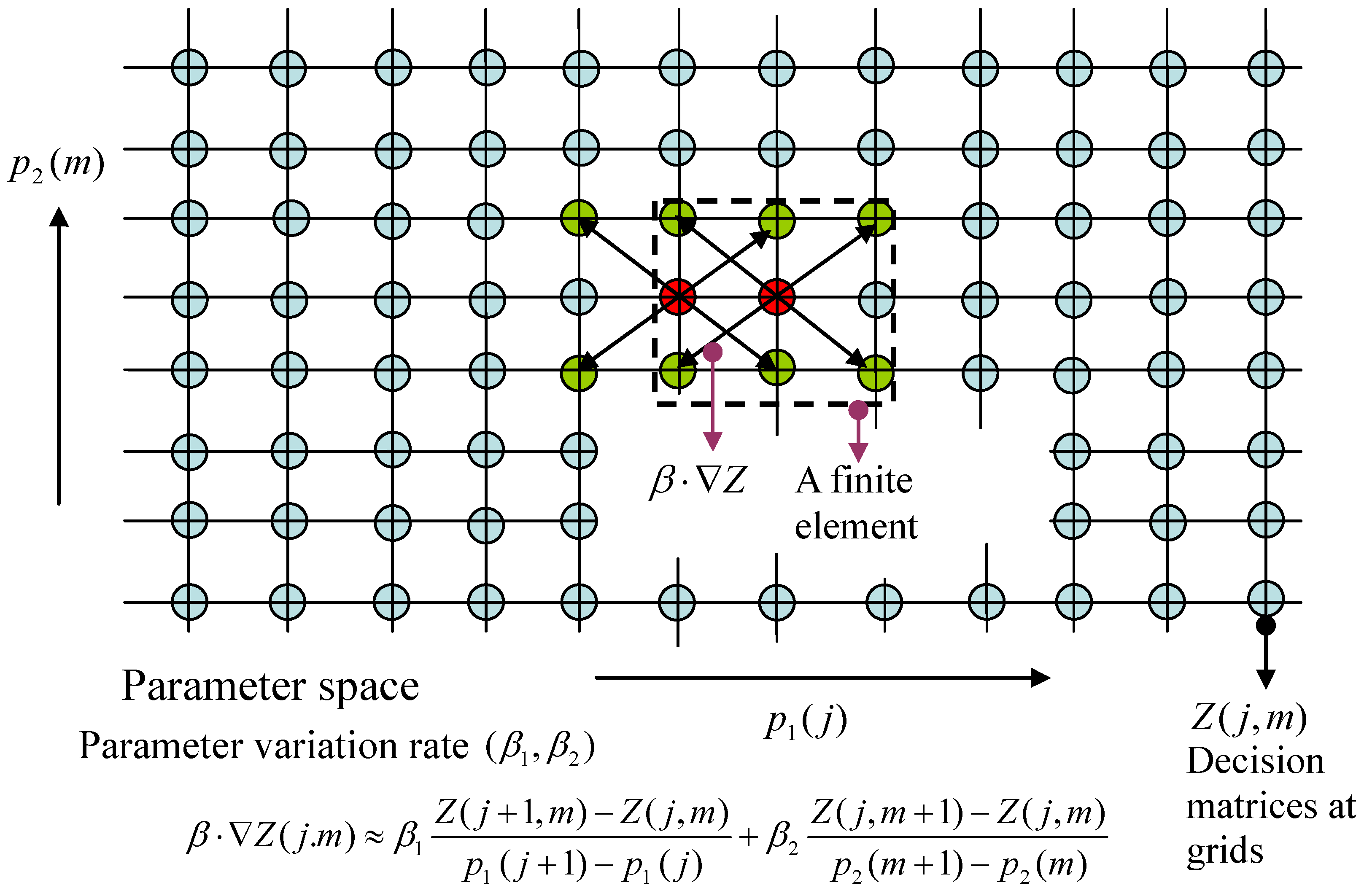
Partition the parameter space Ω into N elements $\left\{\Delta (k):k=1,\cdots ,N\right\}$ centered at the grid points: $\left\{\rho (k):k=1,\cdots ,N\right\}$. Denote the gradient of the function Z by $\nabla Z$, wherein the ith component of $\nabla Z$ is $\partial Z/\partial {\rho }_i$ for $i=1,\cdots ,p$. Moreover, the gradient of Z at the kth grid $\text{ρ}(k)$ is denoted by $\nabla Z(k)$. The same notation is also used for the decision function $X^{-1}$. The gradient $\nabla Z(k)$ involves not only the point $\text{ω}(k)$ but also the grid points at its neighborhood.

In the following an explanatory example for $p=2$, referring to Figure 1, is provided. Let the 2D Cartesian plane be coordinated by components of the parameter, $p_1$ and $p_2$, wherein the $p_1$-axis and $p_2$-axis are discretized by $\left\{p_1(1),p_1(2),\cdots \right\}$ and $\left\{p_2(1),p_2(2),\cdots \right\}$, respectively. Put the parameter space $\mathrm{\Gamma }$ into this 2D grid, and find all nodes $(p_1(j),p2(m))$, $\forall j\in J$, $\forall m\in M$, inside Ω. As such, Ω is the union of a number of finite elements centered at:

$$\left\{(p_1(j),p_2(m)):j\in j,m\in M\right\}$$

(33)

at which the values of the decision functions are to be solved. If the value of the decision function $Z$ at the point $(p_1(j),p_2(m))$ is notated by $Z(j,m)$, then the inner-product $\mathrm{\beta }\cdot \nabla Z$ at that point can be approximated by:

$$\mathrm{\beta }\cdot \nabla Z(j.m)\approx {\mathrm{\beta }}_1\frac{Z(j+1,m)-Z(j,m)}{p_1(j+1)-p_1(j)}+{\mathrm{\beta }}_2\frac{Z(j,m+1)-Z(j,m)}{p_2(m+1)-p_2(m)}$$

(34)

Similar notations become clear for $p>2$.

Figure 1. Finite-element approximation of differential linear matrix inequalities (LMIs).

Figure 1. Finite-element approximation of differential linear matrix inequalities (LMIs).

For brevity of notations, let the differential LMIs of Equations (30) and (31) be written, respectively, by:

$$L_X(\mathrm{\beta }\cdot \nabla X^{-1},X^{-1},\text{ρ},i)<0,\forall \text{ρ}\in \text{Ω},\forall \mathrm{\beta }\in {\partial }_0\mathrm{\Gamma },\forall i=1,\cdots ,n$$

(35)

$$L_Z(\mathrm{\beta }\cdot \nabla Z,Z,\text{ρ})<0,\forall \text{ρ}\in \mathrm{\Omega },\forall \mathrm{\beta }\in {\partial }_0\mathrm{\Gamma }$$

(36)

With the above notations, the finite-element version of the differential LMIs of Equations (30) and (31) become, respectively:

$$L_X(\mathrm{\beta }\cdot \nabla X^{-1}(k),X^{-1}(k),\text{ρ}(k),i)<0,\forall \mathrm{\beta }\in {\partial }_0\mathrm{\Gamma },k=1.\cdots ,N,i=1,\cdots ,n$$

(37)

$$L_Z(\mathrm{\beta }\cdot \nabla Z(k),Z(k),\text{ρ}(k))<0,\forall \mathrm{\beta }\in {\partial }_0\mathrm{\Gamma },\forall k=1,\cdots ,N$$

(38)

which spawn $qNn$ and $qN$ LMIs, respectively, where $q$ is the number of vertices of the polygon $\mathrm{\Gamma }$ that bounds the parameter variation-rates.

For a feasible set of $L_2$-gain indexes ${\alpha }_i$’s, firstly call ‘feasp’ in the Matlab-LMI toolbox to solve the feasible solution of Equation (37), which outputs the minimum solution $X_{\min }$ over $\text{ρ}\in \mathrm{\Omega }$, that is X_min − X < 0, $\text{ρ}\in \mathrm{\Omega }$, $\forall \text{ρ}\in \mathrm{\Omega }$. Secondly, substitute the solution $X_{\min }$ into Equation (38), and then call the ‘mincx’ routine to obtain, if feasible, the solution $Z_{\max }$ with minimum integration of trace over $\text{ρ}\in \mathrm{\Omega }$: ${\displaystyle \sum _{k=1}^{N}trZ(k)\Delta (k)}$, which maximizes the Luenberger gain $L$. This strategy is named here “min-action-max-estimation”.

4. Modeling and Identification of Car Dynamics

The city car with speed under 55 km/h appears as the one in Figure 2.

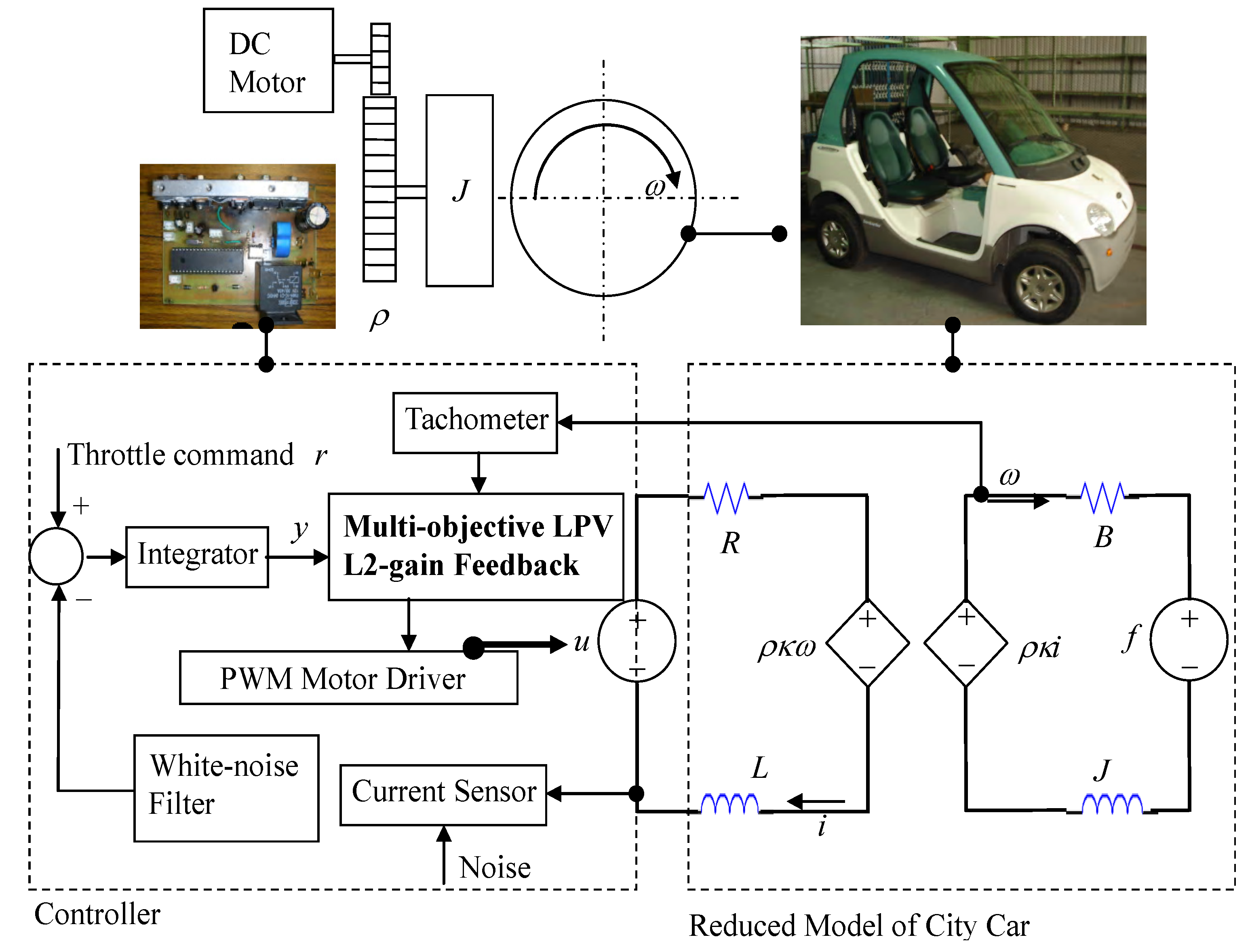
Figure 2. Modeling and controller design of DC-motorized city cars.

Figure 2. Modeling and controller design of DC-motorized city cars.

Its dynamics served for modeling, identification and feedback design is reduced with the following aspects of simplification:

(A1)

There is no slippage in the gear transmission.

(A2)

The rotor in the DC-motor has negligible inertia of rotation.

(A3)

In the motor, the coefficient of counter electromagnetic force is equal to the torque coefficient.

(A4)

For the motor, the allowed current, speed, and power are invariant to changes of the load.

(A5)

The tires roll on the road nearly always without slipping.

(A6)

The mass centers of tires are coincident with the centers of bearing.

(A7)

The wind resistance is nearly linearly dependent on car speed.

(A8)

Consider the city car moving along a straight line.

With (A1)–(A8) and electromechanical principles, the city-car dynamics in Figure 2 can be parameterized to second order with electric inductance L, electric resistance R, equivalent inertia of rotation J, mechanical damping B, gear ratio ρ, and torque coefficient $\kappa$. The input includes the controlled voltage u, being the electric effort across the motor, and the equivalent torque f, being the mechanical effort from the gravity of uphill. The state of dynamics consists of the motor current i, being the fast-time state variable, and the tire speed ω, being the slow-time state. With (A5), Lagrange dynamics formulates the equivalent inertia J and the equivalent torque f to be:

$$J=m{r}_t^2+4J_t;f=mg{r}_t\sin \text{φ}$$

(39)

where m stands for the total mass of the car plus its driver, $J_t$ for the rotation inertia of each tire at the wheel hub (assuming four tires to be identical), $r_t$ for the radius of each tire, and φ for the inclination angle of the road surface from the horizon.

Parametric identification is further performed in the sequel. Based on the postulation of dynamic duality, we found on experimental account the following rules:

(DD-1)

Like the mechanical inertia, the electric inertia is a constant.

(DD-2)

The electric resistance is monotonically increased with the tire speed, while the mechanical damping is monotonically decreased with the speed.

(DD-3)

The torque coefficient (counter electromagnetic coefficient) is a constant.

With (DD-1), the electric inductance $L$ is taken as a constant. Without the mechanical load, the response of motor current in the neighborhood of initial time is generated by the transfer function $1/(Ls+R_0)$, where $R_0$ is the static resistance. Give the motor a step voltage to measure the overshoot and time constant of rising current, which identify the electric inductance $L$ and the steady-state resistance $R_0$, respectively. Then, vary the step voltages to measure rotation speeds of the motor in steady state, and record the result. It shows a linear relationship between the motor voltage and the motor speed in steady state, when the steady-state current is close to zero. Therefore, the torque coefficient $\kappa$ is a constant, consistent with (DD-3).

With (DD-2), Kirchhoff’s theorems upon the equivalent circuit in Figure 2 realizes the state space of the car dynamics to be:

$$\begin{array}{l}L\frac{\text{d}i}{\text{d}t}=-R(\text{ω})\text{\hspace{0.05em}\hspace{0.05em}}i-\text{ρκω}+u\\ J\frac{\text{dω}}{\text{d}t}=\text{ρκ}i-B(\text{ω)ω}+f\end{array}$$

(40)

With this LPV parameterization, we are ready for identification of the speed-dependent electric resistance $R$ and the mechanical damping $B$. Let the car on the road be maneuvered by the driving of pulse-width modulated voltages $\overline{u}$ and the braking of road-surface inclinations $\overline{f}$, both of which are measured and recorded. 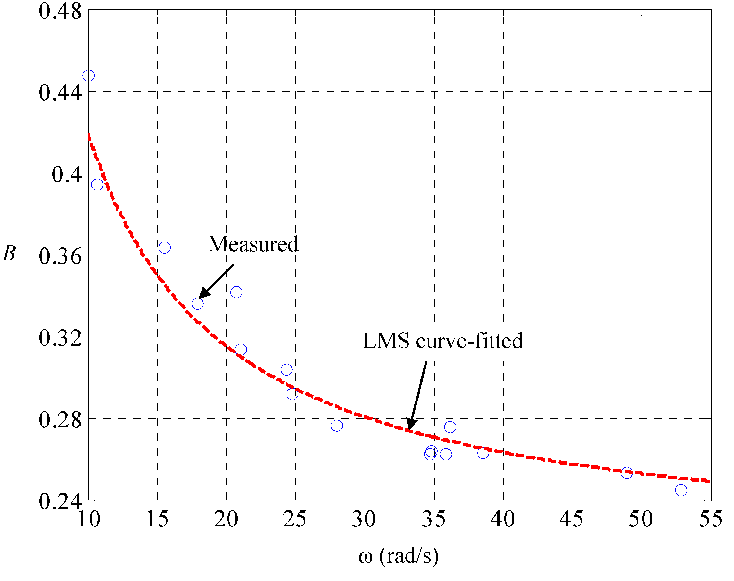A different $(\overline{u},\overline{f})$ makes a different $(\overline{i},\overline{\text{ω}})$, the current and speed in steady state, and there is one-to-one mapping between them. 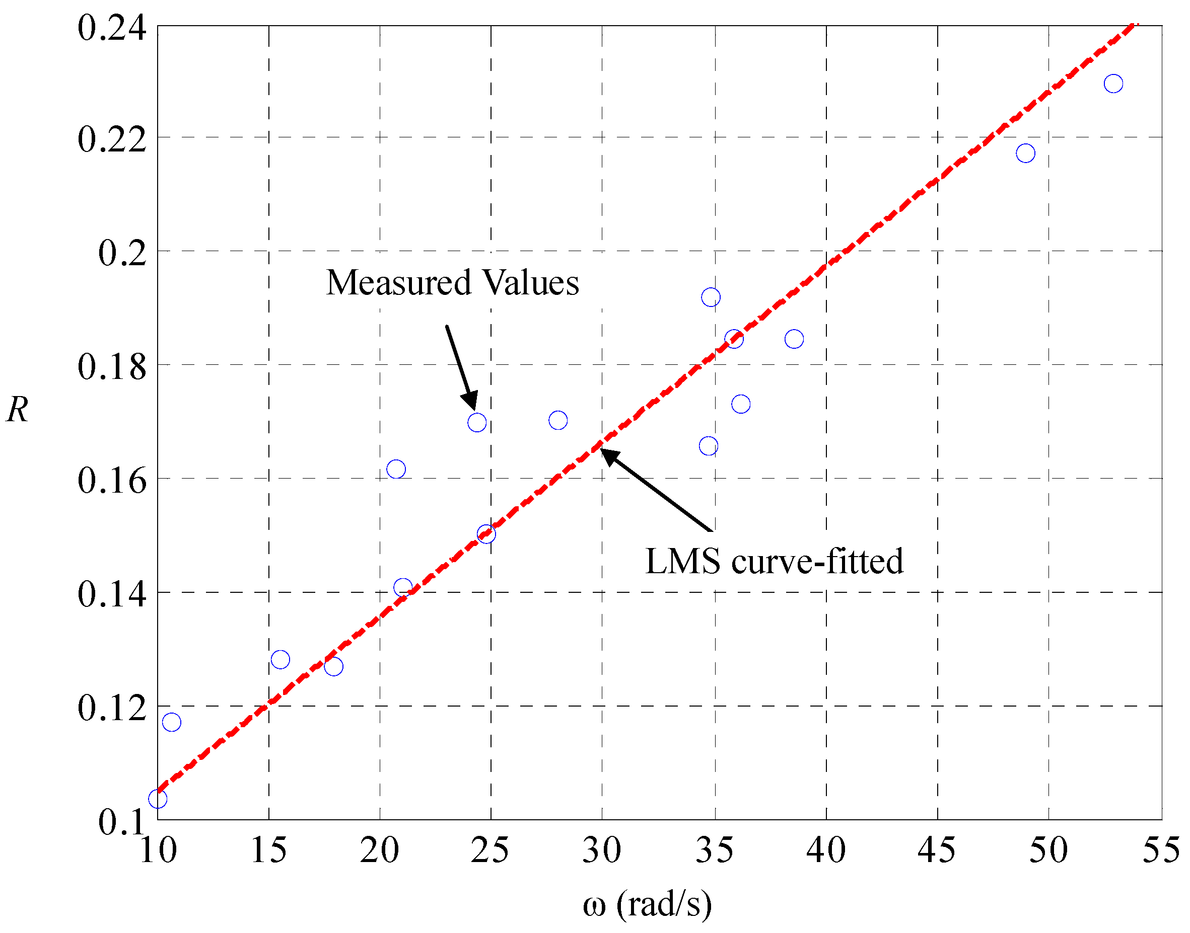The result is found to be in line with (DD-2), as shown in Figure 3 and Figure 4, respectively. Since the mechanical friction in low-speed region is close to the static friction, the mechanical damping ought to be nearly inversely proportional to the tire speed with an offset representing the dynamic damping in high-speed region. The tire speed represents the mechanical flow but the counter effort in the electric part, so that the electric resistance ought to be nearly linearly proportional to the speed, with an offset representing the static resistance.

Figure 3. Identification of dependence electric resistance on tire speed.

Figure 3. Identification of dependence electric resistance on tire speed.

Figure 4. Identification of dependence of mechanical damping on tire speed.

Figure 4. Identification of dependence of mechanical damping on tire speed.

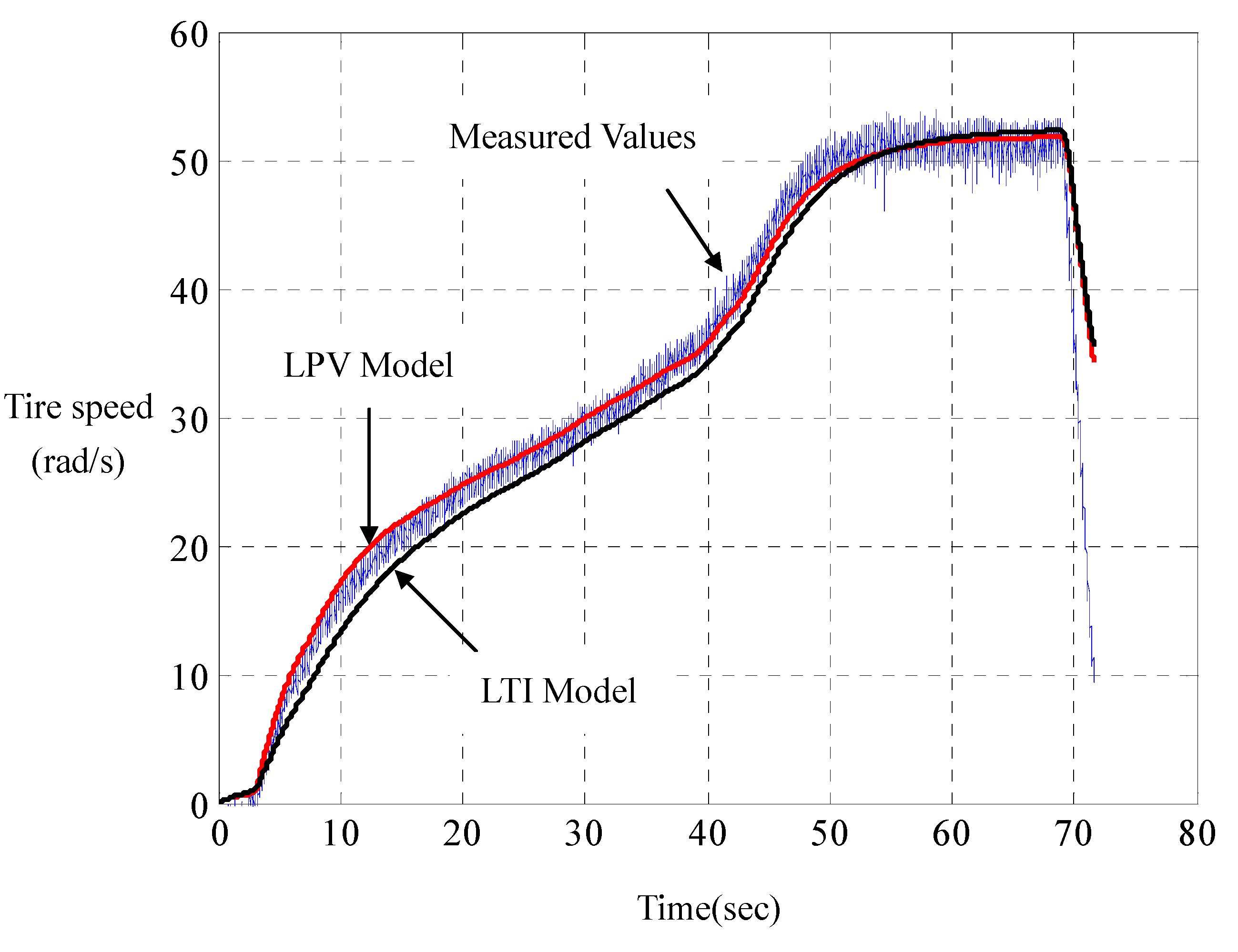
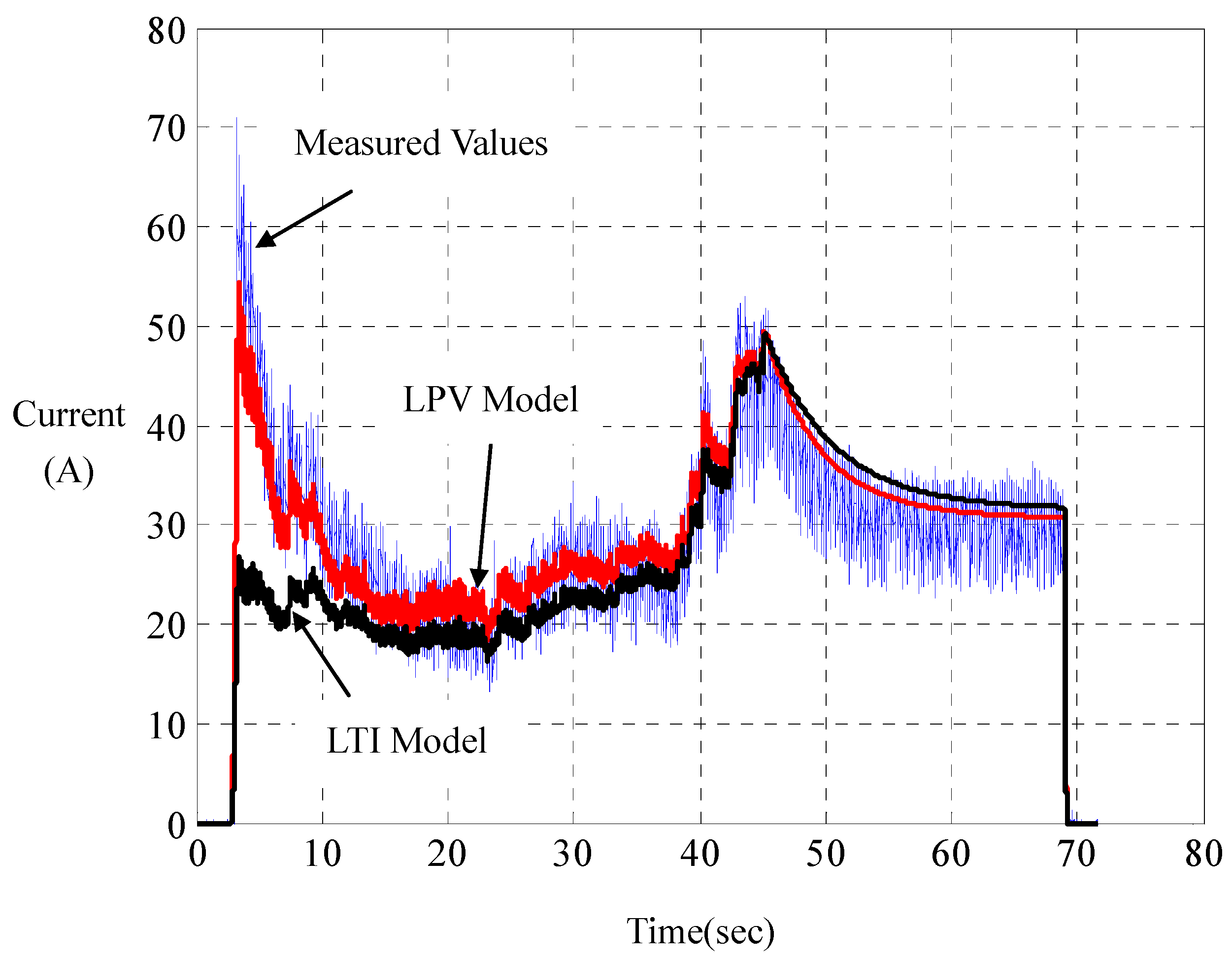
Experiments joining the computer simulations show that such LPV parameterization has its computed responses in perfect agreement with those measured on the road, whereof a represented result is shown in Figure 5 and Figure 6. For comparison, the responses of the linear LTI model with steady-state resistance $R_0$ and damping $B_0$ are also computed. Unlike LPV parameterization, LTI parameterization is unable to capture overshoots and rising times of the motor currents in practice. With road tests on a set of road-surface inclinations and driving-voltage curves, it is found that such a LPV modeling really catches the car dynamics. This indirectly verifies the principle of dynamic duality in LPV parameterization for city cars, as proposed in (DD-1), (DD-2) and (DD-3).

Figure 5. Current comparison of linear parameter-varying (LPV) with linear time-invariant (LTI) parameterizations.

Figure 5. Current comparison of linear parameter-varying (LPV) with linear time-invariant (LTI) parameterizations.

Figure 6. Speed comparison of LPV with LTI parameterizations.

Figure 6. Speed comparison of LPV with LTI parameterizations.

The state variables ω and i, the time t, the electric effort u, and the mechanical effort f in Equation (40) can be further made dimensionless by:

$$\text{ω}\to \frac{\text{ω}}{\overline{\text{ω}}},i\to \frac{i}{\overline{i}},t\to \frac{t}{{\text{τ}}_{\text{m}}},u\to \frac{u}{\overline{u}},f\to \frac{f}{B(1)\cdot \overline{\text{ω}}}$$

(41)

where $\overline{u}$ stands for the battery voltage (assuming that buck chopper is used), $\overline{\text{ω}}$ and $\overline{i}$ for the level speed and current, respectively, in steady state, as the motor voltage is kept at $\overline{u}$. The ${\text{τ}}_{\text{m}}$ stands for the time constant of mechanical parts $J/B(1)$. Moreover, dimensionless resistance λ and dimensionless damping b are defined, respectively, by:

$$\text{λ}(\text{ω})\equiv \frac{R(\text{ω})}{R(1)};b(\text{ω})\equiv \frac{B(\text{ω})}{B(1)}$$

(42)

The order-reduced dynamics is thus LPV-parameterized by:

$$\begin{array}{l}\frac{\text{d}i}{\text{d}t}=-\text{βλ(ω})i-\text{φω}+(\mathrm{\beta }+\text{φ})u\\ \frac{\text{dω}}{\text{d}t}=i-b(\text{ω})\text{ω}-f\end{array}$$

(43)

where β and φ indicate mechatronic ratios of AC characteristics and power ratings of electric vehicles, respectively. In the sequel, this identified LPV modeling is combined with energy and motion objectives to form a generalized plant, served for feedback design.

5. Energy-Motion Management

Referring to the left part of Figure 2, the following symbols are employed to construct a generalized plant. There are four state variables:

(i)

$x_1$: The motor current i related to the rate of energy dissipated from the electric resistor.

(ii)

$x_2$: The tire speed ω related to the rate of energy dissipated from the mechanical damper.

(iii)

$x_3$: The integration of tracking error of motor current $e_1=r-i$, which indicates the quickness of acceleration under servocontrol.

(iv)

$x_4$: The integration of tracking error of tire speed $e_2=r-\text{ω}$, which indicates the quickness of speed under servocontrol, where $r\in [0,1]$ is the reference command.

The former two state variables, x₁ and x₂, quantify the rate of energy consumption, and the latter two state variables, x₃ and x₄ indicate the responses of motion.

Also defined are the general disturbance and two performance counterparts as well as two performance indexes:

(v)

$q={\left[\begin{array}{ccc}r& f& \text{θ}\end{array}\right]}^T$: The general disturbance consisting of the command reference $r$, the inclined gravity $f$, and the measurement contamination θ that is the temporal integration of current-sensor noise after white-noise filtering, as shown in Figure 2.

(vi)

$z_1={\left[\begin{array}{ccc}{\gamma }_1^{-1}{x}_3& {\gamma }_1^{-1}{x}_4& u\end{array}\right]}^T$: The performance variable related to quickness-in-motion (QM).

(vii)

$z_2={\left[\begin{array}{ccc}{\gamma }_2^{-1}{x}_1& {\gamma }_2^{-1}{x}_2& u\end{array}\right]}^T$, The performance variable related to economy-in-energy (EE).

(viii)

${\text{γ}}_1>0$ is the performance index of QM, when the closed-loop $L_2$-gain from the general disturbance $q$ to the QM variable $z_1$ is set to one:

$${\displaystyle {\int }_0^T{\left|z_1(t)\right|}^2\text{ω}(t)}\text{d}t<{\displaystyle {\int }_0^T{\left|q(t)\right|}^2\text{ω}(t)}\text{d}t,\forall T\in [0,\infty )$$

(44)

where the $L_2$-norms of both sides are of integrations by distance $\text{d}s=\text{ω\hspace{0.17em}d}t$so that $L_2$-gain performance is signified by per-distance rather than by per-time.

(ix)

${\text{γ}}_2>0$ is the performance index of EE, when the closed-loop $L_2$ -gain from the general disturbance $q$ to the EE variable $z_2$ is also set to one:

$${\displaystyle {\int }_0^T{\left|z_2(t)\right|}^2}\text{ω}(t)\text{d}t<{\displaystyle {\int }_0^T{\left|q(t)\right|}^2}\text{ω}(t)\text{d}t,\forall T\in [0,\infty )$$

(45)

where the $L_2$-norms are weighted by the tire speed ω to emphasize energy consumption per distance.

A smaller QM-index γ1 implies that the distance for reaching the reference speed or torque is shorter, that is, the motion is quicker under servocontrol. A smaller EE-index γ₂ means that heat generation from mechanical damper and electric resistor is less in transience per distance. The QM-variable $z_1$ and EE-variable $z_2$ include the motor voltage u as an entry to protect both objectives from being achieved by cheap control, whereby to keep the motor voltage within a practical range in real operations.

As the $L_2$-gains of Equations (44) and (45) are per-distance specified, we replace the performance variables, the general disturbance, the motor voltage, and the output (the input to the controller as shown in Figure 2) by:

$${\widehat{z}}_1=\sqrt{\text{ω}}{z}_1,{\widehat{z}}_2=\sqrt{\text{ω}}{z}_2,\widehat{q}=\sqrt{\text{ω}}q,\widehat{u}=\sqrt{\text{ω}}u\hspace{1em}\text{and}\hspace{1em}\widehat{y}=\sqrt{\text{ω}}y$$

(46)

respectively, in order to construct the generalized plant served for the control design in Section 2. Combination of performance requirements in Equations (44) and (45) and the nominal plant in Equation (43) results in the following LPV generalized plant:

$$\left[\begin{array}{c}{\dot{x}}_1\\ {\dot{x}}_2\\ {\dot{x}}_3\\ {\dot{x}}_4\end{array}\right]=\left[\begin{array}{cccc}-\text{βλ}(\text{ω})& -\varphi & 0& 0\\ 1& -b(\text{ω})& 0& 0\\ -1& 0& -{\text{ε}}_1& 0\\ 0& -1& 0& -{\text{ε}}_2\end{array}\right]\left[\begin{array}{c}{x}_1\\ x_2\\ x_3\\ x_4\end{array}\right]+\frac{1}{\sqrt{\text{ω}}}\left[\begin{array}{ccc}0& 0& 0\\ 0& -1& 0\\ 1& 0& {\text{ε}}_3\\ 1& 0& 0\end{array}\right]\widehat{q}+\frac{1}{\sqrt{\text{ω}}}\left[\begin{array}{c}\text{β+}\varphi \\ 0\\ 0\\ 0\end{array}\right]\widehat{u}$$

(47)

$${\widehat{z}}_1={\text{γ}}_1^{-1}\sqrt{\text{ω}}\left[\begin{array}{cccc}0& 0& 1& 0\\ 0& 0& 0& 1\\ 0& 0& 0& 0\end{array}\right]\left[\begin{array}{c}{x}_1\\ x_2\\ x_3\\ x_4\end{array}\right]+\left[\begin{array}{c}0\\ 0\\ 1\end{array}\right]\widehat{u}$$

(48)

$${\widehat{z}}_2={\text{γ}}_2^{-1}\sqrt{\text{ω}}\left[\begin{array}{cccc}1& 0& 0& 0\\ 0& 1& 0& 0\\ 0& 0& 0& 0\end{array}\right]\left[\begin{array}{c}{x}_1\\ x_2\\ x_3\\ x_4\end{array}\right]+\left[\begin{array}{c}0\\ 0\\ 1\end{array}\right]\widehat{u}$$

(49)

$$\widehat{y}=\sqrt{\text{ω}}\left[\begin{array}{cccc}0& 0& 1& 0\end{array}\right]\left[\begin{array}{c}{x}_1\\ x_2\\ x_3\\ x_4\end{array}\right]+\left[\begin{array}{ccc}0& 0& 1\end{array}\right]\widehat{q},\text{ω}\in [\text{ε},1]$$

(50)

where small positive values ${\text{ε}}_1$ and ${\text{ε}}_2$, which indicate relaxed integrations, are chosen to replace zeros to avoid the singularity of $L_2$-gain control regarding to DC disturbances. Moreover, a freely chosen parameter ${\text{ε}}_3$ is also included for additional weighing on torque tracking.

Equations (47)–(50) can be briefly written as:

$$\begin{array}{l}\dot{x}=A(\text{ω})x+B_1(\text{ω})\widehat{q}+B_2(\text{ω})\widehat{u}\\ {\widehat{z}}_1={\text{γ}}_1^{-1}{C}_{11}(\text{ω})x+D_{12}\widehat{u}\\ {\widehat{z}}_2={\text{γ}}_2^{-1}{C}_{12}(\text{ω})x+D_{22}\widehat{u}\\ \widehat{y}=C_2(\text{ω})x+D_{21}\widehat{q}\end{array}$$

(51)

where the tire speed $\text{ω}\in [\text{ε},1]$ plays as the slow-time gain-scheduling parameter, other than a state variable, in LPV control. In case of $\text{ε}=0$, the state-space realization of Equation (51) will be uncontrollable and unobservable. In practice, the positive number ε can be set arbitrarily close to zero. The rate-bounds of the tire speed are assumed available at the stage of propulsion design:

$$\stackrel{⌣}{\mathrm{\beta }}\le \dot{\text{ω}}\le \stackrel{⌣}{\mathrm{\beta }}$$

(52)

The LPV generalized plant of Equation (51) is served for multi-objective LPV $L_2$-gain control design presented in Section 2.

The feedback design in Section 2 in conjunction with its finite-element solver in Section 3 is then employed to solve feasible quadruples $(X,Z,{\text{γ}}_{\text{1}}{\text{,γ}}_{\text{2}})$ that guarantee the performances QM-index ${\text{γ}}_{\text{1}}$ and EE-index ${\text{γ}}_{\text{2}}$. Here, we provide a numerical procedure as follows to figure out the set of feasible region $({\text{γ}}_{\text{1}}{\text{,γ}}_{\text{2}})$ in a 2D plane coordinated by ${\text{γ}}_{\text{1}}$ and ${\text{γ}}_{\text{2}}$. Assign a negotiation parameter α and set ${\text{γ}}_{\text{2}}{\text{= αγ}}_{\text{1}}$, and then solve the min-action-max-estimation solution. Mark the obtained point ${\text{(γ}}_{\text{1}}{\text{,γ}}_{\text{2}}\text{)}$ in the ${\text{γ}}_{\text{1}}$–${\text{γ}}_{\text{2}}$ 2D plane. Choose a set of negotiation parameters α and repeat the procedure to obtain the corresponding points. Connect those points into a curve, the left-down region of which must be of infeasibility.

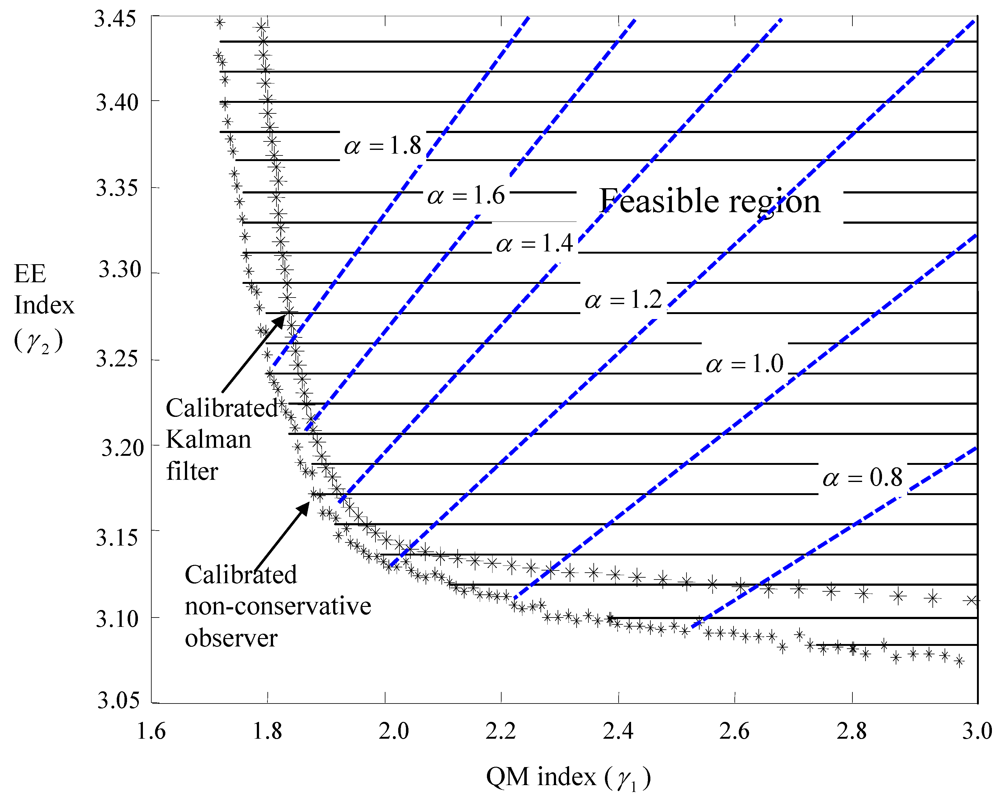
Figure 7. Improved trade-off between energy and motion objectives.

Figure 7. Improved trade-off between energy and motion objectives.

For standard mechatronic ratios of AC characteristics β = 150 and power ratings φ = 325, the ${\text{(γ}}_{\text{1}}{\text{,γ}}_{\text{2}}\text{)}$ solutions are plotted in Figure 7. It turns out that the set of feasible pairs of indexes ${\text{(γ}}_{\text{1}}{\text{,γ}}_{\text{2}}\text{)}$ is convex. Figure 7 demonstrates in non-dimensional fashion the nature of city cars: the trade-off between energy economics and quick motions. This vehicular nature has been commonly experienced, and is parameterized here. In the Figure 7, the feedbacks with calibrated non-conservative observers embedded are juxtaposed with those with calibrated Kalman-filters embedded to visualize the claimed non-conservatism.

6. Implementation of Energy-Motion Management

The procedure to implement the controller that fulfills the online energy-motion management is described as follows:

Step 1: Identify equivalent parameters of city car.

Identify, as in Section 4, the equivalent inductance L, resistance R and torque coefficient $\text{κ}$ of electric parts as well as the equivalent damping B and inertia of moment J of mechanical parts.

Step 2: Choose the mode of transient transmission.

Choose a proper mode of transient transmission with negotiation parameter $\text{α}$ in the EE-QM regulator of Figure 7, and then calculate the control dynamics of EE-QM regulation with the corresponding pair of performance indexes ${\text{(γ}}_{\text{2}}{\text{,γ}}_{\text{1}}\text{)}$. Plug the control dynamics into the dynamics in Equation (43), and then perform computer simulations with the sampling time $T$. From the computed responses prepare a set of negotiation parameters for desired transmission modes.

Step 3: Implement the transmission mode into a microcontroller.

The energy-motion regulator is then implemented into a Microchip-dsPIC chip with the Euler discretization as follows. Continuous-to-digital conversion yields:

$$\begin{array}{l}{x}_{k+1}=\mathrm{\Phi }({\omega }_j)x_k+\mathrm{\Gamma }({\omega }_j)y_k\\ u_k=\mathbf{𝓒}{x}_k\end{array}$$

(53)

where k and j are fast-time and slow-time sampling indexes, respectively. The system matrices $(\mathrm{\Phi },\mathrm{\Gamma })$ can be calculated online in a slow-time fashion; explicitly:

$$\begin{array}{c}\mathrm{\Phi }({\omega }_j)=e^{\mathbf{𝒶}({\omega }_j)}\approx {\displaystyle \sum _{i=0}^N\frac{{\mathbf{𝒶}}^i({\omega }_j)T^i}{i!}}\\ \mathrm{\Gamma }({\omega }_j)\approx T{\displaystyle \sum _{i=1}^N\frac{{\mathbf{𝒶}}^{i-1}({\omega }_j)T^{i-1}}{i!}𝔅}\end{array}$$

(54)

where $T$ is the fast-time sampling period that is short enough to make the above Taylor-series expansion accurate even with few terms, say, $N=2$ or 3 as T is 0.001 s. In the program of Equations (53) and (54), ($\mathbf{𝒶}$, $\mathrm{𝔅}$, $\mathbf{𝓒}$) are the system matrices of the integrator in series with the multi-objective LPV $L_2$-gain feedback as shown in Figure 2.

At the present time $t_k$, the dsPIC merely stores the current state $x_k$, and the update of state from $x_k$ to $x_{k+1}$ at next instant is fulfilled by the DSP-engine performing addition and multiplication of floating numbers according to Equation (53). In this sense, any time can be treated as the initial time, which makes the real-time processing as efficient as possible. Moreover, the intervals of state update are held identical to those in computer simulation, so that the real-timed operation matches the dynamics that has been verified by offline calculation, thus achieving robust implementation. At any instance, a pulse-width modulated (PWM) signal in line with the control signal u is sent to the gate-driving circuit of the switched power converter, as shown in Figure 8.

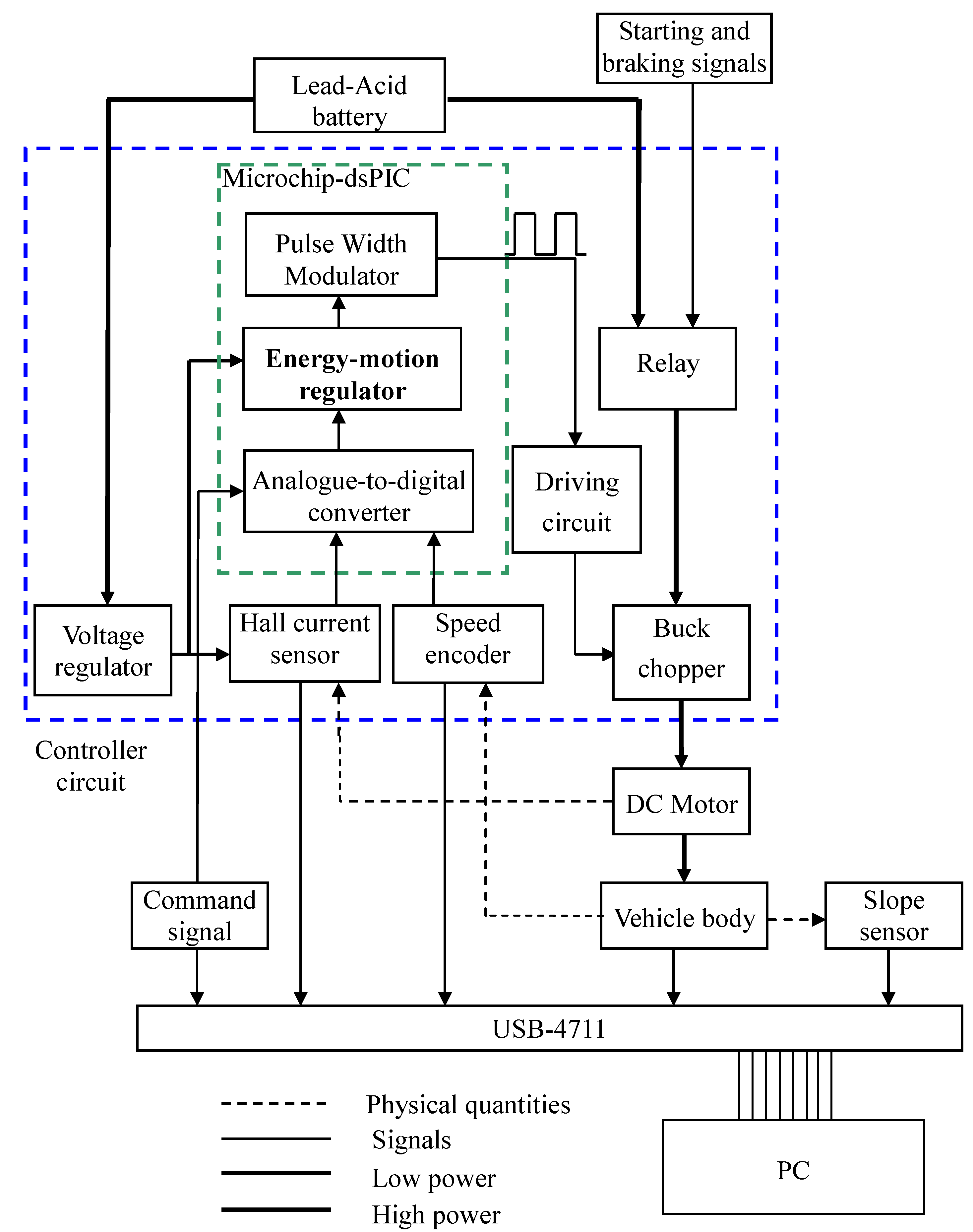
Figure 8. Means plus functions of the controller and instrumentation.

Figure 8. Means plus functions of the controller and instrumentation.

Step 4: Prepare controller circuit board.

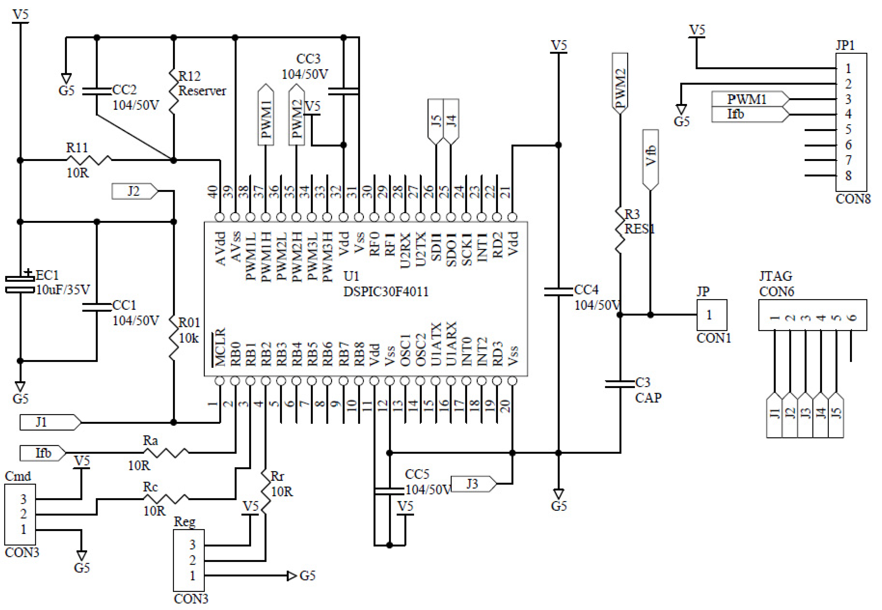
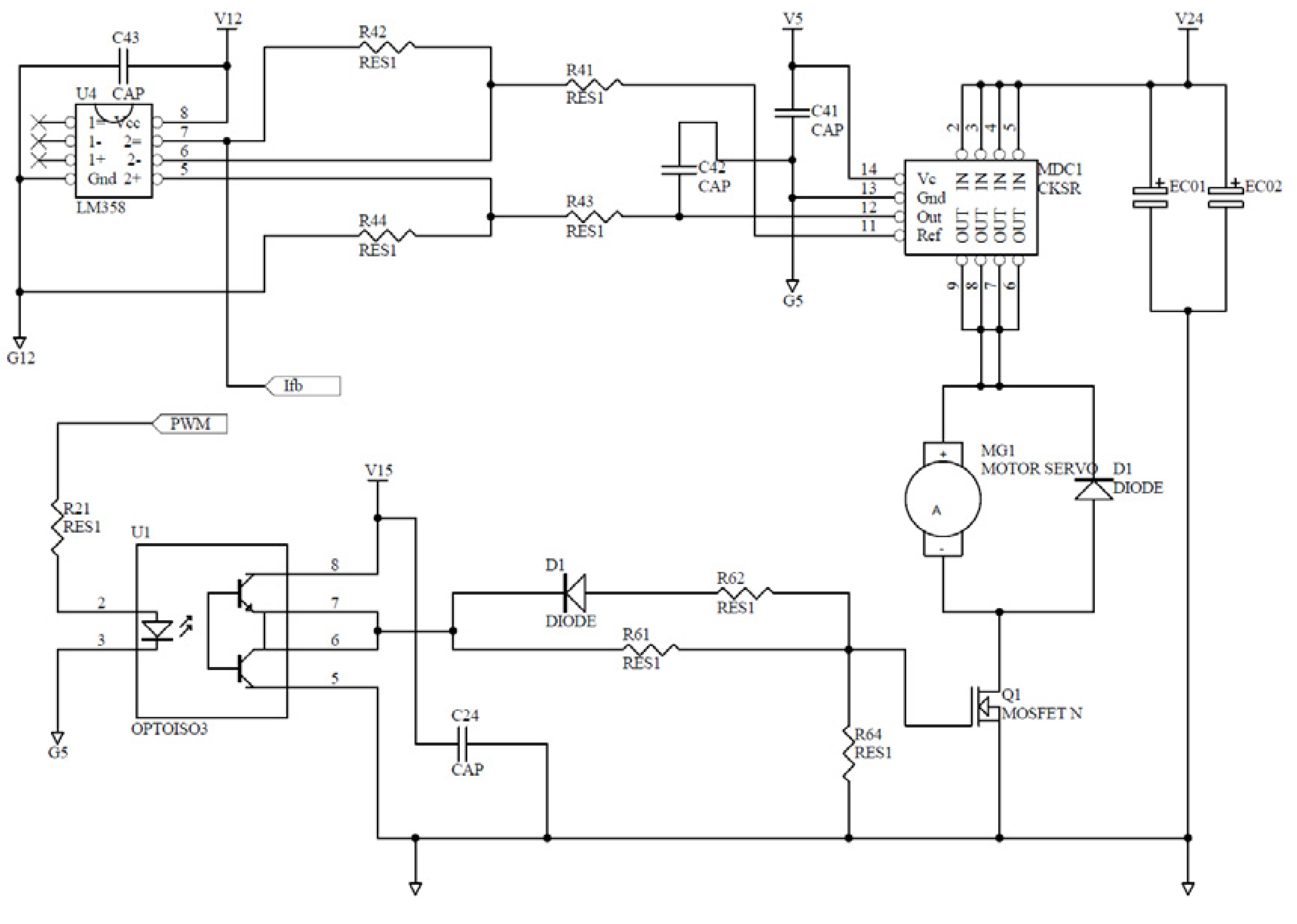
Figure 9 shows main components of the controller in design. On the circuit board are (1) a current sensor; (2) a dsPIC chip embedded with A/Ds, PWMs and the DSP programs; (3) voltage regulators; (4) switching buck choppers; (5) sensor and transducer circuits; (6) the amplification circuits driving the gates of power MOSFETs in the choppers; and (7) starting and braking relays. Figure 10 plots the auxiliary circuit of the dsPIC chip. Its reliability is known from considerable times of trials-and-errors.

Figure 9. Sensor and driver circuits in the controller.

Figure 9. Sensor and driver circuits in the controller.

Figure 10. Microchip-dsPIC auxiliary circuit in the controller.

Figure 10. Microchip-dsPIC auxiliary circuit in the controller.

7. Experimental Results and Discussion

A city car with $\overline{u}=96$V, $\overline{i}=52$A and $\overline{\text{ω}}=9200$ rpm, installing an ACS754SCB-200 Hall-effect current sensor/transducer (single bias; 0–100A input; 0–5V output) is made for these experiments. A toy DC-motor is pivoted on the axial of the motor for sensing tire speeds, and a USB4711 box is for real-timed signal acquisition of motor currents and tire speeds. The signal conditioning inside the dsPIC chip is as follows: (1) the command signal 0–5 V corresponds to the motor current 0–100 A; (2) the output of current sensor 0 V–5 V corresponds to the motor current 0–100 A; (3) the frequency of the PWM is 20 k Hz with its duty cycle 0%–100% being proportional to motor average voltage 0–96 V; and (4) the sampling time in the MIT program is $T=0.001$s.

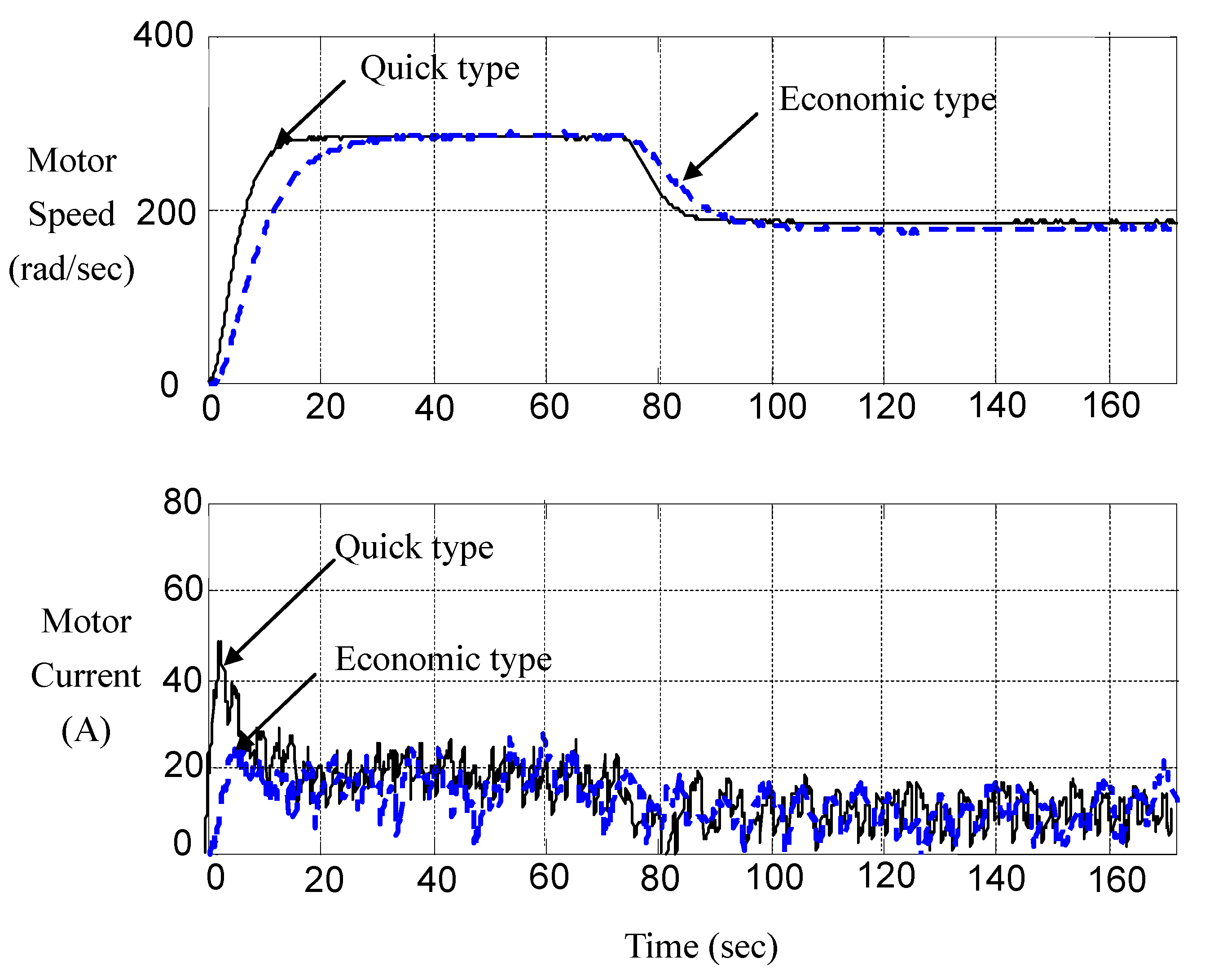
During the pilot run, we embed two modes of transient transmission into the dsPIC microcontroller to verify the multi-objective control strategy developed in Section 5. One is an economic type with the negotiation parameter $\text{α}=1.1$, and the other is a quick type with the negotiation parameter being $\text{α}=2.0$. Figure 11 records the typical response of these two types of controllers. We find that Allegro ACS754SCB-200 Hall-effect current sensor is of wide bandwidth and thus lures high-frequency noises into the loop. Though noises contaminate measurement, we can discern that the multi-objective strategy works.

Figure 11. Measured responses of economic type and quick type.

Figure 11. Measured responses of economic type and quick type.

It is more convenient to observe the responses of energy consumption per distance, especially in traffic jams, by changing the independent variable from the time t to the angular displacement θ ($\text{dθ}/\text{d}t=\text{ω}$). Accordingly, we record the responses of energy consumption, motor current and tire speed versus the angular displacement θ of the city car driven in a traffic jam in a short range and long range, respectively. Their responses of energy consumption indicate that the economic type ($\text{α}=1.1$) saves about 50% energy with respect to the quick type ($\text{α}=2.0$). 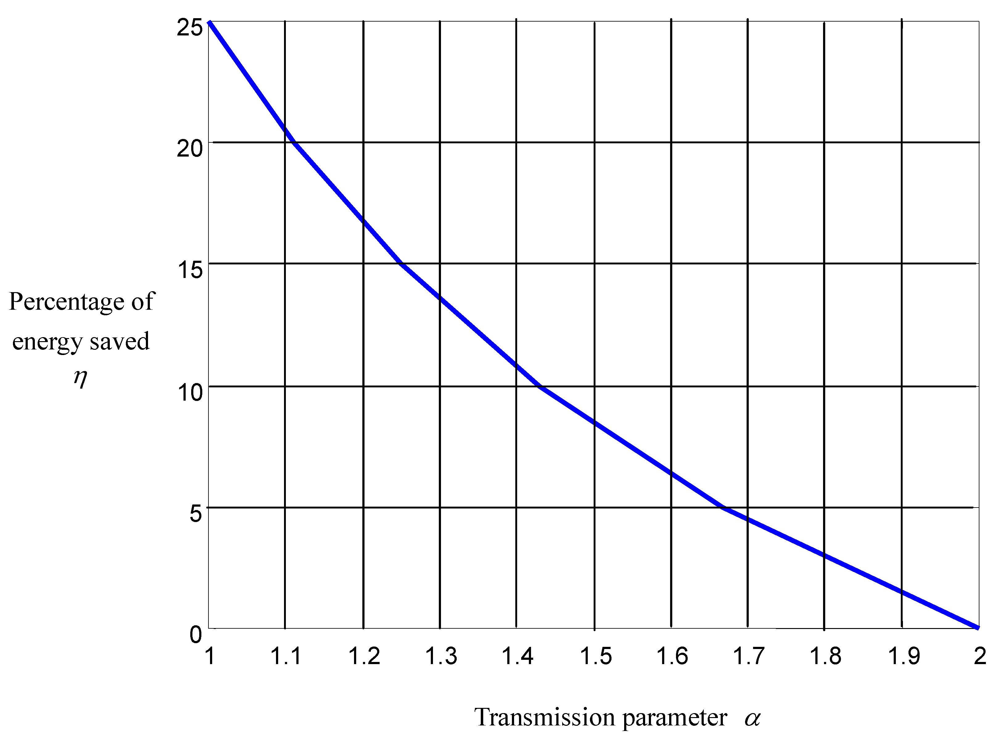Energy is saved because of reduced electric dissipation resulted from the depression of current overshoots during the acceleration and deceleration. This also protects the battery from overcharging and the DC motor from overheating, and thus saves energy. Letting the car run in the local city and accumulating data therefrom, we calculate the statistical relationship between the amount of energy being saved and the negotiation parameter, which is plotted in Figure 12. It is found that the percentage of energy saved with respect to the quick type ($\text{α}=2.0$), η, is almost inversely proportional to the negotiation parameter.

Figure 12. Energy saved versus negotiation parameter.

Figure 12. Energy saved versus negotiation parameter.

These findings correspond to our experiences: commands of rapid acceleration and deceleration tend to shorten driving ranges; however, it is usually necessary for rapid accelerations and decelerations to safely drive the car in a crowded condition. Therefore, every condition of traffic has its own mode of transient transmission when manufacturers employ our EE-QM regulator in designing controllers of city cars.

Furthermore, we record the responses of motor current and car speed when driving on level ground and uphill, respectively. On the level ground, the economic type significantly suppresses the current overshoots in transience with a bit of retard of speed. This significantly saves energy in traffic jams, when electric energy is unreasonably dissipated due to current overshoots happening during acceleration and deceleration. However, on the uphill the retardation of speed becomes significant. Then, the car should switch to the controller with a negotiation parameter large enough to climb up a steep hill. When the car is back to the level road, it should switch back to economic type to reduce energy consumption. Therefore, the negotiator parameter in transience compares to the gear ratio in steady state for regulating the EE-QM behavior, and the regulation is well captured by Figure 7, obtained by the multi-objective LPV $L_2$-gain control.

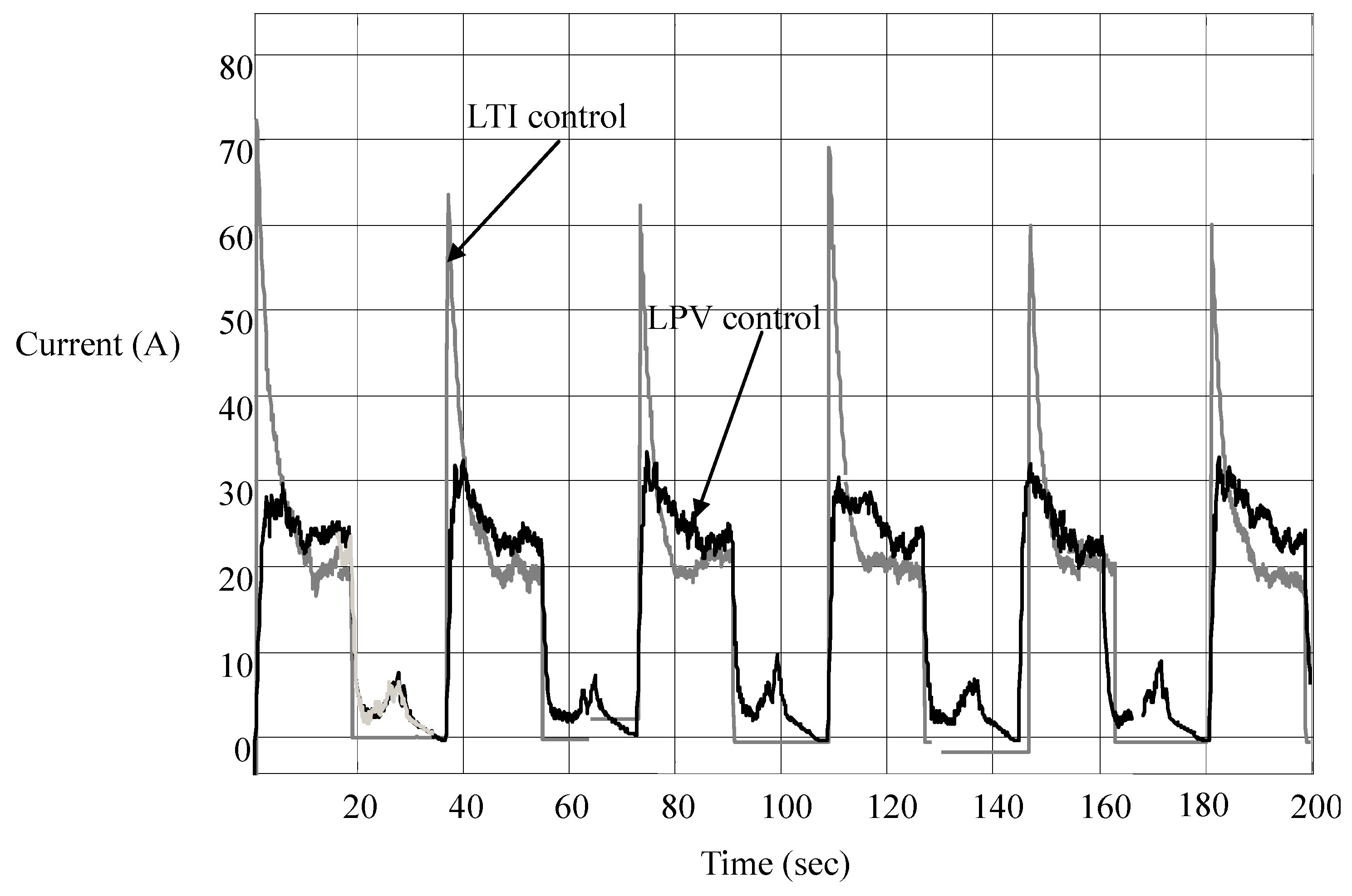
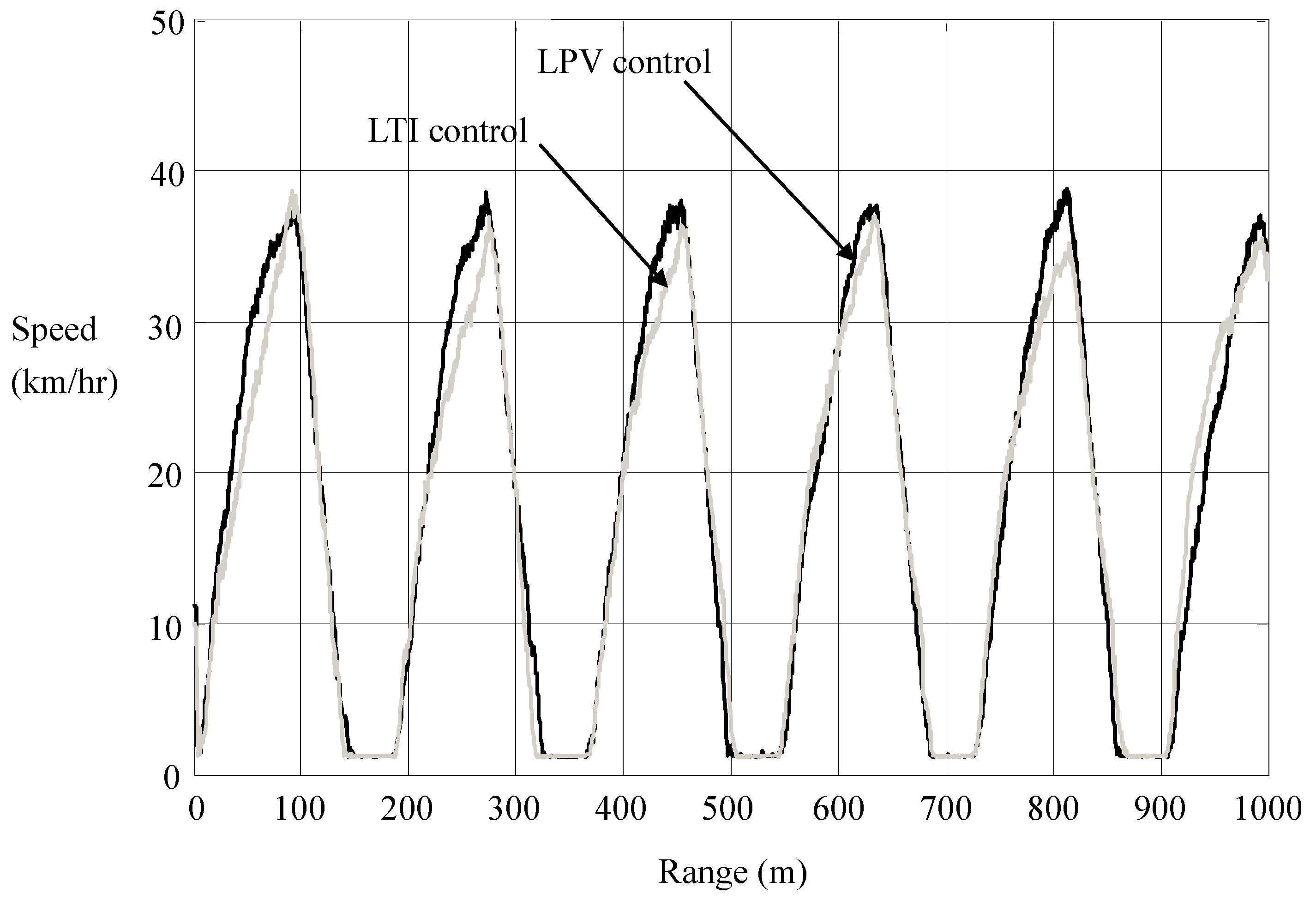
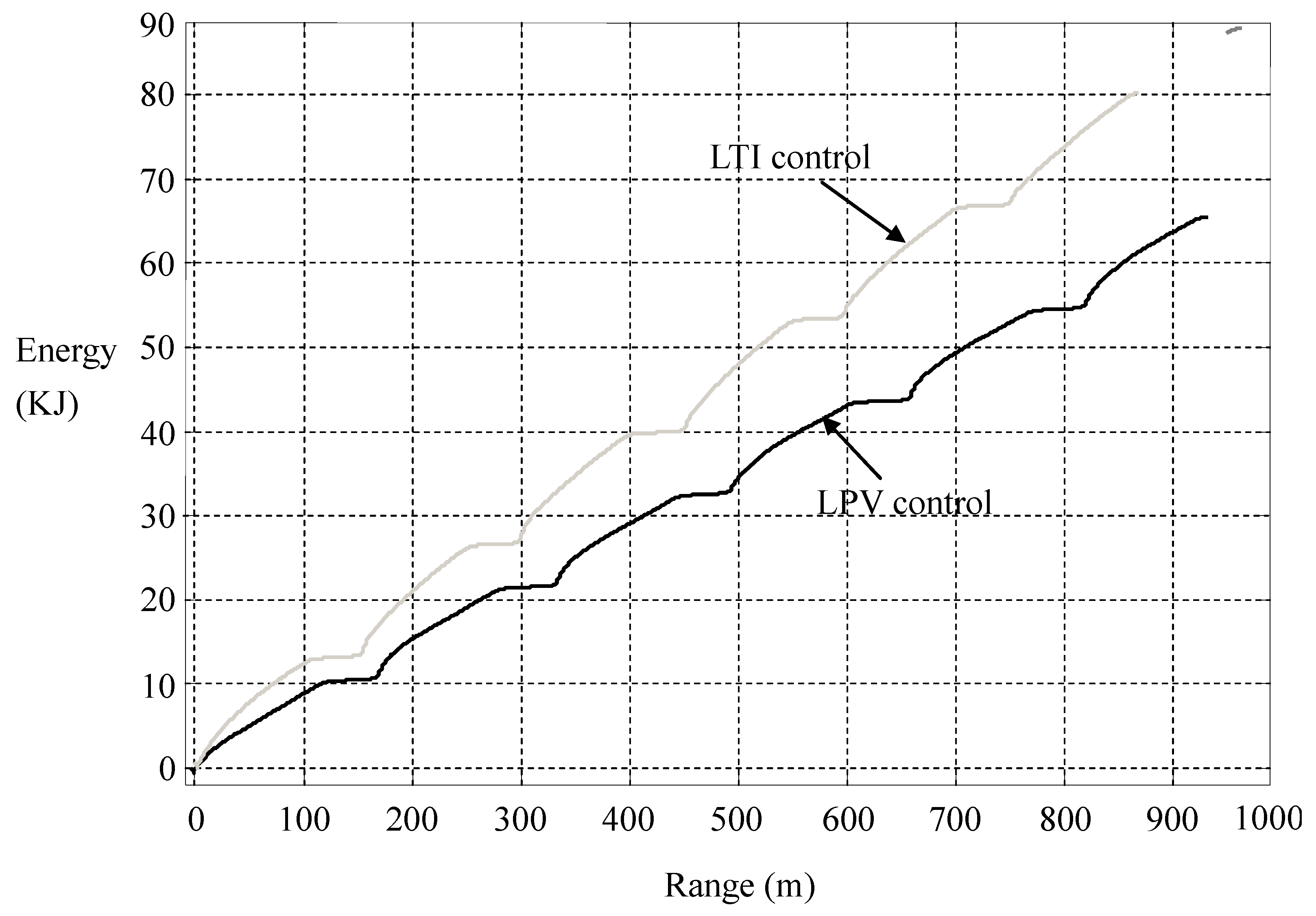
Next, we design a special road test, arranging a 1000-meter runway equipped with several stop flags. The experimental car stops at each flag, and then starts with maximum throttle up to the level speed at 40 km/h. Then, the car decelerates and stops at the next flag. We recorded the responses of motor current, tire speed, battery voltage, and PWM duty cycles to estimate the power dissipation. It is proven that per-distance control strategy has significantly better EE-QM performance than per-time control strategy, especially in a traffic jam. Experimental results are recorded in Figure 13, Figure 14 and Figure 15.

It is seen in Figure 13 that the overshoots of motor current are significantly suppressed, especially when the car is accelerated at the times of stop, say at 0 s, 36 s, 72 s, etc. That is, the per-distance control strategy not only saves energy but also protects the battery from being overcharged and power converters from being burned out. As for the small current peaks at other times, they result from small throttles needed to control the car to stop at the flags, at the times the car is running at a low speed. These peaks, large or small, have the values in line with the LPV nature of the city car, as shown in Figure 3: the equivalent resistance is almost proportional to the car speed.

Figure 13. Current responses in LTI and LPV controls.

Figure 13. Current responses in LTI and LPV controls.

We see in Figure 14 that the significant suppression of current overshoots is accompanied by a slight retardation of speed. That is, energy efficiency is achieved in transience nearly without sacrificing the time efficiency. In Figure 14, we calculate the consumption of electric energy versus the driving range, which shows that the LPV per-distance control saves a surprising amount of energy. More energy will be saved in heavier traffic.

Figure 14. Motion responses in LTI and LPV controls.

Figure 14. Motion responses in LTI and LPV controls.

Figure 15. Energy consumptions in LTI and LPV controls.

Figure 15. Energy consumptions in LTI and LPV controls.

8. Conclusions

This research work presents four prongs of knowledge regarding online energy management of city cars:

1)

The current multi-objective LPV $L_2$-gain control significantly improves the performance of energy-motion regulation.

2)

Per-distance control strategy is more suitable than per-time strategy for energy management of city cars. It spawns differential LMIs, which can be numerically solved with the finite-element approximation.

3)

The LPV parameterization can perfectly capture the nonlinear nature of DC propulsion, which provides system-level understanding to the common experience that quicker motions always give rise to larger consumption of energy.

4)

To arrive at sound energy-motion Pareto regulation, the iteration of feedback design and dynamic identification is needed.