
Map-Based Power-Split Strategy Design with Predictive Performance Optimization for Parallel Hybrid Electric Vehicles

Abstract
:1. Introduction
2. Problem Description
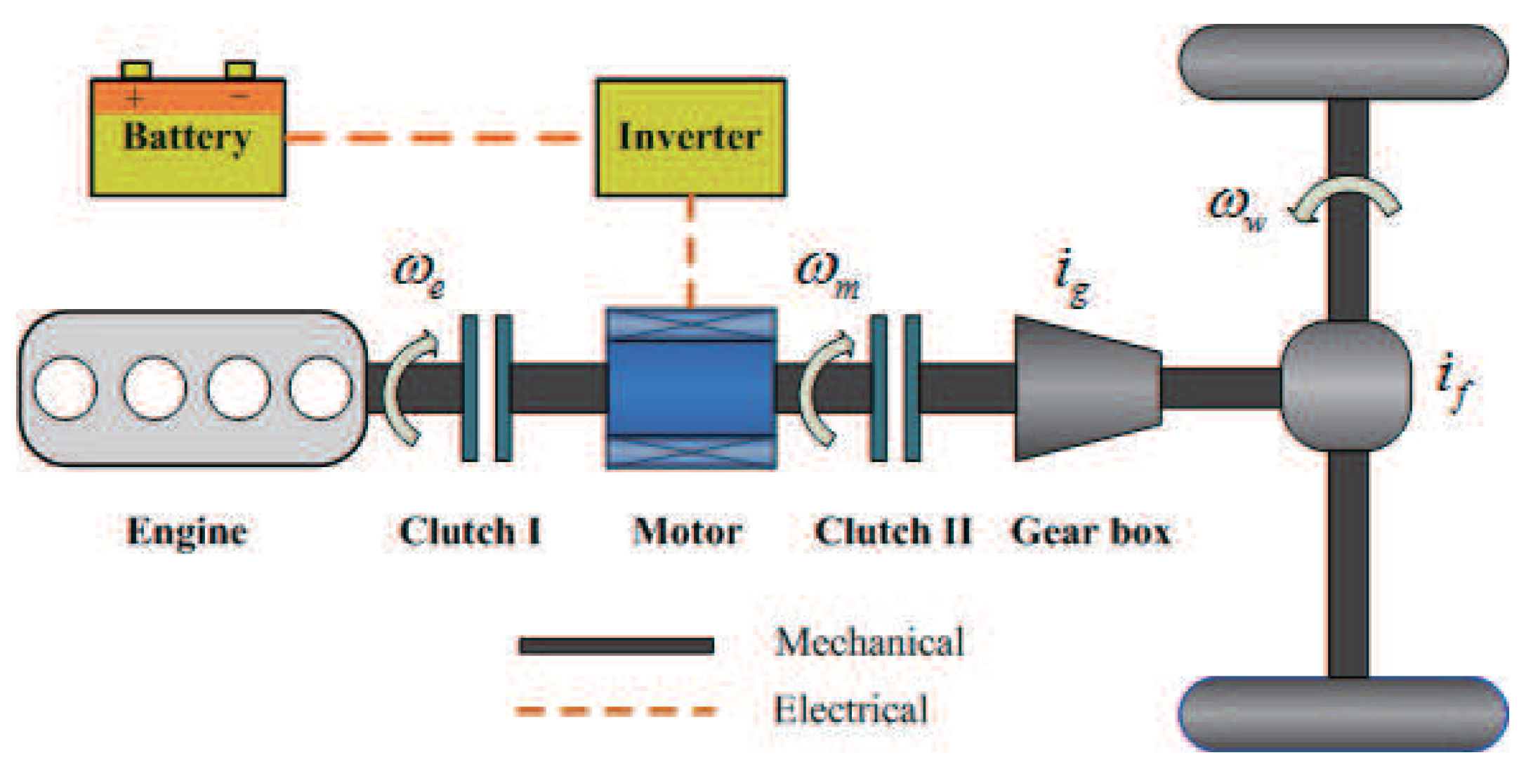
2.1. Architecture
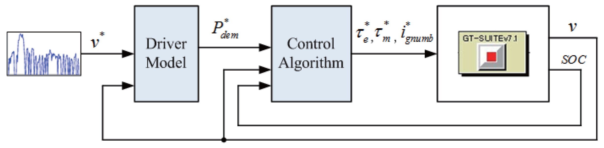
2.2. Control System Structure

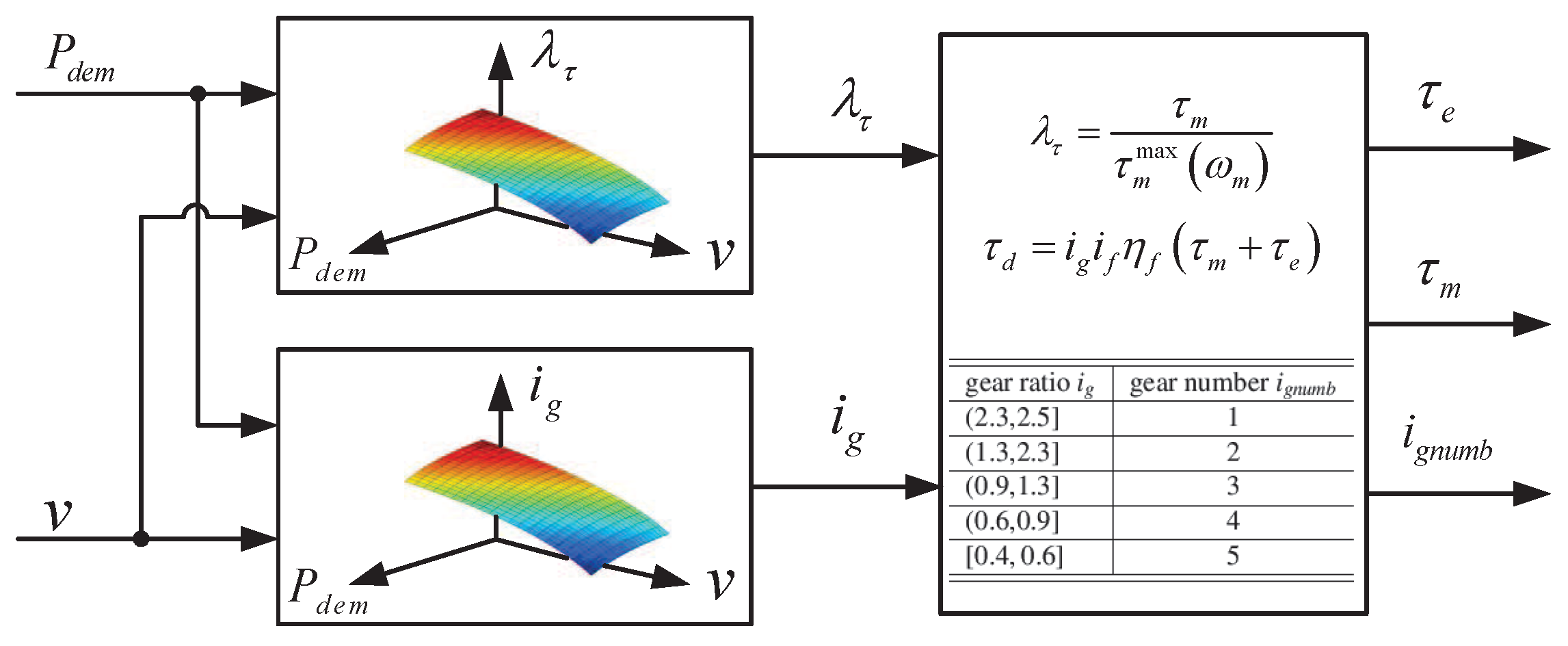
2.3. Power-Split Strategy in the HEV Mode


| Gear Ratio | Gear Number |
|---|---|
| 1 | |
| 2 | |
| 3 | |
| 4 | |
| 5 |
3. Design of Power-Split Control Maps
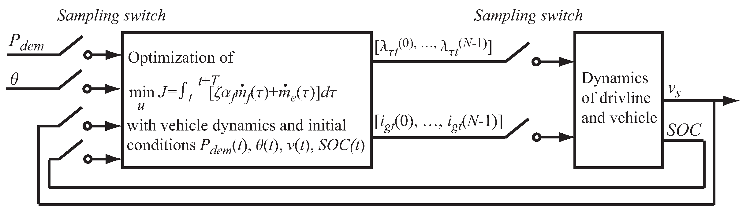
3.1. Optimal Power Split Formulation
3.2. Discrete Vehicle Model
3.3. Fuel and Electricity Consumption Model

3.4. Optimization Algorithm

4. Simulation Results and Discussion

| Vehicle Parameters | Value |
|---|---|
| Vehicle mass m | 1500 (kg) |
| Radius of the wheel | 0.32 (m) |
| Air density ρ | 1.16 (kg/m) |
| Drag coefficient | 0.3 (-) |
| Frontal area of vehicle A | 2.5 (m) |
| Coefficient of rolling resistance | 0.01 (-) |
| Final gear ratio | 5.7 (-) |
| Maximum charge capacity of the battery | 32 (Ah) |
| Open-circuit voltage of the battery | 247 (V) |
| Internal resistance of the battery | 0.12 (Ω) |


| Controller | MBOC | NMPC | Improvement | MBOC | NMPC | Improvement | MBOC | NMPC | Improvement |
|---|---|---|---|---|---|---|---|---|---|
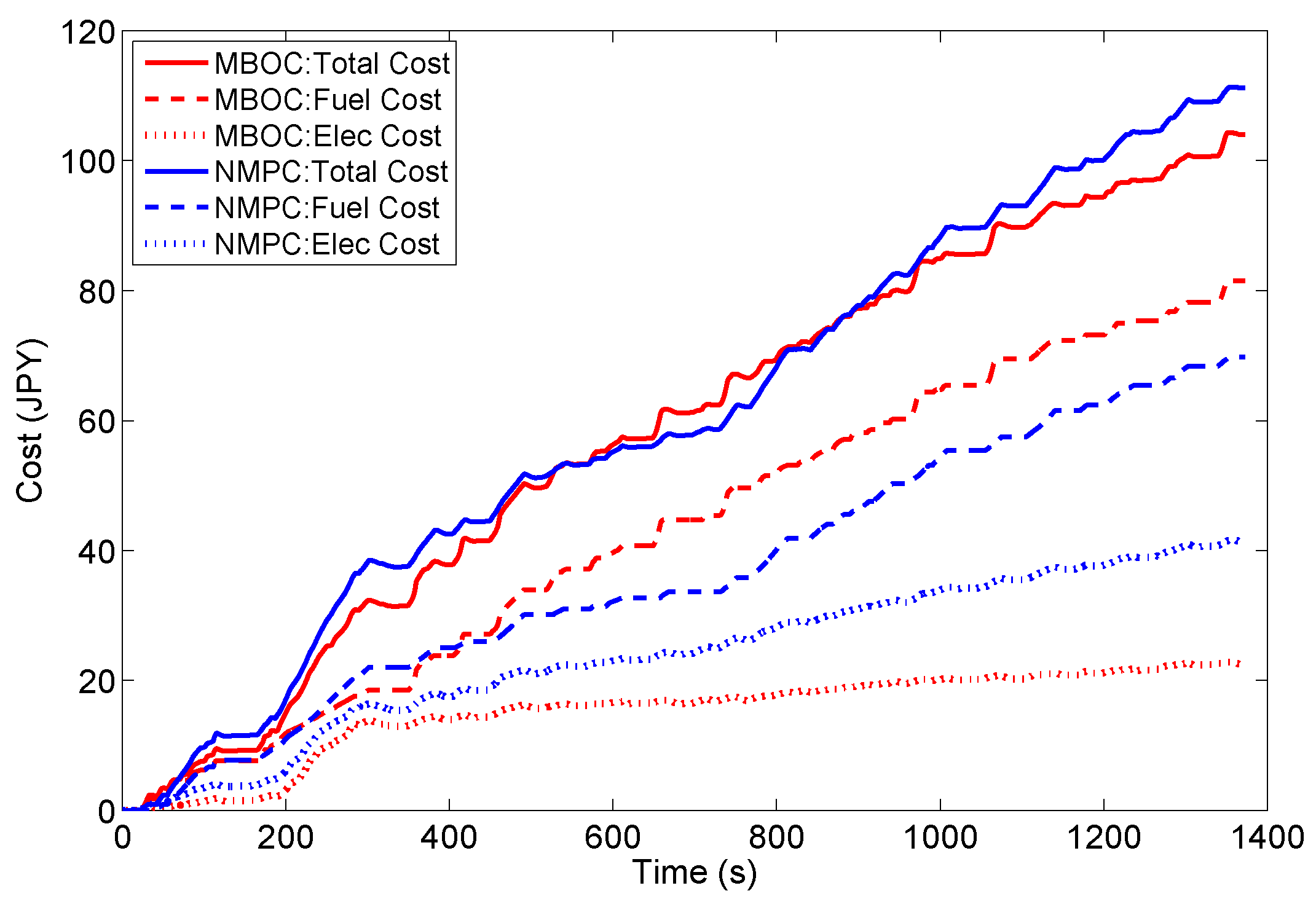
| Fuel Cost (JPY) | 81.5 | 69.7 | −16.9% | 78.6 | 70.5 | −11.5% | 97.4 | 87.6 | −11.2% |
| Electricity Cost (JPY) | 22.5 | 41.5 | +45.8% | 32.8 | 50.2 | +34.7% | 29.2 | 65.0 | +55.1% |
| Total Cost (JPY) | 104.0 | 111.2 | +6.5% | 111.4 | 120.7 | +7.7% | 126.6 | 152.6 | +17.0% |
| Energy Price Ratio | |||
|---|---|---|---|
| Fuel consumption (g) | 407.4 | 393.0 | 487.0 |
| Electricity consumption (kWh) | 1.127 | 1.093 | 0.583 |
| Total consumption (MJ) | 18.72 | 13.37 | 9.11 |
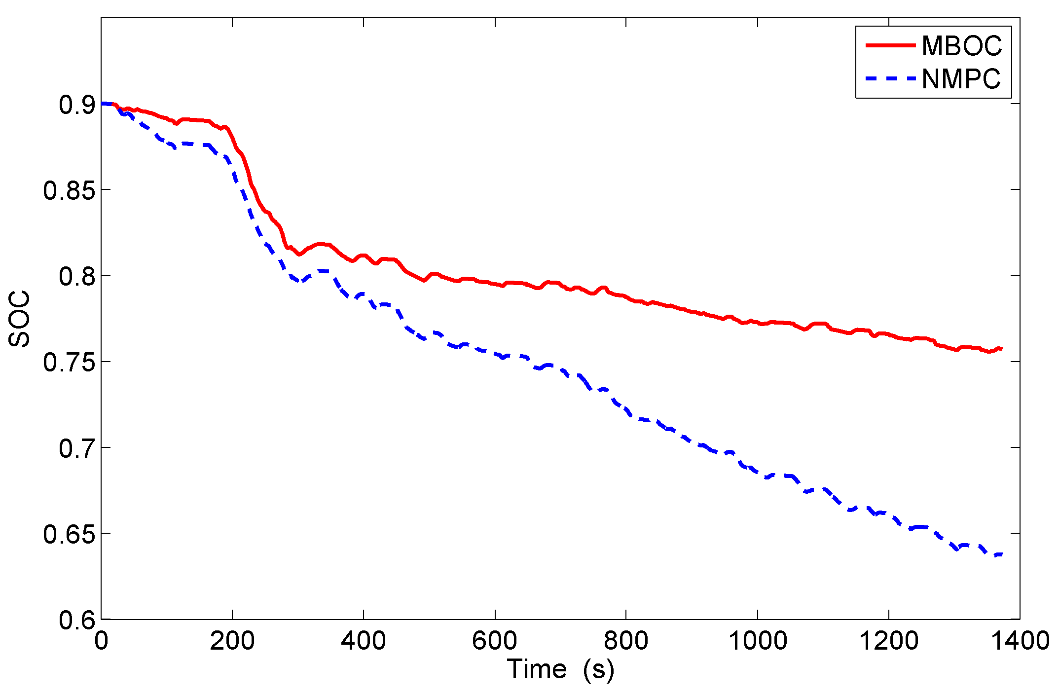
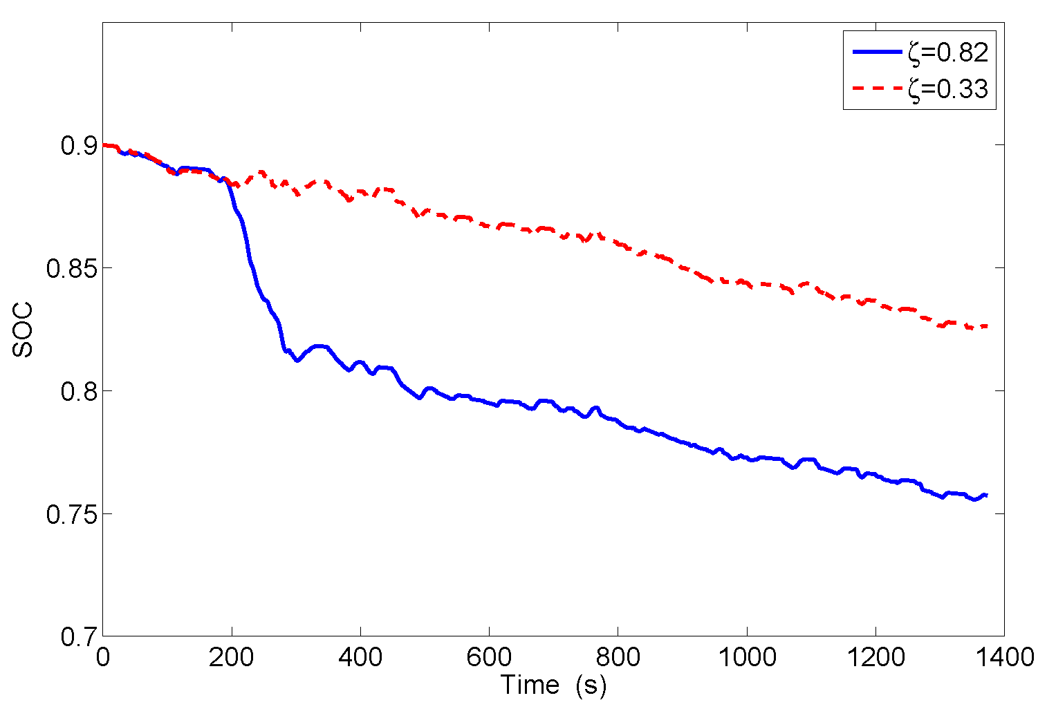
| Terminal SOC (-) | 0.757 | 0.762 | 0.826 |


5. Conclusions
Conflicts of Interest
Abbreviations
| EV | Electric vehicle | |
| FCEV | Fuel cell electric vehicle | |
| HEV | Hybrid electric vehicle | |
| PHEV | Plug-in hybrid electric vehicle | |
| DP | Dynamical programming | |
| SOC | State of charge | |
| MPC | Model predictive control | |
| EM | Electric machine | |
| ICE | Internal combustion engine | |
| BR | Battery recover | |
| BSFC | Break specific fuel consumption | |
| SQP | Sequential quadratic programming | |
| QP | Quadratic programming | |
| UDDS | Urban dynamometer driving schedule | |
| NMPC | Nonlinear model predictive control | |
| MBOC | Map-based optimal control | |
| GMRES | Generalized minimum residual |
References
- Katrašnik, T. Hybridization of powertrain and downsizing of IC engine—A way to reduce fuel consumption and pollutant emission—Part I. Energy Convers. Mang. 2007, 48, 1411–1423. [Google Scholar] [CrossRef]
- Matthé, R.; Eberle, U. The voltec system-energy storage and electric propulsion. In Lithium-Ion Batteries; Pistoia, G., Ed.; Elsevier: Amsterdam, The Netherlands, 2014; pp. 151–176. [Google Scholar]
- Tanoue, K.; Yanagihara, H.; Kusumi, H. Hybrid is a key technology for future automobiles. In Hydrogen Technology; Léon, A., Ed.; Springer: Berlin, Germany, 2008; pp. 235–272. [Google Scholar]
- Stephen, C.H.; Sullivan, J. Environmental and energy implications of plug-in hybrid-electric vehicle. Environ. Sci. Technol. 2008, 42, 1185–1190. [Google Scholar] [CrossRef]
- Chau, K.T.; Wong, Y.S. Overview of power management in hybrid electric vehicles. Energy Convers. Mang. 2002, 43, 1953–1968. [Google Scholar] [CrossRef]
- Wirasingha, S.G.; Emadi, A. Classification and review of control strategies for plug-in hybrid electric vehicle. IEEE Trans. Veh. Technol. 2011, 60, 111–122. [Google Scholar] [CrossRef]
- Serrao, L.; Onori, S.; Rizzoni, G. A comparative analysis of energy management strategies for hybrid electric vehicles. J. Dyn. Syst. Meas. Control 2011, 133, 1–9. [Google Scholar] [CrossRef]
- Banvait, H.; Anwar, S.; Chen, Y. A rule-based energy management strategy for plug-in hybrid electric vehicle(PHEV). In Proceedings of the American Control Conference, St. Louis, MO, USA, 10–12 June 2009.
- Abdelsalam, A.A.; Cui, S. A fuzzy logic global power management strategy for hybrid electric vehicles based on a permanent magnet electric variable transmission. Energies 2012, 80, 1175–1198. [Google Scholar] [CrossRef]
- Trovão, J.P.; Pereirinha, P.G.; Jorge, H.M.; Antunes, C.H. A multi-level energy management system for multi-source electric vehicles-An integrated rule-based meta-heuristic approach. Appl. Energy 2013, 105, 304–318. [Google Scholar] [CrossRef]
- Jalil, N.; Kheir, N.A.; Salman, M. Rule-based energy management strategy for a series hybrid vehicle. In Proceedings of the American Control Conference, Albuquerque, MI, USA, 6 June 1997.
- Schouten, N.J.; Salman, M.A.; Kheir, N.A. Fuzzy logic control for parallel hybrid vehicles. IEEE Trans. Control Syst. Technol. 2002, 10, 460–468. [Google Scholar] [CrossRef]
- Sharer, P.B.; Rousseau, A.; Karbowski, D.; Pagerit, S. Plug-in hybrid electric vehicle control strategy: Comparison between EV and charge-depleting options. Technical Paper 2008-01-0460. In Proceedings of the SAE, Detroit, MI, USA, 14–17 April 2008.
- Pisu, P.; Rizzoni, G. A comparative study of supervisory control strategies for hybrid electric vehicles. IEEE Trans. Control Syst. Technol. 2007, 15, 506–518. [Google Scholar] [CrossRef]
- Nüesch, T.; Elbert, P.; Flankl, M.; Onder, C.; Guzzella, L. Convex optimization for the energy management of hybrid electric vehicles considering engine start and gearshift costs. Energies 2014, 7, 834–856. [Google Scholar] [CrossRef]
- Hou, C.; Ouyang, M.; Xu, L.; Wang, H. Approximate pontryagin’s minimum principle applied to the energy management of plug-in hybrid electric vehicles. Appl. Energy 2014, 115, 174–189. [Google Scholar] [CrossRef]
- Larsson, V.; Johannesson Mårdh, L.; Egardt, B.; Karlsson, S. Commuter route optimized energy management of hybrid electric vehicles. IEEE Trans. Intell. Transp. Syst. 2014, 15, 1145–1154. [Google Scholar] [CrossRef]
- Lin, C.C.; Peng, H.; Grizzle, J.W.; Kang, J.M. Power management strategy for a parallel hybrid electric truck. IEEE Trans. Control Syst. Technol. 2003, 11, 839–849. [Google Scholar]
- Moura, S.J.; Fathy, H.K.; Callaway, D.S.; Stein, J.L. A stochastic optimal control approach for power management in plug-in hybrid electric vehicles. IEEE Trans. Control Syst. Technol. 2011, 19, 545–555. [Google Scholar] [CrossRef]
- Gong, Q.; Li, Y.; Peng, Z.R. Trip-based optimal power management of plug-in hybrid electric vehicles. IEEE Trans. Veh. Technol. 2008, 57, 3393–3401. [Google Scholar] [CrossRef]
- Scordia, J.; Desbois-Renaudin, M.; Trigui, R.; Jeanneret, B.; Badin, F.; Plasse, C. Global optimization of energy management laws in hybrid vehicles using dynamic programming. Int. J. Veh. Des. 2005, 39, 349–367. [Google Scholar] [CrossRef]
- Moura, S.J.; Callaway, D.S.; Fathy, H.K.; Stein, J.L. Tradeoffs between battery energy capacity and stochastic optimal power management in plug-in hybrid electric vehicles. J. Power Sources 2010, 195, 2979–2988. [Google Scholar] [CrossRef]
- Sciarretta, A.; Guzzella, L. Control of hybrid electric vehicles. IEEE Control Syst. Mag. 2007, 27, 60–70. [Google Scholar] [CrossRef]
- Sundstrom, O.; Guzzella, L.; Soltic, P. Torque-assist hybrid electric powertrain sizing: from optimal control towards a sizing law. IEEE Trans. Control Syst. Technol. 2010, 18, 837–849. [Google Scholar] [CrossRef]
- Tulpule, P.; Marano, V.; Rizzoni, G. Effect of traffic, road and weather information on phev energy management. Technical Paper 2011-24-0162. In Proceedings of the SAE, Detroit, MI, USA, 12–14 April 2011.
- Borhan, H.; Vahidi, A.; Phillips, A.M.; Kuang, M.L.; Kolmanovsky, I.V.; di Cairano, S. MPC-based energy management of a power-split hybrid electric vehicle. IEEE Trans. Control Syst. Technol. 2012, 20, 593–603. [Google Scholar] [CrossRef]
- Yan, F.; Wang, J.; Huang, K. Hybrid electric vehicle model predictive control torque-split strategy incorporating engine transient characteristic. IEEE Trans. Veh. Technol. 2012, 61, 2458–2467. [Google Scholar] [CrossRef]
- Zhang, J.Y.; Shen, T.L. Nonlinear MPC-based power-assist scheme of internal combustion engines in plug-in hybrid electric vehicles. In Proceedings of the European Control Conference, Strasbourg, France, 24–27 June 2014.
- Bemporad, A.; Morari, M.; Dua, V.; Pistikopoulos, E.N. The explicit linear quadratic regulator for constrained systems. Automatica 2002, 38, 3–20. [Google Scholar] [CrossRef]
- Bemporad, A.; Borrelli, F.; Morari, M. Model predictive control based on linear programming—The explicit solution. IEEE Trans. Automat. Control 2002, 47, 1974–1985. [Google Scholar] [CrossRef]
- Ohtsuka, T. A continuation/GMRES method for fast computation of nonlinear receding horizon control. Automatica 2004, 40, 563–574. [Google Scholar] [CrossRef]
- Richter, S.; Jones, C.N.; Morari, M. Computational complexity certification for real-time MPC with input constraints based on the fast gradient method. IEEE Trans. Automat. Control 2012, 57, 1391–1403. [Google Scholar] [CrossRef]
- Marsden, J.E.; West, M. Discrete mechanics and variational integrators. Acta Numer. 2011, 10, 357–514. [Google Scholar] [CrossRef]
- Chyba, M.; Hairer, E.; Vilmart, G. The role of symplectic intergrators in optimal control. Optim. Control Appl. Methods 2009, 30, 367–382. [Google Scholar] [CrossRef] [Green Version]
- Van Mierlo, J.; Van den Bossche, P.; Maggetto, G. Models of energy sources for EV and HEV: fuel cells, batteries, ultracapacitors, flywheels and engine-generators. J. Power Sources 2004, 128, 76–89. [Google Scholar] [CrossRef]
- Rizzoni, G.; Guzzella, L.; Baumann, B.M. Unified modeling of hybrid electric vehicle drivetrains. IEEE-ASME Trans. Mech. 1999, 4, 246–257. [Google Scholar] [CrossRef]
- Gill, P.E.; Murray, W.; Wright, M.H. Practical Optimization; Academic Press: London, UK, 1982. [Google Scholar]
- Boggs, P.T.; Tolle, J.W. Sequential Quadratic Programming. Acta Numer. 1995, 4, 1–51. [Google Scholar] [CrossRef]
- Zhang, J.Y.; Shen, T.L.; Sawada, T.; Kubo, M. Nonlinear MPC-based power management strategy for plug-in parallel hybrid electrical vehicles. In Proceedings of the Chinese Control Conference, Nanjing, China, 28–30 July 2014.
© 2015 by the authors; licensee MDPI, Basel, Switzerland. This article is an open access article distributed under the terms and conditions of the Creative Commons Attribution license (http://creativecommons.org/licenses/by/4.0/).
Share and Cite
Fan, J.; Zhang, J.; Shen, T. Map-Based Power-Split Strategy Design with Predictive Performance Optimization for Parallel Hybrid Electric Vehicles. Energies 2015, 8, 9946-9968. https://doi.org/10.3390/en8099946
Fan J, Zhang J, Shen T. Map-Based Power-Split Strategy Design with Predictive Performance Optimization for Parallel Hybrid Electric Vehicles. Energies. 2015; 8(9):9946-9968. https://doi.org/10.3390/en8099946
Chicago/Turabian StyleFan, Jixiang, Jiangyan Zhang, and Tielong Shen. 2015. "Map-Based Power-Split Strategy Design with Predictive Performance Optimization for Parallel Hybrid Electric Vehicles" Energies 8, no. 9: 9946-9968. https://doi.org/10.3390/en8099946