An Application of Spectral Kurtosis to Separate Hybrid Power Quality Events

Abstract

For the development of the future smart grid, the detection of power quality events is a key issue for the power system monitoring. Voltage sags, swells, harmonics (variations) and interruptions, which produce large losses for commercial and industrial consumers, are the main events to be considered due to the sensitivity of equipment to these electrical anomalies. The steady-state events are even more frequently accompanied by transients, the discrimination and localization being far more exigent and requiring advanced signal separating tools to be incorporated in the measurement equipment. This paper shows the event detection performance of the spectral kurtosis as a signal separating tool in the frequency domain. The disturbances under test are hybrid signals resulting from the coupling between amplitude defects and non-desired higher frequencies. Being a fourth-order spectrum, the kurtosis is confirmed as a noise-resistant tool that enhances impulsiveness, therefore characterizing the electrical anomalies. In the beginning of the analysis, the voltage sag is established as a reference; then, the disturbances (oscillatory transients and harmonics) are coupled at the starting and ending instants of the sag, resulting in complex hybrid events. The results show that the spectral kurtosis enhances the detection of both types of events (steady state and transients), which are outlined in a bump shape in the fourth-order frequency pattern and centered in the main carrier frequency. Indeed, while the oscillatory transients are associated with softer and lower-amplitude peaks, the harmonics correspond to crisper and higher ones. As these mixed electrical faults are very common in the actual power grid, the article postulates the higher-order spectra to be implemented in prospective online measurement instruments.

1. Introduction

With the uncontrolled growth of society, the consequent energy demand forces drastically adapting the power grid topology. Examples of this change are electric and hybrid cars, which suppose important loads in the power system, and nowadays, they are widely introduced [1,2].

In order to protect the environment, big fossil fuel power plants are being replaced by small renewable energies generators, which suppose enormous implications for the environment and for the power grid. A big synchronous power generator, as can be found in an average power plant, delivers a perfect sinusoidal waveform. In addition, any wave distortion is compensated and converted into a perfect waveform, and it can correct some grid outbalances by generating or consuming reactive power.

At the same time, the power grid is turning into a meshed system. This configuration allows the distribution system to prevent faults, creating new alternate routes for the power flow. In addition, using the information of power generated and consumed in any node and the grid characteristics, it can be configured to minimize losses. However, this has implications when a disturbance occurs. In a mesh system, many lines are connected to any node. In this situation, when a disturbance takes place at a point, it will leave all of the lines connected to that node, expanding quickly through the power grid.

Evolution of the topology of a high voltage power grid could be seen in [3]; the effects of different topologies in a normal function are explained in [4]; and an idea of the complexity level reached by the power gird is given in [5]. All of these complex network schemes require changes in the control, as seen in [6], which implies more elements in the grid. Any additional element could introduce disturbances in the case of a fault.

Collaterally, the new advantages in electrical power generation and power distribution systems have led to a power quality (PQ) degradation. Equipment, such as transformers, motors or conductors, undergo overload and generate low PQ conditions, due to harmonics, insufficient voltage, oscillatory transients or other disturbances. Due to the shared responsibility of PQ, it is important to monitor the voltage and currents at the connection point and in the low, medium and high voltage grid.

One of the most important PQ disturbances is the sag or voltage dip, explained and regulated in [7]. It consists of a reduction of the amplitude value with a duration from a half cycle to a few minutes. Changes in the amplitude usually occur suddenly and carry coupled disturbances: oscillatory transients and temporal harmonic distortions are common during or after amplitude transitions. All of those disturbances are examined and explained carefully by IEEE in [8]. Because the amplitude change in the base waveform is usually higher, coupled disturbances are difficult to detect.

In this frame, this work postulates the spectral kurtosis (SK) as a computing tool to detect and characterize transient disturbances that are coupled to steady-state sags. The capabilities of higher-order statistics (HOS) to enhance impulsiveness (non-Gaussian behavior) have been formerly proven in some fields and areas of science and technology [9,10,11,12,13,14,15,16]. More precisely, in the field of the PQ characterization, the research team has developed intelligent methods to detect power quality events, using HOS in the time and frequency domains [17,18,19].

Regarding direct backgrounds of HOS applications in this field, in the time-domain, several notable works are worthy, e.g., Bollen et al. introduced new statistical features to PQ event detection [20]. In the same direction, Gu and Bollen [21] found relevant characteristics associated with PQ events in the time and frequency domains. The work by Ribeiro et al. [22] is also remarkable, which extracted new time-domain features based on cumulants. The same authors performed the classification of single and multiples disturbances using HOS in the time domain and Bayes’ theory-based techniques [23]. HOS techniques and estimators have also been implemented to specifically detect sags and swells [24]. The categorization of PQ anomalies had been formerly performed by Nezih and Ece in [25], where they proved that HOS and quadratic classifiers improve the second order-based methods. The most aligned work is the one developed by Liu et al. in [26], where the researchers extracted a rich set of higher-order features related to the analysis as different types of PQ events using spectral kurtosis.

The paper is structured as follows. Firstly, the SK procedure is explained in Section 2, then coupled disturbances are examined using the SK analysis in the Section 3. Finally, conclusions are drawn in Section 4.

2. The Spectral Kurtosis: Procedure of Analysis

The SK is a fourth-order spectrum that deals with the peakedness of the probability density function associated with a measurement data series. From a practical point of view, the traditional power spectrum does not reflect these impulsive features of the time series, which indeed constitute the key attributes of PQ events. For that reason, the SK pattern should reflect the transient characteristics associated with the frequencies under test [12].

The procedure of computation is explained as follows. The time domain register is chopped into realizations or segments overlapped by 50%. This means that the second half of a time realization is the first half of the next realization. Then, the FFT of each realization is calculated and stored in a matrix, where every new FFT is added in a new row. With the data presented this way, Equation (1) represents the estimator involved in the SK computation:

$${\widehat{G}}_{2,X}^{N,M}\left(m\right)=\frac{M}{M-1}\left[\frac{\left(M+1\right){\sum }_{i=1}^M{\left|X_N^i\left(m\right)\right|}^4}{{\left({\sum }_{i=1}^M{\left|X_N^i\left(m\right)\right|}^2\right)}^2}-2\right]$$

(1)

where X is the FFT matrix, in which the upper index i means the row (realization) and the index m is associated with the column (frequency). M realizations with N points have been considered. The final SK vector has the same points as the FFT vector; equal to $N/2$. The more realizations are involved in the calculation, the more precise is this procedure. However, the computational load increases with the size and the number of realizations, so a correct size and number of points must be indicated for the realizations to achieve suitable resolution and precision, but with an acceptable computational burden; in this case, 1000 realizations of 0.1 s each, using a sampling frequency of 20,000 Hz for all analysis. This means an SK vector of 1000 points and a maximum frequency of 10,000 Hz.

As said formerly, 1000 realizations of 0.1 s are needed; however, each register has only a 1-s length. This problem is overcome using a sliding version for the SK estimator. The spectral data are accumulated for 100 s before the SK could be calculated.

Hereinafter, the results are presented, dividing them into groups corresponding to different types of electrical perturbations.

3. Coupled Disturbances

In this section, an evolution to a coupled signal will be done. Firstly, the base response for a healthy signal will be set. Then, the sag will be examined alone, and finally, a sag with an oscillatory transient and harmonic distortion coupled is studied.

Firstly, and with the goal of getting a reference, the analysis of a healthy signal is performed (shown in Figure 1). The healthy condition is stated as a sinusoid of unitary amplitude. It will be the base amplitude assumed throughout the work.

With the frequency pattern characterization of this ideal signal, the anomalies associated with the disturbances are detected more easily. Synthetics are used in order to control all of the signal parameters, allowing in this way a correct comparison among them. In order to introduce real-life conditions, additive Gaussian noise with a standard deviation (σ) of 0.05 is added to all signals.

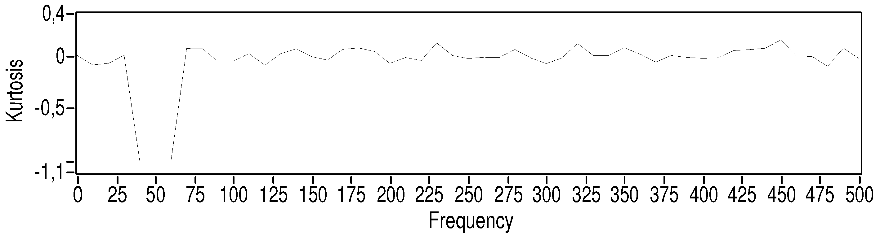
Figure 1. Spectral kurtosis (SK) analysis over a healthy signal. SK results corresponding to a 50-Hz sinusoid with additive Gaussian noise with (σ = 0.05), swept from 0 to 500 Hz.

Figure 1. Spectral kurtosis (SK) analysis over a healthy signal. SK results corresponding to a 50-Hz sinusoid with additive Gaussian noise with (σ = 0.05), swept from 0 to 500 Hz.

Signals have been synthesized with the same properties as described in the SK definition, i.e., 20,000 samples per second. That means a maximum frequency of 10,000 Hz for the SK analysis. However, the graph only shows up to 500 Hz. In the graph, the same response from 100 to 500 Hz can be seen. It continues equally for the rest of the frequencies. As no new information could be extracted from frequencies higher than 500 Hz, only frequencies under that value are shown, obtaining in this way a more detailed representation. Hereinafter, this is performed for all experiments, due to all frequencies involved in the considered disturbances being lower than 500 Hz.

In Figure 1, the same pattern is outlined for almost all of the frequencies. These are small variations around the zero, with a maximum deviation of 0.2. This value is related to the additive noise, which is rejected by the SK. In the lower frequency band of the graph, a −1-valued peak appears, centered at a frequency of 50 Hz. With a discrete spectral resolution of 10 Hz, the −1 value copes with the frequencies of 40 and 60 Hz. This zone is associated with the power signal frequency and indicates the feature associated with a constant amplitude signal.

Being a higher-order spectrum, the SK is postulated as a noise-resistant analysis tool. This property is tested studying different noise contamination levels. Table 1 shows the kurtosis values for the base frequency (50 Hz) and maximum variation around zero for the rest of the spectrum for Gaussian additive noise with σ from 0.05 to 0.80. If a 50-Hz kurtosis value is examining, no important change could be observed. As noise contamination increases, kurtosis takes values a litter higher, from −0.99998 to −0.9962. However, in this range, all could be considered −1, with an error lower than 1%. In relation to the maximum variation around zero, there are no relations with the noise contamination. Different values could be seen for different contamination levels, with a maximum value of 0.345210 and a minimum value of 0.206976. As a test of the randomness of these values, 1000 analyses with the σ = 0.05 condition have been performed. Each single analysis has returned a different maximum variation value around zero, the higher one being 0.417784 (only in two analyses) and the lower one 0.177371 (in some of them). The average value obtained in this experiment is 0.25.

Table 1. SK analysis results for a healthy signal with different noise contamination levels.

Noise level (σ)	50-Hz Peak value	Maximum variation around zero
0.05	−0.999986	0.250188
0.10	−0.999937	0.209871
0.15	−0.999866	0.251025
0.20	−0.999761	0.206976
0.25	−0.999599	0.234948
0.30	−0.999480	0.210391
0.35	−0.999311	0.259246
0.40	−0.999089	0.213317
0.50	−0.998368	0.263187
0.60	−0.997846	0.345210
0.70	−0.997300	0.216441
0.80	−0.996223	0.238456

Table 1. SK analysis results for a healthy signal with different noise contamination levels.

Noise level (σ)	50-Hz Peak value	Maximum variation around zero
0.05	−0.999986	0.250188
0.10	−0.999937	0.209871
0.15	−0.999866	0.251025
0.20	−0.999761	0.206976
0.25	−0.999599	0.234948
0.30	−0.999480	0.210391
0.35	−0.999311	0.259246
0.40	−0.999089	0.213317
0.50	−0.998368	0.263187
0.60	−0.997846	0.345210
0.70	−0.997300	0.216441
0.80	−0.996223	0.238456

The SK analysis associated with a non-defective state is examined. Now, the sag is introduced in the signal, and the differences in the SK pattern are analyzed, in order to establish the base analysis condition for isolated sags, so as to be able to study coupled disturbances. Signals are presented without Gaussian additive noise, with the objective of getting a cleaner representation. In Figure 2, the sag disturbance is represented, and Figure 3 depicts its associated SK analysis.

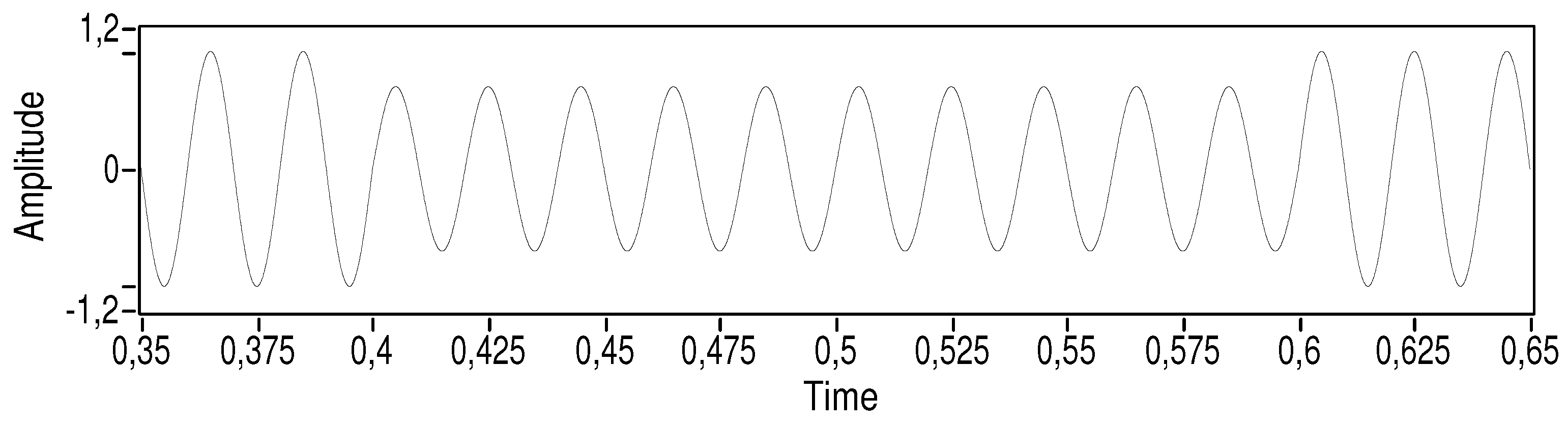
Figure 2. Sag. Time series of a sag with a depth of 30% and a duration of 10 cycles.

Figure 2. Sag. Time series of a sag with a depth of 30% and a duration of 10 cycles.

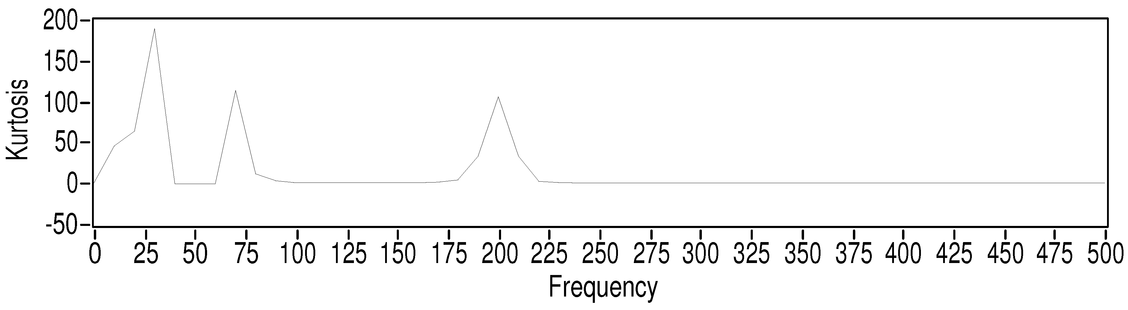
Figure 3. SK analysis over a sag. SK analysis shown from 0 to 500 Hz of a sag with Gaussian additive noise with σ = 0.05.

Figure 3. SK analysis over a sag. SK analysis shown from 0 to 500 Hz of a sag with Gaussian additive noise with σ = 0.05.

As said above, a sag is a reduction in the amplitude of the base waveform. In this experiment, the amplitude has been reduced by 30%, with crisp transitions.

In relation to the SK analysis, there are some changes. First, the vertical axis limits have been changed. The graph in Figure 1 shows the kurtosis values from −1.1 to 0.4. Now, it spreads from −15 to 190.

From 100 Hz onwards, the kurtosis response is constant, close to zero. If a zoom is made over this area, the same response is observed. However, with this vertical scale, it seems a constant value. The main change occurs in frequencies under 100 Hz. Two peaks appear, one of them before 50 Hz and the other one after this frequency component. This separation is occasioned by the same −1 peak at 50 Hz, seen in the previous analysis. As an important length is computed, even with the momentary change of amplitude, 50 Hz is still considered as a constant amplitude. That is represented with the −1 value at 50 Hz. Here, the $-1$ kurtosis value could not be seen due to the vertical scale, but it shows exactly the same value as in the healthy signal. When the amplitude of a single frequency changes suddenly, the surrounding frequencies are affected, as well. That is the situation now. A kurtosis increase for frequencies around 50 Hz means an increase in the variability of these components. They do not reach important amplitudes, however, as they do not show any amplitude before; this means important amplitude variations.

Different sag conditions have been tested in the next experiment, keeping the noise contamination constant in σ = 0.05. Depths from 10 to 90% are settled, considering durations from 5 to 20 cycles. In each signal, kurtosis values for frequencies of 30, 50, 70, 100 and 150 Hz are taken. These frequencies are related to the first peak, the base frequency, the second peak, a near frequency in which the system is slightly altered and a far frequency in which the system is almost unaffected. All information related to those experiments is shown in the Table 2.

Table 2. SK analysis results for sag disturbance with different depths and lengths.

Sag deep	Sag length	Kurtosis
(%)	(Cycles)	30 Hz	50 Hz	70 Hz	100 Hz	150 Hz
10	5	8794	−0.999	4842	0.067	0.126
10	10	9044	-0.999	2,643	−0.053	0.074
10	20	8175	−0.999	2592	−0.047	0.084
20	5	81,769	−0.999	33,701	0.051	0.127
20	10	81,857	−0.999	35,095	−0.005	0.077
20	20	77,130	−0.998	27,154	0.193	0.080
30	5	173,911	−0.999	98,029	1066	0.146
30	10	181,324	−0.999	102,501	1099	0.088
30	20	178,341	−0.998	95,583	1160	0.084
40	5	256,598	−0.999	174,311	2660	0.185
40	10	261,075	−0.998	172,657	1127	0.242
40	20	260,819	−0.996	168,985	2234	0.108
50	5	319,816	−0.999	233,250	6121	0.199
50	10	329,233	−0.997	237,407	3534	0.208
50	20	323,410	−0.995	244,310	5246	0.151
60	5	361,178	−0.998	289,918	11,350	0.305
60	10	368,614	−0.997	288,906	9536	0.237
60	20	366,564	−0.994	290,237	11,325	0.242
70	5	392,615	−0.998	329,945	16,659	0.334
70	10	398,564	−0.996	326,260	16,300	1,121
70	20	396,867	−0.993	327,962	17,368	0.366
80	5	415,655	−0.998	360,687	29,481	0.828
80	10	418,429	−0.996	357,976	27,213	0.890
80	20	418,173	−0.992	359,114	26,520	0.769
90	5	431,010	−0.998	386,573	38,483	1488
90	10	433,368	−0.996	384,002	42,927	1236
90	20	433,365	−0.992	383,941	40,564	0.830

Table 2. SK analysis results for sag disturbance with different depths and lengths.

Sag deep	Sag length	Kurtosis
(%)	(Cycles)	30 Hz	50 Hz	70 Hz	100 Hz	150 Hz
10	5	8794	−0.999	4842	0.067	0.126
10	10	9044	-0.999	2,643	−0.053	0.074
10	20	8175	−0.999	2592	−0.047	0.084
20	5	81,769	−0.999	33,701	0.051	0.127
20	10	81,857	−0.999	35,095	−0.005	0.077
20	20	77,130	−0.998	27,154	0.193	0.080
30	5	173,911	−0.999	98,029	1066	0.146
30	10	181,324	−0.999	102,501	1099	0.088
30	20	178,341	−0.998	95,583	1160	0.084
40	5	256,598	−0.999	174,311	2660	0.185
40	10	261,075	−0.998	172,657	1127	0.242
40	20	260,819	−0.996	168,985	2234	0.108
50	5	319,816	−0.999	233,250	6121	0.199
50	10	329,233	−0.997	237,407	3534	0.208
50	20	323,410	−0.995	244,310	5246	0.151
60	5	361,178	−0.998	289,918	11,350	0.305
60	10	368,614	−0.997	288,906	9536	0.237
60	20	366,564	−0.994	290,237	11,325	0.242
70	5	392,615	−0.998	329,945	16,659	0.334
70	10	398,564	−0.996	326,260	16,300	1,121
70	20	396,867	−0.993	327,962	17,368	0.366
80	5	415,655	−0.998	360,687	29,481	0.828
80	10	418,429	−0.996	357,976	27,213	0.890
80	20	418,173	−0.992	359,114	26,520	0.769
90	5	431,010	−0.998	386,573	38,483	1488
90	10	433,368	−0.996	384,002	42,927	1236
90	20	433,365	−0.992	383,941	40,564	0.830

As indicated above, at 50 Hz, the peaks could be considered −1, even in the higher depth and length conditions. Values in this table are truncated, not rounded.

The durations of the disturbances have no effect on the kurtosis values, keeping the same value for each depth. In relation to the depth, a higher one involves a higher alteration of the waveform. SK detects frequency variability, showing higher values of kurtosis as sag depth increases.

In Table 2 and in Figure 3, it is seen that the 30-Hz frequency peak has a kurtosis value higher than the peak at 70 Hz. In a visual examination of all experiments, 100 Hz seems not to be altered by the sag disturbance. However, a detailed analysis reveals that the kurtosis value is increased when peaks reach important values. Nevertheless, the value associated with 150 Hz is hardly altered, even in the higher depth and length conditions.

Up to now, the base condition of a healthy signal and a sag disturbance alone has been intensely studied. Sag will be coupled to some disturbances. SK analysis will be studied in all of the situations, searching the characteristics of all disturbances introduced, with the goal of differentiating all of them. In the rest of the experiments, a depth of 30% and a length of 10 cycles have been selected.

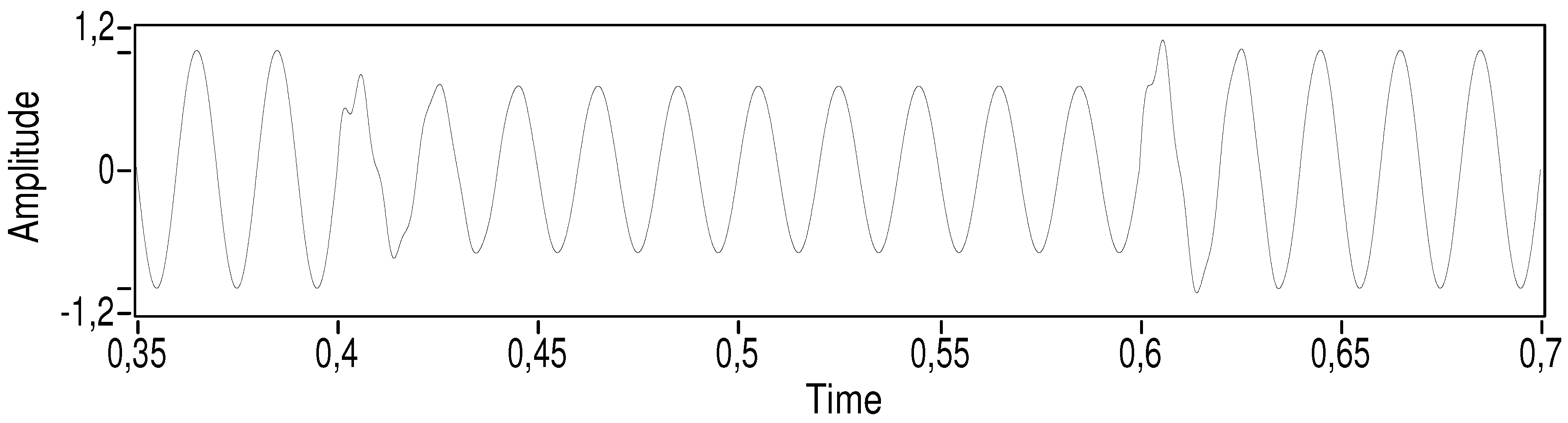
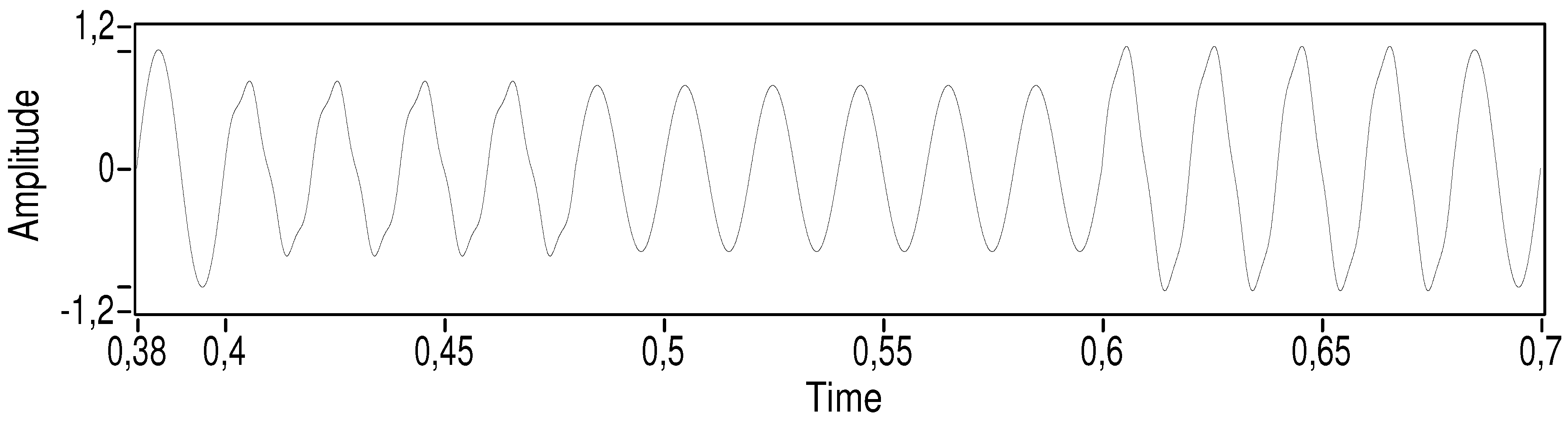
Then, the oscillatory transient will be coupled to the sag. It consists of oscillations around the normal waveform value, with a crisp start and the exponential decay of its amplitude. The signal shown in Figure 4 is composed of the sag indicated before and the oscillatory transient with oscillations of 200 Hz, a duration of four cycles of the power waveform and an initial amplitude of 0.2. It has one oscillatory transient at the sag start and another at the sag end. As in previous graphs, this is shown without noise, in order to observe the disturbance better. In Figure 5, the SK analysis of the coupled signal is shown.

Figure 4. Sag with a coupled oscillatory transient. Time series of a sag with a depth of 30% and a duration of 10 cycles, with an oscillatory transient with a maximum amplitude of a 0.2, a duration of four cycles of the power signal and a frequency of 200 Hz.

Figure 4. Sag with a coupled oscillatory transient. Time series of a sag with a depth of 30% and a duration of 10 cycles, with an oscillatory transient with a maximum amplitude of a 0.2, a duration of four cycles of the power signal and a frequency of 200 Hz.

Figure 5. SK analysis over a sag with a coupled oscillatory transient. SK results shown from 0 to 500 Hz of a sag with an coupled oscillatory transient, with Gaussian additive noise with σ = 0.05.

Figure 5. SK analysis over a sag with a coupled oscillatory transient. SK results shown from 0 to 500 Hz of a sag with an coupled oscillatory transient, with Gaussian additive noise with σ = 0.05.

The main frequency introduced with the oscillatory transient is 200 Hz. As mentioned above, the sags do not alter the frequency over 150 Hz. At first glance, a new element could be seen. In the zone of the graph corresponding to lower frequencies, the same peaks as in the sag situation could be seen. Thus, the sags are detected the same as if this were the only disturbance. However, another peak appears around 200 Hz, which is the oscillatory frequency. This last peak is associated with the oscillatory transient.

As in the sag case, an oscillatory transient supposes an amplitude variation. However, on the contrary, it does not show a constant amplitude during all of the analyzed vectors, so it does not have a −1 value in the central frequency. The sudden start in an oscillatory transient creates an increment in the variability of oscillation frequency. In addition, the transient amplitude is continuously decreasing, which increases the variability of the oscillation frequency more. All of this affects the surrounding frequencies, increasing their variability, as well. The result of all of this is the peak shown in the graph, with a maximum value in the central frequency and a soft decreasing of the kurtosis value as the frequency moves away from 200 Hz, symmetrically in both directions.

Some oscillatory transient conditions are considered, keeping the same sag conditions as indicated before. The oscillatory transient amplitudes taken are from 0.15 to 0.3, and the lengths considered for each amplitude are from two to 10 power signal cycles. As symmetrical peak is returned; only the information of the half peak is taken, being similar on the other side. The kurtosis values for frequencies of 200, 210, 220 and 230 Hz have been taken, and the peak width is measured with the number of points around 200 Hz that have kurtosis values over three. This can be seen in Table 3.

Table 3. SK analysis results for a sag with an oscillatory transient coupled with different conditions.

Transient	Transient	Kurtosis value				Peak
amplitude	length	200 Hz	210 Hz	220 Hz	230 Hz	width
0.15	2	4026	3654	1519	0.446	4
0.15	4	28,877	20,731	6484	1958	6
0.15	6	58,321	40,097	12,979	2461	6
0.15	10	80,057	50,000	10,989	2050	6
0.20	2	12,743	10,804	4,665	1882	6
0.20	4	62,293	49,007	12,880	3077	7
0.20	6	93,304	71,551	22,576	3445	7
0.20	10	118,725	91,339	25,939	4212	8
0.25	2	32,125	23,639	10,084	5794	11
0.25	4	99,072	82,614	35,334	10,221	11
0.25	6	140,299	117,120	45,022	11,404	12
0.25	10	150,465	132,738	56,852	11,749	13
0.30	2	54,755	39,571	19,989	9493	13
0.30	4	148,846	117,608	53,017	17,717	13
0.30	6	167,414	152,665	78,887	23,714	14
0.30	10	169,960	166,178	83,782	23,326	13

Table 3. SK analysis results for a sag with an oscillatory transient coupled with different conditions.

Transient	Transient	Kurtosis value				Peak
amplitude	length	200 Hz	210 Hz	220 Hz	230 Hz	width
0.15	2	4026	3654	1519	0.446	4
0.15	4	28,877	20,731	6484	1958	6
0.15	6	58,321	40,097	12,979	2461	6
0.15	10	80,057	50,000	10,989	2050	6
0.20	2	12,743	10,804	4,665	1882	6
0.20	4	62,293	49,007	12,880	3077	7
0.20	6	93,304	71,551	22,576	3445	7
0.20	10	118,725	91,339	25,939	4212	8
0.25	2	32,125	23,639	10,084	5794	11
0.25	4	99,072	82,614	35,334	10,221	11
0.25	6	140,299	117,120	45,022	11,404	12
0.25	10	150,465	132,738	56,852	11,749	13
0.30	2	54,755	39,571	19,989	9493	13
0.30	4	148,846	117,608	53,017	17,717	13
0.30	6	167,414	152,665	78,887	23,714	14
0.30	10	169,960	166,178	83,782	23,326	13

It is worth remarking about the following issues. Firstly, the length of two cycles reduces the kurtosis value in the oscillation frequency, for all amplitude situations. Simulation creates a sinusoidal wave with the desired length and applies an exponential decrease in the transient amplitude, which ends in zero. The shorter the transients were, the more the amplitude of the first cycle would be reduced. This reduces the initial change of the amplitude. Moreover, the variability is related to the change of amplitude during the transient, and as it has a lower extension, the variability is reduced, as well.

This trend continues as length increases. All kurtosis values are higher as the lengths of transients increase. This could be observed in any frequency for any amplitude considered in the table.

As indicated before, the frequencies selected in the table are related to the half peak. The alteration of SK is symmetrical, as can be seen in Figure 5. As the transient amplitude increases, the peak turns softer. This means a higher variation as the frequency moves away from the central one. For the 0.3 amplitude and a 10-cycle length, the kurtosis associated with 200 and 210 Hz is almost the same, and the next frequency shows half value of them. However, for the same length, taking an amplitude of 0.2, a change from 200 to 210 Hz supposes a loss of 23%, and in the next step, it losses 71%. Higher variations, as seen for the second one, mean a pointier peak. Lower kurtosis variations among near frequencies, as in the first one, create a softer peak, with a rounder shape.

In addition, the higher amplitude means a higher variability itself. At the starting moment, it creates a bigger step, and then, during the exponential decay, a bigger change is observed. Taking the same two situations, with an amplitude of 0.3 and a length of 10 cycles, the maximum value returned is 169.96. With the same length, and for an amplitude of 0.2, a peak with a maximum of 118.72 is originated.

The last column shows the width of the peaks, taking a threshold of three. An increase in the length multiplies the kurtosis value associated with each frequency. As frequencies near the end of each peak have very low values, multiplying them does not change the situation very much. This could be observed by the fact that almost the same length is indicated for each amplitude. On the other hand, as the transient amplitude increases, the kurtosis value is incremented, increasing at the same time the peak widths and turning them softer.

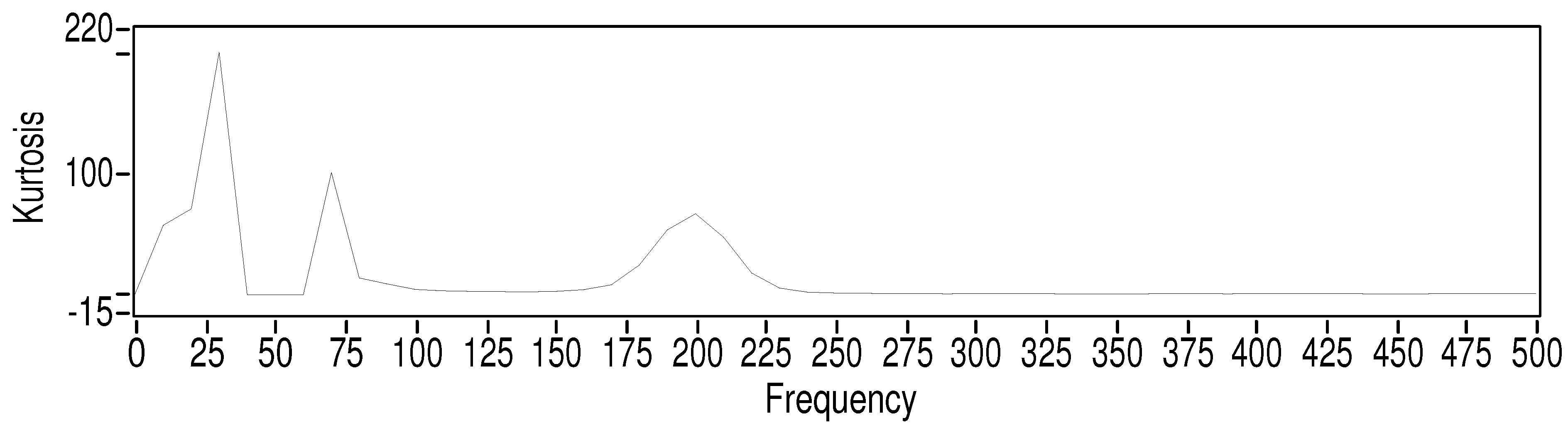
The last disturbance considered is the harmonic distortion at the sag start and end. The harmonic selected is the fourth one, which implies a frequency of 200 Hz. This one has been used in order to introduce the same frequency as in the previous test. In the oscillatory transient situation, oscillations starts with a high amplitude, and this decays in an exponential way. On the other hand, the harmonics take the same amplitude during all of the disturbed segment. In Figure 6, the signals with harmonic distortion are shown, and the SK analysis is shown in Figure 7 from 0 to 500 Hz.

The conditions for the sag are the same as in the previous experiments. The same frequency has been introduced; any difference observed in relation to the oscillatory transient are due to harmonic distortion. The oscillatory transient introduced in Figure 4 starts with a high alteration; however, the signal recovers its normal state very quickly. On the other hand, in Figure 6, changes in the signal are at the same level for all of the disturbed segment.

In Figure 7, the same response for frequencies under 100 Hz as in Figure 5 can be seen. This is related to the sag: as the same conditions have been considered, its response remains equal, as well. There is another peak around 200 Hz, in the same position as in the previous experiment. However, the peak’s shape is different. Now, it takes a shorter extension and reaches a higher kurtosis value, resulting in a pointier peak than in the previous situation.

Figure 6. Sag with harmonic distortion. Time series of a sag with a depth of 30% and a duration of 10 cycles with harmonic distortion with an amplitude of a 0.07 and a duration of four cycles of the power signal. The fourth harmonic has been selected (200 Hz).

Figure 6. Sag with harmonic distortion. Time series of a sag with a depth of 30% and a duration of 10 cycles with harmonic distortion with an amplitude of a 0.07 and a duration of four cycles of the power signal. The fourth harmonic has been selected (200 Hz).

Figure 7. Sag analysis with harmonic distortion. SK results shown from 0 to 500 Hz of a sag with harmonic distortion, with Gaussian additive noise with σ = 0.05.

Figure 7. Sag analysis with harmonic distortion. SK results shown from 0 to 500 Hz of a sag with harmonic distortion, with Gaussian additive noise with σ = 0.05.

As in the oscillatory transient experiment, some harmonic disturbance conditions will be tested, keeping the sag conditions and the harmonic distortion frequency equal. Harmonic distortion amplitudes have been taken from 0.07 to 0.20, using lengths from one to four cycles of the base waveform. The results of these experiments are shown in Table 4. As in the oscillatory transient situation, the kurtosis value related to each signal has been taken for frequencies of 200, 210, 220 and 230 Hz, and the peak widths have been measured as the number of points with a kurtosis value over three around 200 Hz.

In this experiment, lower extensions and amplitudes have been considered. Even with that, higher kurtosis values are obtained.

Examining Figure 6, the harmonic distortion peak looks pointier than the one related to the oscillatory transient, shown in Figure 4. Comparing the conditions shown in the figures, for the same length, four cycles of the base waveform, harmonic distortion with an amplitude 0.07 creates a three-point peak with a maximum value of 104, and an oscillatory transient, with an amplitude of 0.20, creates a seven-point peak with a maximum value of 62. The peak related to harmonic distortion shows a higher kurtosis value and a lower width than that related to the oscillatory transient.

If the same conditions are used for harmonic distortion and the oscillatory transient, for example an amplitude of 0.20 and a length of four cycles of the base waveform, different results are obtained. Harmonic distortion gives a peak with a maximum value of 261 and a width of nine, and the oscillatory transient returns a peak with a maximum value of 62 and a width of seven. Now, the peak related to harmonic distortion is wider; however, if the ratio between the maximum value and the width is shown, the harmonic distortion has 260/9 = 28.9 and the oscillatory transient 62/7 = 8.8. This means that the harmonic peak is taller in relation to its width than the one related to the oscillatory transient.

Table 4. SK analysis results for sag with harmonic distortion coupled with different conditions.

Harmonics	Transient	Kurtosis value				Peak
amplitude	length	200 Hz	210 Hz	220 Hz	230 Hz	width
0.07	1	10,048	5804	3028	0.549	5
0.07	2	28,624	18,553	2112	0.156	4
0.07	3	58,138	25,196	2011	0.200	4
0.07	4	104,395	34,220	1069	0.209	3
0.10	1	32,189	25,505	11,373	2150	6
0.10	2	64,873	44,329	6894	0.540	5
0.10	3	116,762	68,756	6654	0.571	5
0.10	4	169,964	72,610	4926	0.637	5
0.15	1	84,983	72,386	41,950	9014	9
0.15	2	127,734	89,248	20,804	1935	7
0.15	3	174,153	126,729	23,235	2674	6
0.15	4	236,331	129,797	13,634	1399	5
0.20	1	149,340	135,240	84,174	27,454	8
0.20	2	178,761	133,981	49,134	7189	9
0.20	3	207,419	164,963	45,999	6692	8
0.20	4	261,294	166,906	41,016	5087	9

Table 4. SK analysis results for sag with harmonic distortion coupled with different conditions.

Harmonics	Transient	Kurtosis value				Peak
amplitude	length	200 Hz	210 Hz	220 Hz	230 Hz	width
0.07	1	10,048	5804	3028	0.549	5
0.07	2	28,624	18,553	2112	0.156	4
0.07	3	58,138	25,196	2011	0.200	4
0.07	4	104,395	34,220	1069	0.209	3
0.10	1	32,189	25,505	11,373	2150	6
0.10	2	64,873	44,329	6894	0.540	5
0.10	3	116,762	68,756	6654	0.571	5
0.10	4	169,964	72,610	4926	0.637	5
0.15	1	84,983	72,386	41,950	9014	9
0.15	2	127,734	89,248	20,804	1935	7
0.15	3	174,153	126,729	23,235	2674	6
0.15	4	236,331	129,797	13,634	1399	5
0.20	1	149,340	135,240	84,174	27,454	8
0.20	2	178,761	133,981	49,134	7189	9
0.20	3	207,419	164,963	45,999	6692	8
0.20	4	261,294	166,906	41,016	5087	9

As indicated before, with the same conditions, the harmonic distortion generates kurtosis responses higher than the oscillatory transients. Taking the conditions of an amplitude of 0.20 and a duration of two cycles, the maximum kurtosis values are 12.7 for the oscillatory transient and 178.7 for the harmonic distortion. This difference is accentuated for a duration for four cycles and the same amplitude, reaching values of 62.3 for the oscillatory transient and 261.3 for the harmonic distortion. If the same maximum value is searched, an amplitude of 0.07 and a duration of three cycles must be used for harmonic distortion, obtaining a value of 58.13, and an amplitude of 0.15 with a duration of six cycles for the oscillatory transient, obtaining a value of 58.32.

As said before, the peaks associated with harmonic distortion are sharper than the ones related to the oscillatory transients, and now, this will be detected over the kurtosis evolution. First, the kurtosis change from the peak central frequency (200 Hz) to the next one (210 Hz) will be examined, for common conditions. These are amplitudes of 0.15 and 0.20 and durations of two and four base signal cycles. In these conditions, the change rates are from 9% to 30% for oscillatory transients and from 25% to 45% for harmonic distortion. If all simulations are examined, variation rates of 2% and 37% are obtained for oscillatory transients, and for harmonics distortion, these take values from 9% to 67%. Taking common conditions or taking all simulations, a higher variation could be observed for harmonic distortion. This higher change implies a crisper peak.

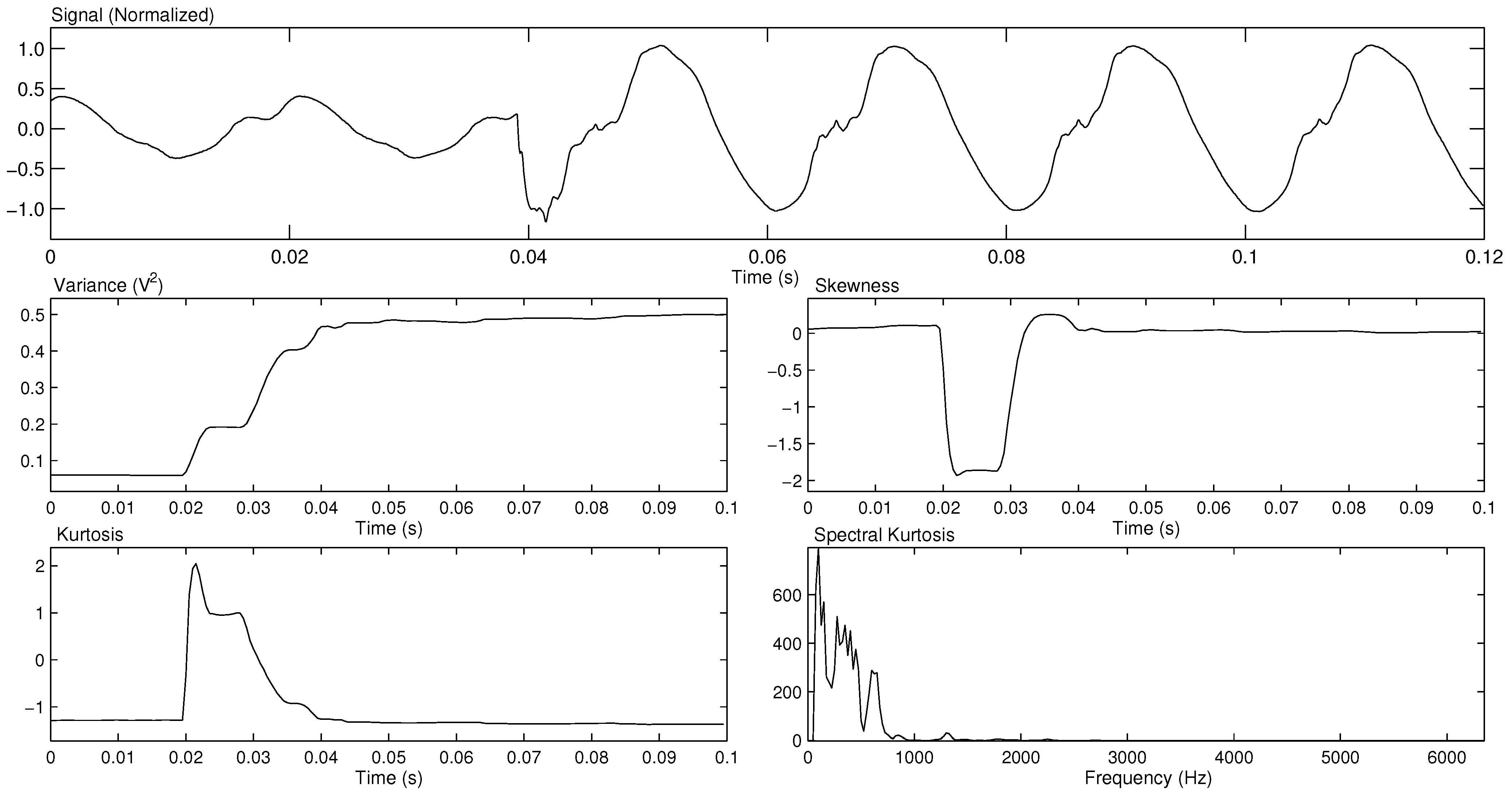
With the goal of considering a real-life situation, we have introduced Figure 8, where a sag is accompanied by a severe harmonic distortion (the same as in Figure 8) in a Gaussian additive noise floor with σ=0.5. In this case, the measurement bandwidth is wider, taking the whole profit of the data acquisition equipment, connected via a differential probe to the phase voltage A-B. The complete analysis is also shown, where the time domain variance (power variations), skewness (indicator of the waveform symmetry) and the kurtosis (peakedness of the time domain signal) are also presented. The peaks in the SK graph are the same as those in Figure 7. In fact, the amplitude transition is reflected as a spectral leakage around the harmonics. Indeed, the y-axis in the SK graphs accounts for variability, as the kurtosis is an estimator of the peakedness of the probability density function associated with the measurement time series.

Figure 8. SK analysis over a sag with harmonic distortion, with Gaussian additive noise with $\sigma =0.05$. If harmonics at 25 and 75 Hz are present and there is no sag, two “clean” spectral lines would appear. In the case of a hybrid event, the SK outlines the spectral leakage around the harmonic frequencies.

Figure 8. SK analysis over a sag with harmonic distortion, with Gaussian additive noise with $\sigma =0.05$. If harmonics at 25 and 75 Hz are present and there is no sag, two “clean” spectral lines would appear. In the case of a hybrid event, the SK outlines the spectral leakage around the harmonic frequencies.

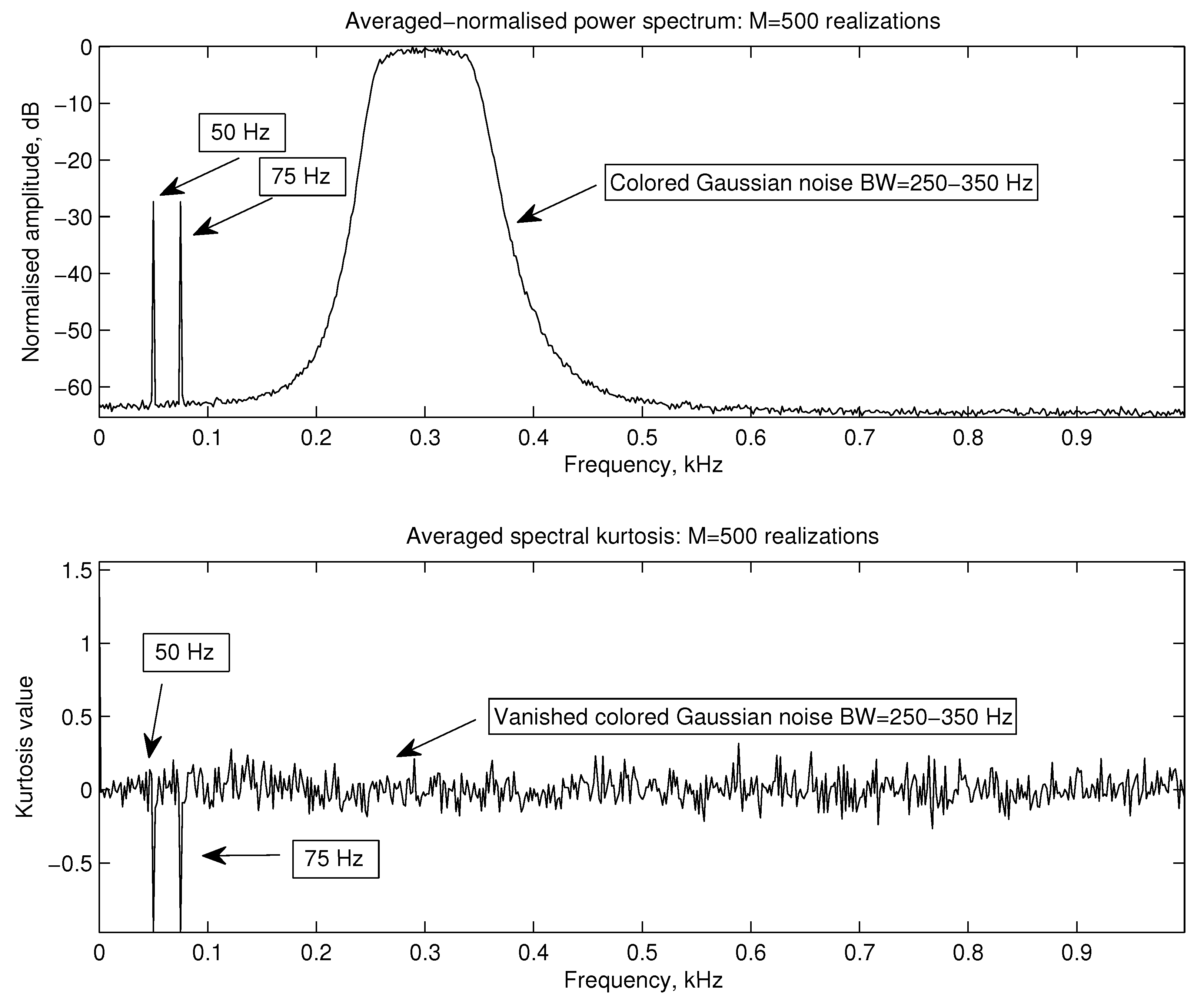
Finally, and with the two-fold purpose of illustrating harmonic detection and noise rejection at the same time, two pure harmonics (at 50 and 75 Hz) have been contaminated by colored Gaussian noise (σ = 0.05, bandwidth: 250 to 350 Hz). The effect is the clear distinction of the two spectral lines along with the noise vanishing. In Figure 9, the spectral lines are outlined both in the second and in the fourth-order domain (SK); in the latter, noise is completely rejected, as expected by a higher-order spectrum.

Figure 9. Harmonics’ discrimination and noise rejection. Harmonics at 50 and 75 Hz have been mixed with colored Gaussian noise (σ = 0.05, bandwidth: 250 to 350 Hz).

Figure 9. Harmonics’ discrimination and noise rejection. Harmonics at 50 and 75 Hz have been mixed with colored Gaussian noise (σ = 0.05, bandwidth: 250 to 350 Hz).

4. Conclusions

This paper shows that the SK has good noise resistance and is a robust spectral analysis tool, returning a similar response with different noise contamination levels (uniform and Gaussian noise produce the same results). As a variability analysis tool, associating the peakedness of the probability density function, and in the frame of PQ analysis, different sag depths have returned different kurtosis maximum values, but always with the same shape, showing the SK normal value at 150 Hz. The sag length has no effect on the kurtosis response, showing similar values for each sag depth.

In the coupled disturbances study, sag conditions have been set constant in order to obtain similar test conditions. A frequency of 200 Hz has been introduced with oscillatory transients and harmonic distortion, returning a peak centered at the same position. Peaks related to these show a maximum width of 140 Hz, which means a range from 130 to 270 Hz. In the considered sag conditions, the maximum kurtosis value is 0.8 at 130 Hz, with an average kurtosis value of 0.05. That confirms that there is no interference from the sag SK response for the oscillatory transient and harmonic disturbance SK response.

Oscillatory transients show an exponential amplitude decay, so the alteration of the base wave is lower than in harmonic distortion, because this second situation keeps its amplitude constant. In addition, the oscillatory transient has one hard transition, at its start, because of its end amplitude being zero. On the other hand, harmonic disturbance have two hard transitions, one at its start and one at its end. All of these create higher values in harmonic disturbance situations, with even higher impact on the central frequency, for the same amplitude and length conditions. In addition, crisper peaks are obtained in harmonic distortion, due to a higher impact over the central frequency than in the oscillatory transient situation, in which adjacent frequencies are more affected. Taking all of this into consideration, when a symmetrical peak appears in the SK response, wide and soft ones are related to oscillatory transients and narrow and crisp ones to harmonic distortion.

As a final remark, the performance of the SK over hybrid (mixed) PQ events is promising, and it has been proven over a set of synthetics. The next step will focus the implementation on an autonomous measurement system, which requires adapting the measurement requirements to norms or the International Electrotechnical Commission (IEC). Compliance with the standards [27,28] that define the conditions for data acquisition in harmonic measurements for power supply systems implies the use of a basic acquisition window corresponding to a time period of Δt=200 ms. Sampling frequency and the rest of the parameters have to be adapted to these requirements.