Assessment of the Wave Energy in the Black Sea Based on a 15-Year Hindcast with Data Assimilation

Abstract

The principal target of the present work is to assess the wave energy potential in the Black Sea, identifying also some relevant energetic features and possible patterns. A wave prediction system based on the Simulating Waves Nearshore model (SWAN) has been implemented and intensively tested in the entire sea basin. Moreover, considering an optimal interpolation technique, an assimilation scheme of the satellite data has been developed, leading to a visible improvement of the wave model predictions in terms of significant wave heights and, consequently, also in terms of wave power. Using this wave prediction system with data assimilation, simulations have been performed for a 15-year period (1999–2013). Considering the results of this 15-year wave hindcast, an analysis of the wave energy conditions in the basin of the Black Sea has been carried out. This provided a more comprehensive picture concerning the wave energy patterns in the coastal environment of the Black Sea focused on the average wave conditions that might be expected in this sea. Following the results presented, it can be concluded that the wave energy extraction in the Black Sea can become an issue of interest, especially from the perspective of the hybrid solutions.

1. Introduction

The Black Sea is an enclosed and marginal sea basin, located in the Southeastern part of Europe. It drains through the Mediterranean Sea into the Atlantic Ocean, via the Aegean Sea and various straits. These are Bosphorus that connects the Black Sea to the Sea of Marmara, and Dardanelles connecting the Sea of Marmara to the Aegean Sea, which is in fact a region of the Mediterranean Sea. This water body separates Eastern Europe and Western Asia. The Black Sea is also connected to the Sea of Azov by the Strait of Kerch. Without including the Sea of Azov, the Black Sea has an area of 436,400 km², a volume of 547,000 km³ and a maximum depth of 2212 m (Figure 1).

Figure 1. The SWAN computational domain considered for performing model simulations in the Black Sea. In the background the bathymetric map is illustrated while in the foreground the wave vectors corresponding to one of the most relevant wave propagation patterns are presented. The position of the Gloria drilling unit that operates in the Romanian nearshore is also indicated and the position of the reference points considered for the local analyses.

Figure 1. The SWAN computational domain considered for performing model simulations in the Black Sea. In the background the bathymetric map is illustrated while in the foreground the wave vectors corresponding to one of the most relevant wave propagation patterns are presented. The position of the Gloria drilling unit that operates in the Romanian nearshore is also indicated and the position of the reference points considered for the local analyses.

Due to the fact that the Black Sea receives river waters from the large Eurasian fluvial systems in its northern part, its water balance is positive. This means a net outflow of water into the Aegean Sea of about 300 km³ per year. On the other hand, the more saline and warmer water from the Mediterranean Sea flows into the Black Sea as part of a two-way hydrological exchange. The water outflowing from the Black Sea is less saline and cooler and floats over the water inflowing from the Mediterranean Sea. The sea basin is divided into two sub-basins. The Black Sea’s circulation patterns are primarily controlled by the fluvial inputs and the basin topography. The mean surface circulation is cyclonic and the water circulates around the Black Sea in a basin-wide pattern, known as the Rim Current. This usually has a maximum velocity of about 0.5–1.0 m/s. Two smaller cyclonic gyres operate, occupying the eastern and western sectors of the basin. These are well-organized systems in the winter but dissipate into a series of interconnected eddies in the summer and autumn. Moreover, outside of the Rim Current, numerous other quasi-permanent coastal eddies are formed as a result of upwelling around the coastal apron and “wind curl” mechanisms. The intra-annual strength of these features is controlled by seasonal atmospheric and fluvial variations [1,2,3,4].

Due to its geographical position, the Black Sea climate is influenced by air masses coming from various directions. The marine tropical air masses occur due to the southwest winds from the Mediterranean basin, while during the winter the presence of the polar air masses coming from north and northeast lead to low temperatures and frequent storms in the basin [5,6]. In this period, the sea forms an elliptical depression east–west, which is constrained by the Caucasus Mountains in the east and by the Pontic Mountains in the south. A comprehensive picture of the wind conditions in the Black Sea is presented in [7,8] and according also to these sources the most energetic part of the Black Sea is its western side. The longest east–west sea extent is about 1175 km and, although this fetch is considerably smaller than in open-ocean, the strong winter winds can generate waves in this environment that might become comparable in magnitude with those from the ocean [9].

On the other hand, due to the high demand for lower-carbon energy systems that should contribute to the decarbonization of the energy sector [10,11], since greenhouse gas emissions are widely recognized factors in the climate changes, the importance of extracting the renewable energy from the marine environment become an issue of increasing importance. From this perspective, and taking into account the fact that the renewable energy extraction in the countries located in the western side of the Black Sea is presently limited to several onshore wind projects and water dams, the objective of the present work is to provide a more comprehensive picture of the wave energy potential in the basin of the Black Sea. This starts from the output provided by some previous studies [12,13] and considers the results of a 15-year wave hindcast (1999–2013) performed with numerical wave models. Moreover, in order to increase the reliability of the model outputs, an assimilation scheme of the satellite data has been developed and implemented for the entire 15-year period.

2. Wave Modelling

2.1. Theoretical Background of the Spectral Wave Models

The model considered for performing simulations in the basin of the Black Sea is Simulating Waves Nearshore (SWAN) [14]. This is one of the state-of-the-art wave models based on the spectrum concept. Such models integrate the energy balance Equation (1) describing the variation of the wave energy spectrum in the fifth dimensions, represented by time, geographic, and spectral spaces (the spectral space is defined by the relative frequency $\mathrm{\sigma }$ and the wave direction $\mathrm{\theta }$):

$$\frac{\partial N}{\partial t}+\frac{\partial }{\partial \mathrm{\lambda }}{c}_{\mathrm{\lambda }}N+\frac{1}{\cos \mathrm{\phi }}\frac{\partial }{\partial \mathrm{\phi }}{c}_{\mathrm{\phi }}N\cos \mathrm{\phi }+\frac{\partial }{\partial \mathrm{\sigma }}{c}_{\mathrm{\sigma }}N+\frac{\partial }{\partial \mathrm{\theta }}{c}_{\mathrm{\theta }}N=\frac{S}{\mathrm{\sigma }}$$

(1)

where N is the action density spectrum defined as the ratio between the energy density and relative frequency, $c_{\mathrm{\lambda }}$ and $c_{\mathrm{\phi }}$ are the components of the relative group velocity ${\overrightarrow{c}}_g$ for the geographical space (${\overrightarrow{c}}_g=\partial \mathrm{\sigma }/\partial \overrightarrow{k}$, with k the wave number), $c_{\mathrm{\sigma }}=\dot{\mathrm{\sigma }}$ and $c_{\mathrm{\theta }}=\dot{\mathrm{\theta }}$ are the propagation velocities in the spectral space and t is the time. In the right hand side of the action balance equation, and S is the total source expressed in terms of energy density.

In the expression of the total source term three components are significant in deep water, and they correspond to the atmospheric input (S_in), whitecapping dissipation (S_dis), and nonlinear quadruplet interactions (S_nl), respectively. Additional source terms are considered in shallow water (S_sw) to account for the finite depth effects. Hence the total source becomes:

$$S=S_{in}+S_{dis}+S_{nl}+S_{sw}$$

(2)

If the medium itself is moving with the velocity $\overrightarrow{U}$ the frequency of the wave passing a field point is shifted due to the Doppler Effect:

$$\mathrm{\omega }=\mathrm{\sigma }+\overrightarrow{k}\cdot \overrightarrow{U}$$

(3)

Usually, the quantity ω is called the observed or absolute frequency while σ is the relative or intrinsic frequency whose functional dependence on k (the wave number in absolute value) is known as the classical dispersion relationship. The actual versions of the spectral wave models deal mainly with the action density spectrum instead of the energy density spectrum. This is because, unlike the energy density, in the presence of the currents the action density is conserved.

In SWAN, the energy transport components over one meter of wave front (in W/m), called also the wave power (P_W) components, are computed with the relationships:

$$\begin{array}{l}{P}_{Wx}=\mathrm{\rho }g{\displaystyle \iint C_{gx}E\left(\mathrm{\sigma },\mathrm{\theta }\right)d\mathrm{\sigma }d\mathrm{\theta }}\\ P_{Wy}=\mathrm{\rho }g{\displaystyle \iint C_{gy}E\left(\mathrm{\sigma },\mathrm{\theta }\right)d\mathrm{\sigma }d\mathrm{\theta }}\end{array}$$

(4)

where E represents the wave energy density spectrum, x, y are the problem coordinate system (for the spherical coordinates, x axis corresponds to the longitude and y axis to the latitude), and C_gx, C_gy are the components of the absolute group velocity ${\overrightarrow{C}}_g$, which is defined as:

$$\frac{d\overrightarrow{x}}{dt}={\overrightarrow{C}}_g=\frac{\partial \mathrm{\omega }}{\partial \overrightarrow{k}}=\frac{\partial \mathrm{\sigma }}{\partial \overrightarrow{k}}+\overrightarrow{U}={\overrightarrow{c}}_g+\overrightarrow{U}$$

(5)

As a result the total wave power becomes:

$$P_W=\sqrt{P_{Wx}^2+P_{Wy}^2}$$

(6)

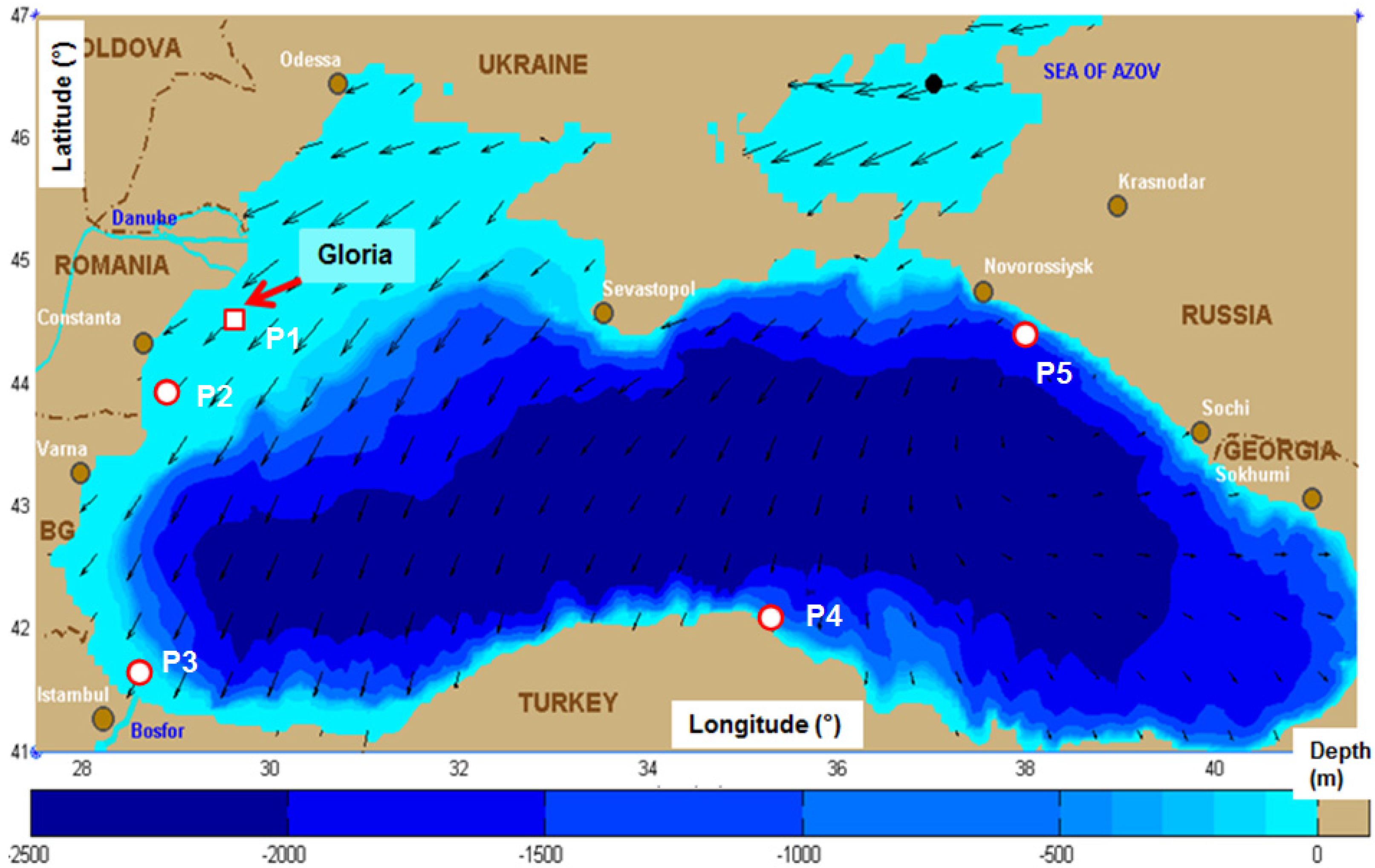
The computational domain defined for the SWAN model simulations in the basin of the Black Sea, also including the Sea of Azov, is presented in Figure 1. The background of the figure illustrates the bathymetry of the sea, while the foreground presents the wave vectors corresponding to one of the most relevant winter time wave propagation patterns. The position of the Gloria drilling platform that operates in the western sector of the Black Sea (44°31′ N, 29°34′ E) at a location where the water depth is about 50 m is indicated in the figure as also the positions of five reference points that were further considered for local analyses.

The system origin corresponds to the lower left corner point and has the coordinates (27.5° E, 41.0° N). The x direction (longitude) extends 14°, while the y direction (latitude) extends 6°. In the geographical space, the computational grid was chosen to coincide with the bathymetric grid and has 176 points in the x direction and 76 points in the y direction. The points are equally spaced with 4.5 min. In the spectral space, 36 directions and 30 frequencies were considered. The frequency range defined is between 0.05 and 1.0 Hz. Some additional details related to the input and to the physical options considered in the SWAN simulations are presented in Table 1.

Table 1. Input and physics considered in the SWAN simulations.

SWAN model	Input/Process
Model version	40.91ABC
Bathymetry	Same resolution as the computational grid
Wind forcing	Wind fields at 10 m from NCEP-CFSR
Physics	Quadruplet nonlinear interactions: fully explicit computation of the nonlinear transfer with DIA (default)
	Exponential growth by wind (Janssen, 1991)
	Whitecapping: Janssen formulation [15]
	Bottom friction: JONSWAP formulation [16]
Computation mode	Non-stationary
Time step	10 min
Numerical scheme	S&L [17]

Table 1. Input and physics considered in the SWAN simulations.

SWAN model	Input/Process
Model version	40.91ABC
Bathymetry	Same resolution as the computational grid
Wind forcing	Wind fields at 10 m from NCEP-CFSR
Physics	Quadruplet nonlinear interactions: fully explicit computation of the nonlinear transfer with DIA (default)
	Exponential growth by wind (Janssen, 1991)
	Whitecapping: Janssen formulation [15]
	Bottom friction: JONSWAP formulation [16]
Computation mode	Non-stationary
Time step	10 min
Numerical scheme	S&L [17]

This wave prediction system was initially validated against in situ measurements, considering for the western side of the Black Sea, especially the measurements performed at the Gloria drilling unit [12], and some validations against remotely-sensed data [18] have been also performed. The results of the above wave prediction system were found, in general, more reliable than those coming from other similar wave modeling systems based on spectral models that were implemented in the basin of the Black Sea [19] and also in line with some other implementations in enclosed, or semi-enclosed, sea environments [20,21,22]. Nevertheless, direct comparisons against in situ measurements, as those performed at the Gloria drilling unit, show that there are still some situations when the accuracy of the wave predictions needs to be substantially improved. That is why, in order to increase the reliability of the wave predictions, some data assimilation (DA) techniques have been developed and associated to the wave modeling system herewith implemented. The methodology considered will be briefly described next.

2.2. Techniques Considered for Assimilation of the Satellite Data

As it is widely known, the main target behind the implementation of the data assimilation techniques is to reduce the systematic errors that may occur in the results provided by the numerical models, taking advantage of the existing measurements. Thus, the basic philosophy of the data assimilation is to combine the complementary information from measurements and the results of the numerical models into an optimal estimate of the geophysical fields of interest [23,24]. The assimilation of the wave data is usually performed in terms of significant wave height (H_s). Measurements of this wave parameter are available locally (generally coming from buoys) and widespread (altimeter data). The sequential methods combine all the observations falling within a particular time window and update the model solution without reference to the model dynamics. The most widely adopted DA schemes are based either on instantaneous sequential procedures, like the optimal interpolation (OI) [25,26], or the successive correction method (SCM) [27]. These methods are attractive, especially due to their lower computational demands, such DA schemes based on OI being widely used in the centers for wave forecasting. In fact, most of the weather prediction centers with wave modelling capabilities are assimilating nowadays altimeter measurements, respectively H_s, using assimilation procedures based on the OI or SCM techniques.

For the current SWAN-based wave modeling system implemented in the basin of the Black Sea, such an algorithm based on OI techniques was considered. This is formulated in the observational space, with the following definitions [25,26]:

$${\mathbf{V}}_a={\mathbf{V}}_b+{\mathbf{C}}_b{\mathbf{F}}^T{[{\mathbf{F}\mathbf{C}}_b{\mathbf{F}}^T+{\mathbf{C}}_o]}^{-1}[\mathbf{O}-F({\mathbf{V}}_b)]$$

(7)

in which O represents the observation vector that contains all the observations available within the time window considered for assimilation (for satellite data, the observations made on the geographical domain defined by the wave model grid are considered); V_b is the background vector (H_s wave model results); V_a is the analysis vector (corrected H_s wave model results); (F,F) represent the forward observational operator and the linear observation operator matrix, respectively, C_o is the observation error covariance; and C_b is the background error covariance.

The Forward Operator represents a method of converting a forecast model variable to an observed variable. In our case, the observations and predicted variables are the same (significant wave height, H_s), and the method reduces to a spatial interpolation of the predictions to the observation locations. The analysis increment is equivalently defined by the relationship ${\mathbf{C}}_b{\mathbf{F}}^T{[{\mathbf{F}\mathbf{C}}_b{\mathbf{F}}^T+{\mathbf{C}}_o]}^{-1}[\mathbf{O}-F({\mathbf{V}}_b)]$ where the quantity ${\mathbf{C}}_b{\mathbf{F}}^T{[{\mathbf{F}\mathbf{C}}_b{\mathbf{F}}^T+{\mathbf{C}}_o]}^{-1}$ represents the weight matrix (which is also commonly called the Kalman gain matrix). The horizontal correlation is computed with the relation:

$$C_h=\exp (-s_h/L_{\max })$$

(8)

in which $s_h$ is the horizontal distance between two locations (observations or observation and a grid point) and L_max is the correlation length of the prediction errors for the wave parameter assimilated [26].

Various studies [28] recommend at about 45° latitude (the Black Sea area being centered on this latitude) a value for the parameter L_max of around 400 km, which represents about 4° degrees. First, this value was used but since, in the Black Sea, the wind-sea waves are dominant, it was considered necessary to also test some lower values for this parameter and to calculate the statistical results obtained after the DA application [29].

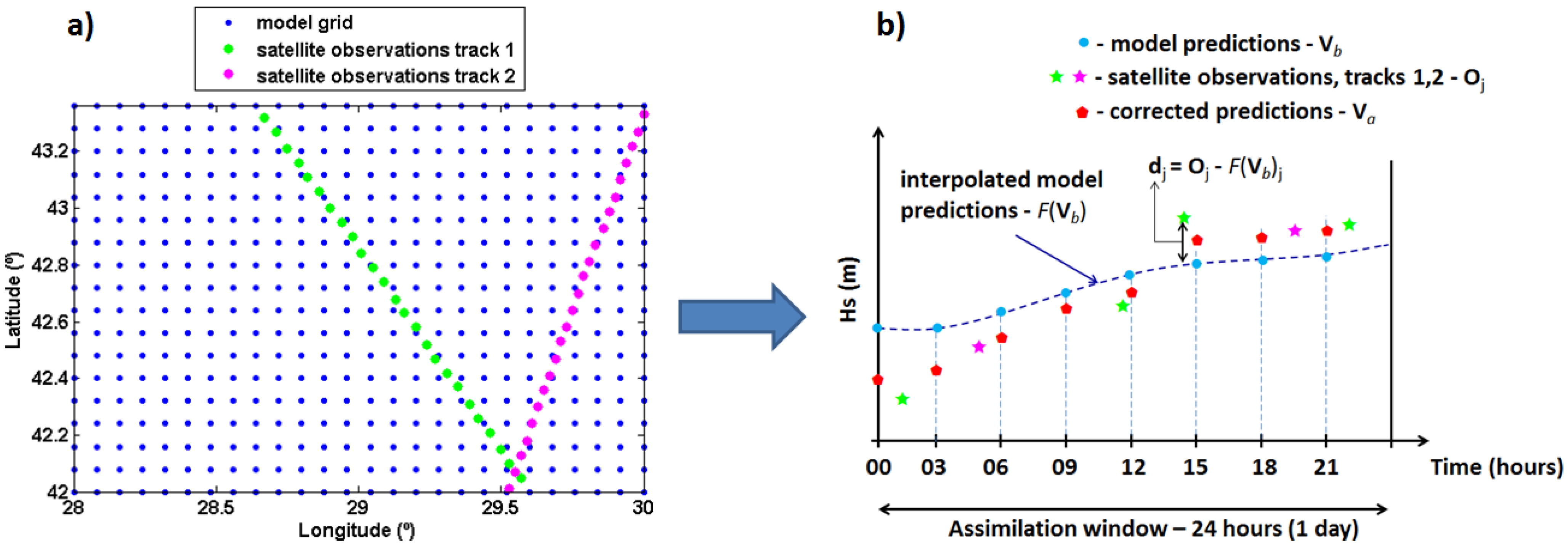
It has to also be highlighted that the effectiveness of the DA techniques are highly dependent on the number of the measured data that are assimilated. For the large areas, the available measurements are only those coming from satellites, which in the recent years have become increasingly more accurate, representing the most viable source for the use in the DA techniques. For the implementation of the DA algorithm in the Black Sea, the measurements from the following satellites have been considered ERS-2, ENVISAT, TOPEX, Poseidon, JASON-1, JASON-2, GEOSAT Follow-On (GFO), Cryosat-2, and SARAL. The assimilation of the altimeter measurements is applied to a window of 24 h (1 day), as shown schematically in Figure 2.

After performing corrections of the significant wave heights in the grid points (G) that are affected by the assimilation process, in order to interact with the wave model, the next step is to transfer this correction in the spectral space. In the SWAN model, the 2D wave energy density spectrum corresponding to a certain simulation ($E_{Gt}^{Sim}$) is discretized in a matrix form as follows:

$$E_{Gt}^{Sim}=\left[E_{Gtnm}^{Sim}\right]$$

(9)

where the index n (n = 1, nf, with nf the number of frequencies) defines the distribution of the wave energy along the frequencies and the index m (m = 1, nd, with nd the number of directions) defines the distribution of the wave energy along the wave directions. Thus, $E_{Gtnm}^{Sim}$ represents the wave energy density (or variance density in m²/Hz/degr) corresponding to the frequency number n and to the direction number m (as defined in the model settings) corresponding to the grid point G and to the simulation performed for the time instant (t). The above spectral matrix can be written in a normalized form as follows:

$$E_{Gt}^{Sim}=E_{Gt\max }^{Sim}\left[E_{GtNnm}^{Sim}\right]$$

(10)

in which $E_{Gt\max }^{Sim}$ is the maximum value of the energy variance and $\left[E_{GtNnm}^{Sim}\right]$ represents the normalized form of the spectral matrix obtained by dividing the elements of the genuine spectral matrix by the maximum value of the energy variance.

Figure 2. (a) Schematic presentation of a computational domain for which wave model predictions exist in the grid points and the satellite tracks crossing the respective area in 24 h; (b) Calculation of the difference d_j between the observation O_j and the prediction interpolated to the observation position F(V_b)_j made at the time of observation, considering the values of the observations recorded in the 1-day assimilation window.

Figure 2. (a) Schematic presentation of a computational domain for which wave model predictions exist in the grid points and the satellite tracks crossing the respective area in 24 h; (b) Calculation of the difference d_j between the observation O_j and the prediction interpolated to the observation position F(V_b)_j made at the time of observation, considering the values of the observations recorded in the 1-day assimilation window.

Finally, in order to propagate the H_s correction in the spectral space, the following approach is considered:

$$E_{Gt}^{Assim}=C_G(G,t)E_{Gt\max }^{Sim}\left[E_{GtfNnm}^{Sim}\right]$$

(11)

The spectral correction $C_G(G,t)$ is defined as:

$$C_G(G,t)={\left(\frac{H_{sGt}^{Assim}}{H_{sGt}^{Sim}}\right)}^2$$

(12)

Following this approach, the correction of the significant wave height is propagated in the spectral space, keeping as invariant the normalized spectral matrix defined before. This means that while the significant wave height is corrected, the shape of the spectrum is kept unchanged. Thus, the model is updated daily via the hot-files, where the corrections are operated in the spectral space for all the points affected by the assimilation process. Some results in relationship with the changes induced in the wave predictions by this DA scheme are discussed in the next section.

2.3. Reliability of the Wave Predictions with Data Assimilation

Considering the optimal interpolation assimilation technique presented above, [29] performed a preliminary evaluation of the wave energy patterns in the basin of the Black Sea corresponding to the 10-year time interval (1999–2008). Nevertheless, in the above-mentioned work, for reasons of computational effectiveness, the information was not propagated in the spectral space. This means that the process consisted only in blending daily the satellite data with the model predictions without reinitiating each day the model simulations with updated initial conditions. From this perspective, the present work continues the above-mentioned study, but this time the hindcast was extended to a 15-year period (1999–2013) and the assimilation process was also completed by propagating the information in the spectral space, following the approach described in the previous section and on this basis the initial conditions were updated daily.

Since the amount of data assimilated represents an essential issue in improving the quality of the assimilation results, some information on the number of the existing observations in the period under consideration are provided in Table 2. For the case of each altimeter, the period in which observations are available in the 15-year interval was also specified.

Table 2. The number of existing satellite observations in the 15-year time interval under consideration, structured in the number of observations used for assimilation and for validation, respectively.

Satellite	Nr. observations for assimilation	Nr. observations for validation
ERS-2 (until 04-07-2011)	197,136
ENVISAT (14-05-2002 to 08-04-2012)		126,736
TOPEX (until 08-10-2005)		132,615
Poseidon (until 08-10-2005)	3821
JASON-1 (15-01-2002 to 21-06-2013)	193,849
GFO GFO (07-01-2000 to 07-09-2008)	101,693
JASON-2 (from 04-07-2008)	102,038
Cryosat-2 (from 14-03-2013)		57,569
SARAL (from 14-07-2010)	16,910
Total	615,447	316,920

Table 2. The number of existing satellite observations in the 15-year time interval under consideration, structured in the number of observations used for assimilation and for validation, respectively.

Satellite	Nr. observations for assimilation	Nr. observations for validation
ERS-2 (until 04-07-2011)	197,136
ENVISAT (14-05-2002 to 08-04-2012)		126,736
TOPEX (until 08-10-2005)		132,615
Poseidon (until 08-10-2005)	3821
JASON-1 (15-01-2002 to 21-06-2013)	193,849
GFO GFO (07-01-2000 to 07-09-2008)	101,693
JASON-2 (from 04-07-2008)	102,038
Cryosat-2 (from 14-03-2013)		57,569
SARAL (from 14-07-2010)	16,910
Total	615,447	316,920

The statistical parameters considered to analyze the influence of the DA scheme on the quality of the H_s predictions are: mean measured and simulated values of the significant wave height, bias, mean absolute error, RMS error, scatter index (SI), correlation coefficient (R), and the regression slope (S), all of them being computed according to their standard definitions. First, the statistical parameters corresponding to the comparison between the H_s simulated by SWAN (Hs-SWAN) and the altimeter measurements considered for validation (ENVISAT, Topex, and Cryosat-2) were calculated. These statistical results are considered as a reference to evaluate the influence of the DA scheme on the quality of the wave predictions and they are presented in Table 2 (where N represents the number of pairs of data used in the statistical calculations). The statistical results obtained after applying the DA are also presented in Table 2. Although various values for the correlation length have been tested (4°, 3.5°, and 3.2°, respectively), since there were not essential differences between the results [29], only the first case (corresponding to a correlation length of 4°) will be considered next.

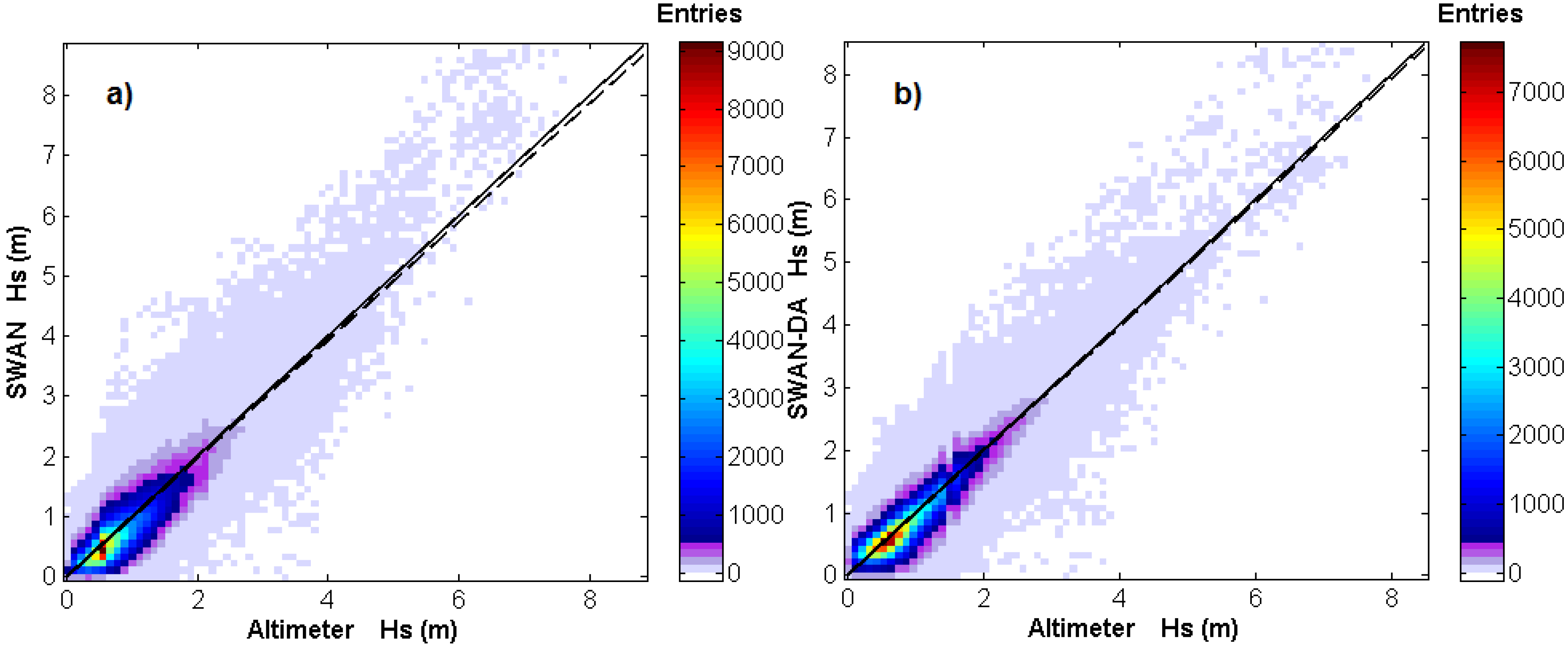
The analysis of the results presented in Table 3 clearly show that by applying the DA scheme all the statistical parameters are improved, while significant improvements in terms of the parameters MAE, RMSE, SI, and R are noticed. Scatter diagrams have been also designed and they are presented in Figure 3.

Table 3. Statistical results obtained for the Hs values simulated with SWAN and the Hs values obtained after the application of the DA method, against altimeter measurements used for validation across the Black Sea, results corresponding to the 15-year time interval (1999–2013).

Parameter	MeanObs (m)	MeanSim (m)	Bias (m)	MAE (m)	RMSE (m)	SI	R	S	N
SWAN Hs (m)	1.04	0.97	−0.07	0.27	0.35	0.35	0.88	0.98	316,920
SWAN-DA Hs (m)		1.01	−0.03	0.21	0.29	0.28	0.91	0.99

Table 3. Statistical results obtained for the Hs values simulated with SWAN and the Hs values obtained after the application of the DA method, against altimeter measurements used for validation across the Black Sea, results corresponding to the 15-year time interval (1999–2013).

Parameter	MeanObs (m)	MeanSim (m)	Bias (m)	MAE (m)	RMSE (m)	SI	R	S	N
SWAN Hs (m)	1.04	0.97	−0.07	0.27	0.35	0.35	0.88	0.98	316,920
SWAN-DA Hs (m)		1.01	−0.03	0.21	0.29	0.28	0.91	0.99

Figure 3. Scatter diagrams presenting the observed Hs (data from ENVISAT, Topex and Cryosat-2 satellites) against the predicted Hs computed using the SWAN model without DA (a) and with DA (b), corresponding to the 15-year period (1999–2013). The different colors indicate different quantities of data in the single pixels. The solid lines denote the perfect fit to the modelled and observed values and the dashed lines represent the best-fit slope.

Figure 3. Scatter diagrams presenting the observed Hs (data from ENVISAT, Topex and Cryosat-2 satellites) against the predicted Hs computed using the SWAN model without DA (a) and with DA (b), corresponding to the 15-year period (1999–2013). The different colors indicate different quantities of data in the single pixels. The solid lines denote the perfect fit to the modelled and observed values and the dashed lines represent the best-fit slope.

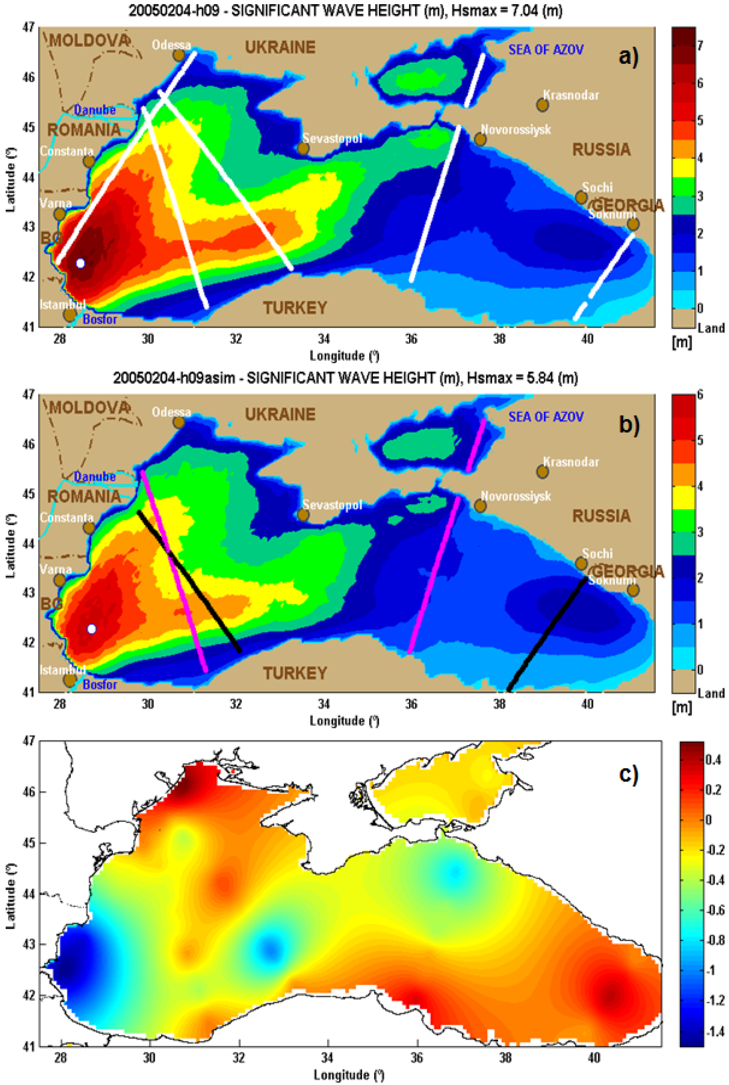
In Figure 4, an example of the results obtained before and after the application of the DA technique is presented. Thus, Figure 4a illustrates the results of the SWAN simulations in the Black Sea in terms of significant wave height scalar fields for the time frame 2005.02.04-h09. In the same Figure 4a, the satellite tracks for the entire day 4 February 2005, corresponding to the data considered for the assimilation process are represented with white color. Figure 4b presents the new significant wave height scalar fields, as obtained after applying the DA technique, and also the satellite tracks considered for validations, which are represented with black and magenta color, respectively. Finally, Figure 4c illustrates the differences in terms of the H_s scalar fields, which means significant wave height with DA minus significant wave height without DA. Comparisons along the satellite tracks, SWAN without DA, SWAN with DA and satellite measurements (ENVISAT and TOPEX) are presented in Figure 5. The graphs clearly show that after assimilation the values of the parameter H_s are significantly closer to the measurements.

Figure 4. Significant wave height (Hs) scalar fields corresponding to the time frame 2005.02.04-h09: (a) SWAN Hs fields (without DA), the satellite tracks considered for the assimilation process (corresponding to the entire day on 4 February 2005) are represented with white color; (b) SWAN Hs fields with DA, the satellite tracks considered for the validation process (ENVISAT—tracks with magenta color, TOPEX—tracks with black color); and (c) Hs scalar fields, differences Hs with DA against Hs without DA.

Figure 4. Significant wave height (Hs) scalar fields corresponding to the time frame 2005.02.04-h09: (a) SWAN Hs fields (without DA), the satellite tracks considered for the assimilation process (corresponding to the entire day on 4 February 2005) are represented with white color; (b) SWAN Hs fields with DA, the satellite tracks considered for the validation process (ENVISAT—tracks with magenta color, TOPEX—tracks with black color); and (c) Hs scalar fields, differences Hs with DA against Hs without DA.

Figure 5. Comparisons between: H_s measured, H_s simulated with SWAN, and H_s obtained after applying DA along the satellite tracks, corresponding to the entire day 4 February 2005. (a) Tracks of ENVISAT; (b) Tracks of TOPEX.

Figure 5. Comparisons between: H_s measured, H_s simulated with SWAN, and H_s obtained after applying DA along the satellite tracks, corresponding to the entire day 4 February 2005. (a) Tracks of ENVISAT; (b) Tracks of TOPEX.

3. Wave Energy Assessments

3.1. Analyses of the Wave Energy Distribution in the Geographical Space of the Black Sea

Considering now the results coming from the SWAN simulations with DA, corresponding to the 15-year period (1999–2013), an analysis concerning the main wave energy patterns in the basin of the Black Sea has been carried out. First, the spatial distribution of the mean wave power for the entire period considered was computed as the average of the 43,832 spatial distribution records that represent the model output for the entire 15-year period with a temporal resolution of 3 h. From this total amount of data, the information that is necessary to compute the average annual and seasonal values has been extracted, as well as the information corresponding to each month of the year. On this basis, comparisons have been also performed against the corresponding data as resulting from the SWAN model simulations without DA, computing in this way the differences in terms of the wave power scalar fields with and without DA. Some of the most relevant results will be presented and discussed next.

Thus, Figure 6a,c present the mean values of the wave power computed for the total time interval and for the winter time, respectively. At this point, it has to be highlighted that in the present work the winter time represents in fact the six-month interval from October to March. Both spatial distributions presented in Figure 6a,c indicate that the western side, and especially the southwestern side of the Black Sea, has a higher wave power in comparison with the eastern side. On the other hand, we can also notice that it can be identified in the northeastern side of the sea a relatively small area where the values of the wave power are comparable with those from the western side. As illustrated by Figure 6, the maximum value of the mean power is 4.5 kW/m for the total period and 7.1 kW/m for the winter season, the position of this maximum being located in both situations in almost the same place in the southwestern side of the sea and these positions are also represented in Figure 6a,c with a small white circle.

Figure 6. Mean wave power fields corresponding to the time period 1999–2013, as resulted from the SWAN simulations with DA: (a) total data, and (c) winter season; Differences, mean wave power fields with DA against mean wave power as resulted from the SWAN simulations without DA: (b) total data, and (d) winter season.

Figure 6. Mean wave power fields corresponding to the time period 1999–2013, as resulted from the SWAN simulations with DA: (a) total data, and (c) winter season; Differences, mean wave power fields with DA against mean wave power as resulted from the SWAN simulations without DA: (b) total data, and (d) winter season.

As reflected by Figure 6b,d, the DA process induces more significant changes in the wave power field, especially in the southwest and in the center of the Black Sea basin. As regards the total time, we can notice that the average values in the case with DA are all over the basin of the Black Sea greater than those without DA. This is because all the differences presented in Figure 6b are positive. The maximum values of these differences are around 0.5 kW/m and they are located in the south, in the southwest and in the center of the sea basin, while the smallest values can be encountered in the Sea of Azov and in the west of the basin. On the other hand, in the wintertime, these differences are both positive and negative. Thus, the highest values, which can reach now 1 kW/m, are still noticed in the southwest and in the center of the sea, in the west these values are around 0.5 kW/m or less, while in the east these differences become negative.

From the comparison of the spatial distributions of the mean wave power, presented in Figure 6a,c, we can notice that the wave power is considerably higher in the winter in relationship with the total time period. On the other hand, from the analysis of the monthly mean wave power fields, computed as average of all the records corresponding to each month of the year from the entire 15-year time interval, there have been identified as having the highest average wave power the months November, December, January, and February. The corresponding results are illustrated in Figure 7. Such average values were computed for all months, but only the results corresponding to these four more energetic months are presented here. As illustrated by Figure 7, February presents the highest value of the mean wave power (9.7 kW/m). A significant difference can be noticed between February and March (not presented) the maximum wave power value that resulted in March being 5.3 kW/m.

Figure 7. Mean wave power fields corresponding to the time period 1999–2013, as resulted from the SWAN simulations with DA for the months: (a) November; (b) December; (c) January; and (d) February.

Figure 7. Mean wave power fields corresponding to the time period 1999–2013, as resulted from the SWAN simulations with DA for the months: (a) November; (b) December; (c) January; and (d) February.

All the monthly distributions presented in Figure 7 follow in general the same pattern for the more energetic areas, characterized by more elevated values in the west and the southwest of the basin and also in the small area identified in the northeast. We can also notice that only in November the maximum is located in this small area.

Another analysis considering the results of 15-year of wave model simulations is related to the percentage, from the total, of the wave power conditions greater than 4 kW/m. The selection of this threshold is based on two reasons. First, it is because for this value of the wave power most of the existing wave energy converters can produce electric power in relatively good conditions, this depending also on the distribution of the wave power along the sea states defined in terms of significant wave height and wave energy period. The second reason is due to the fact that 4 kW/m represents the higher entire value of the wave power corresponding to the results presented in Figure 6a for the total time. Thus, from this perspective, some results are provided in Figure 8 for total time and winter period, respectively. As we can notice from this figure, in the case of the total time the highest percentage (24%) occurs in the southwestern zone, but on the other hand for the winter time the highest percentage (34%) corresponding to the wave power values over 4 kW/m occur in an extended geographical space in the western side of the sea basin and also in the zone from the eastern side previously identified as being more energetic.

Figure 8. Results of the 15-year wave simulations (1998–2013); (a) Geographical distribution in percentage of the wave power greater than 4 kW/m, total period; (b) Geographical distribution in percentage of the wave power greater than 4 kW/m, winter period.

Figure 8. Results of the 15-year wave simulations (1998–2013); (a) Geographical distribution in percentage of the wave power greater than 4 kW/m, total period; (b) Geographical distribution in percentage of the wave power greater than 4 kW/m, winter period.

3.2. Local Analyses of the Wave Energy

Aside from the spatial analysis of the wave energy characteristics, some local analyses have also been performed and they will be next presented. These use the SWAN results in five locations from the Black Sea basin, which can be considered in general as having a relatively high wave power potential. The positions of these reference points are illustrated in Figure 1, while the points coordinates and the corresponding water depths are provided in Table 4. We can notice that some points are located in deep water (P3 and P5) while others in intermediate water depth (P1, P2, and P4).

Table 4. Characteristics of the parameters H_s and P_W in the five reference points considered.

Point	Position	Depth (m)	Hs-mean ± std.dev. (m)	Hs-max (m)	PW-mean (kW/m)	PW-max (kW/m)
P1	29.57° E/44.52° N	47	0.98 ± 0.71	7.80	2.90	246.7
P2	28.84° E/43.90° N	43	0.94 ± 0.70	8.14	2.76	272.4
P3	28.70° E/41.62° N	117	1.02 ± 0.86	10.35	4.23	497.7
P4	35.09° E/42.12° N	61	0.48 ± 0.38	5.84	0.93	187.9
P5	37.98° E/44.51° N	220	0.66 ± 0.76	9.60	2.46	475.6

Table 4. Characteristics of the parameters H_s and P_W in the five reference points considered.

Point	Position	Depth (m)	Hs-mean ± std.dev. (m)	Hs-max (m)	PW-mean (kW/m)	PW-max (kW/m)
P1	29.57° E/44.52° N	47	0.98 ± 0.71	7.80	2.90	246.7
P2	28.84° E/43.90° N	43	0.94 ± 0.70	8.14	2.76	272.4
P3	28.70° E/41.62° N	117	1.02 ± 0.86	10.35	4.23	497.7
P4	35.09° E/42.12° N	61	0.48 ± 0.38	5.84	0.93	187.9
P5	37.98° E/44.51° N	220	0.66 ± 0.76	9.60	2.46	475.6

For this analysis the wave parameters considered are the significant wave height (H_s), the wave energy period (T_e), the peak wave direction, and also the wave power. The T_e values represent the output of the SWAN model, and this wave parameter is defined in terms of the spectral moments as (see also [30,31]):

$$T_e=T_{m-1,0}=\frac{m_{-1}}{m_0},m_q={\displaystyle \underset{0}{\overset{\infty }{\int }}{\displaystyle \underset{0}{\overset{2\mathrm{\pi }}{\int }}{\mathrm{\sigma }}^{q}E\left(\mathrm{\sigma },\mathrm{\theta }\right)}}d\mathrm{\sigma }d\mathrm{\theta }$$

(13)

in which m_q is the q order moment of the spectrum. The wave power has been computed by the SWAN model with the relationships given in Equations (4) and (6).

From the results presented in Table 4, we can notice that in the reference point P3, which is located in the south west of the Black Sea, there are encountered the highest values for H_s and P_W. Although the average H_s value corresponding to this point is close to those from P1 and P2, the average value of the parameter P_W is much higher (with over 1.5 kW/m). We can also notice that the maximum values of these two parameters are considerably higher in P3 in comparison with P1 and P2. On the other hand, the point P4, located in the south of the Black Sea, presents the lowest values for the parameters H_s and P_W.

In the case of the reference point P5, which is located in the northeast of the sea basin, the P_W spatial distribution indicates a high seasonal variability and although the average values are not so high, the maximum values are rather elevated, and the standard deviation of the parameter H_s has a value that exceeds the average value, a fact that indicates a high variability in relationship with the average value.

As regards now the H_s directional distributions (Figure 9), since the points are located relatively close to the coast, the range of the wave direction is rather limited. Thus, in the reference points P1, P2, and P5 the wave directions are distributed in a sector of 180° with some clear defined dominant directions. On the other hand, in P3 and P4, the wave direction is distributed within a sector of 90°.

Figure 9. Directional distribution, classes of H_s in the five reference points considered. Results of the simulations with the SWAN wave model in the period 1999–2013. (a) Point P1; (b) Point P2; (c) Point P3; (d) Point P4; (e) Point P5.

Figure 9. Directional distribution, classes of H_s in the five reference points considered. Results of the simulations with the SWAN wave model in the period 1999–2013. (a) Point P1; (b) Point P2; (c) Point P3; (d) Point P4; (e) Point P5.

Scatter diagrams were also designed, presenting the bivariate distributions of the occurrences corresponding to the sea states defined by H_s and T_e (Figure 10). In Figure 10 the colored rectangles represent the number of occurrences, in percentage from the total, which correspond to each rectangular sector with the lengths of 0.5 s in x-direction and 0.5 m in y-direction. The wave power isolines are also represented and they have been calculated using the deep water energy flux approximation (see [32]):

$$P=\frac{\mathrm{\rho }{g}^2}{64\mathrm{\pi }}{T}_e{H}_s^2$$

(14)

where P is the energy flux in watts per meter of crest length, ρ = 1025 kg/m³ is the density of sea water, and g is the acceleration due to gravity.

Figure 10. Scatter diagrams (Hs against Te) for the five reference points considered, corresponding to the period 1999–2013. (a) Point P1; (b) Point P2; (c) Point P3; (d) Point P4; (e) Point P5.

Figure 10. Scatter diagrams (Hs against Te) for the five reference points considered, corresponding to the period 1999–2013. (a) Point P1; (b) Point P2; (c) Point P3; (d) Point P4; (e) Point P5.

Looking at Figure 10 we can also notice that as regards the reference points P1, P2, and P3, the highest number of occurrences is in the vicinity of the isoline of 5 kW/m, while for the other points the highest number of occurrences is placed bellow this isoline. Such kinds of diagrams can provide a coherent image related to the contribution of each sea state to the wave energy expected to be delivered by a wave energy converter (WEC) operating in the area where the computations have been made. On the other hand, this approach can provide a realistic assessment related to the efficiency of various devices that would operate in a certain coastal area.

4. Conclusions

The present work provides a comprehensive picture of the wave energy patterns in the basin of the Black Sea. This is based on 15-year of wave model simulations with assimilation of satellite data and the analysis is focused on the average wave conditions that might be expected in this sea in the total time and winter seasons, respectively. From the analysis of the results presented, it can be noticed that the western side of the sea (and especially the southwestern part) has higher wave energy potential. If we compare now the wave conditions with other European continental coasts, as reflected for example by the results presented in [33,34], or in semi-enclosed sea as the Mediterranean Sea [35,36], we notice that in the European nearshore of the Atlantic Ocean, the wave energy is considerably higher and these locations can be considered indeed very appropriate for the wave energy extraction, some pilot projects being already operational in these areas. On the other hand, if we compare the wave energy from the western side of the Black Sea with that from the Mediterranean Sea, we can notice that, although the Black Sea has a smaller surface, probably due to its active fetch which is usually larger, the energetic potential of the Black Sea appears to be equal, or even sometimes higher, in comparison with that from the Mediterranean Sea.

From this perspective, although most of the existing wave energy converters were designed particularly for the ocean conditions, where the waves are more powerful and the wave periods are larger, the issue of the wave energy extraction in the Black Sea cannot be completely ignored. Moreover, since the wind energy potential in the coastal environment of the Black Sea appears to be quite relevant [7,8], the wind-wave hybrid solutions might become viable in the future, especially from the perspective of the development of the small amplitude wave energy converters. Finally, another important issue that should be taken into account is that the dynamics of the coastal processes in the western side of the Black Sea is usually very high [37,38] and the marine energy farms can play also an active role in the coastal protection.

References

1. Ovchinnikov, I.; Popov, M.; Yu, I. Evolution of the cold intermediate layer in the Black Sea. Oceanology 1987, 27, 555–560. [Google Scholar]
2. Tolmazin, D. Changing coastal oceanography of the Black Sea in northwestern shelf. Prog. Oceanogr. 1985, 15, 217–276. [Google Scholar] [CrossRef]
3. Enriquez, C.E. Mesoscale Circulation in the Black Sea: A Study Combining Numerical Modelling and Observa-tions. Ph.D. Thesis, The University of Plymouth, Devon, UK, 2005; p. 257. [Google Scholar]
4. Filippov, D.M. The cold intermediate layer in the Black Sea. Oceanology 1965, 5, 47–52. [Google Scholar]
5. Efimov, V.V.; Anisimov, A.E. Climatic parameters of wind_field variability in the Black Sea region: Numerical reanalysis of regional atmospheric circulation. Izv. Atmos. Oceanic Phys. 2011, 47, 350–361. [Google Scholar] [CrossRef]
6. Valchev, N.; Davidan, I.; Belberov, Z.; Palazov, A.; Valcheva, N. Hindcasting and assessment of the western Black Sea wind and wave climate. J. Environ. Prot. Ecol. 2010, 11, 1001–1012. [Google Scholar]
7. Onea, F.; Rusu, E. An evaluation of the wind energy in the north-west of the Black Sea. Int. J. Green Energy 2014, 11, 465–487. [Google Scholar] [CrossRef]
8. Onea, F.; Rusu, E. Wind energy assessments along the Black Sea basin. Meteorol. Appl. 2014, 21, 316–329. [Google Scholar] [CrossRef]
9. Rusu, L.; Butunoiu, D.; Rusu, E. Analysis of the extreme storm events in the Black Sea considering the results of a ten-year wave hindcast. J. Environ. Prot. Ecol. 2014, 15, 445–454. [Google Scholar]
10. European Commission. Energy Roadmap 2050; European Commission: Brussels, Belgium, 2011; p. 885. [Google Scholar]
11. European Commission. Technology Map of the SET-Plan; European Commission: Brussels, Belgium, 2013; pp. 1018–5593. [Google Scholar]
12. Rusu, E. Wave energy assessments in the Black Sea. J. Mar. Sci. Technol. 2009, 14, 359–372. [Google Scholar] [CrossRef]
13. Rusu, E. Evaluation of the wave energy conversion efficiency in various coastal environments. Energies 2014, 7, 4002–4018. [Google Scholar] [CrossRef]
14. Booij, N.; Ris, R.C.; Holthuijsen, L.H. A third generation wave model for coastal regions. Part 1: Model description and validation. J. Geophys. Res. 1999, 104, 7649–7666. [Google Scholar]
15. Janssen, P.A.E.M. Quasi-linear theory of wind-wave generation applied to wave forecasting. J. Phys. Oceanogr. 1991, 21, 1631–1642. [Google Scholar] [CrossRef]
16. Hasselmann, K.; Barnett, T.P.; Bouws, E.; Carlson, H.; Cartwright, D.E.; Enke, K.; Ewing, J.A.; Gienapp, H.; Hasselmann, D.E.; Kruseman, P.; et al. Measurements of wind—Wave growth and swell decay during the Joint North Sea Wave Project (JONSWAP). Dtsch. Hydrogr. Z. Suppl. 1973, 12, A8. [Google Scholar]
17. Stelling, G.S.; Leendertse, J.J. Approximation of convective processes by cyclic AOI methods. In Proceeding of the 2nd International Conference on Estuarine and Coastal Modeling (ASCE), Tampa, FL, USA, 13–15 November 1992; pp. 771–782.
18. Rusu, L.; Bernardino, M.; Guedes Soares, C. Wind and wave modelling in the Black Sea. J. Oper. Oceanogr. 2014, 7, 5–20. [Google Scholar]
19. Cherneva, Z.; Andreeva, N.; Pilar, P.; Valchev, N.; Petrova, P.; Guedes Soares, C. Validation of the WAMC4 wave model for the Black Sea. Coastal Eng. 2008, 55, 881–893. [Google Scholar] [CrossRef]
20. Ardhuin, F.; Bertotti, L.; Bidlot, J.-R.; Cavaleri, L.; Filipetto, V.; Lefevre, J.M.; Wittmann, P. Comparison of wind and wave measurements and models in the Western Mediterranean Sea. Coastal Eng. 2007, 34, 526–541. [Google Scholar] [CrossRef]
21. Dykes, J.D.; Wang, D.W.; Book, J.W. An evaluation of a high-resolution operational wave forecasting system in the Adriatic Sea. J. Mar. Syst. 2009, 78, 255–271. [Google Scholar] [CrossRef]
22. Rusu, E.; Onea, F. Evaluation of the wind and wave energy along the Caspian Sea. Energy 2013, 50, 1–14. [Google Scholar] [CrossRef]
23. Kalnay, E. Atmospheric Modeling, Data Assimilation and Predictability; Cambridge University Press: Cambridge, UK, 2003; p. 341. [Google Scholar]
24. Reichle, R.H. Data assimilation methods in the Earth sciences. Adv. Water Resour. 2008, 31, 1411–1418. [Google Scholar] [CrossRef]
25. Daley, R. Atmospheric Data Analysis; Cambridge University Press: New York, NY, USA, 1991; p. 457. [Google Scholar]
26. Lionello, P.; Günther, H.; Janssen, P.A.E.M. Assimilation of altimeter data in a global third-generation wave model. J. Geophys. Res. 1992, 97, 14453–14474. [Google Scholar] [CrossRef]
27. Thomas, J.P. Retrieval of energy spectra from measured data for assimilation into a wave model. Q. J. R. Meteorol. Soc. 1988, 114, 781–800. [Google Scholar] [CrossRef]
28. Greenslade, D.J.M.; Young, I.R. The impact of inhomogenous background errors on a global wave data assimilation system. J. Atmos. Ocean Sci. 2005, 10, 61–93. [Google Scholar] [CrossRef]
29. Rusu, L. Wave modelling with data assimilation to evaluate the wave energy paterns in the Black Sea. In Proceedings of the 15th International Multidisciplinary Scientific Geo Conference (SGEM2015)—Renewable Energy Sources and Clean Technologies, Albena, Bulgaria, 17–26 June 2015.
30. Cornett, A.M. A global wave energy resource assessment. In Proceedings of the 18th International Offshore and Polar Engineering Conference (ISOPE), Vancouver, BC, Canada, 6–11 July 2008; pp. 318–323.
31. ABP Marine Environmental Research Ltd. Atlas of UK Marine Renewable Energy Resources; Technical Report, Report No. R.1106 Prepared for the UK Department of Trade and Industry; ABP Marine Environmental Research Ltd.: Southampton, UK, 2004. [Google Scholar]
32. Vicinanza, D.; Contestabile, P.; Ferrante, V. Wave energy potential in the north-west of Sardinia (Italy). Renew. Energy 2013, 50, 506–521. [Google Scholar] [CrossRef]
33. Rusu, L.; Onea, F. Assessment of the performances of various wave energy converters along the European continental coasts. Energy 2015, 82, 889–904. [Google Scholar] [CrossRef]
34. Silva, D.; Rusu, E.; Guedes Soares, C. Evaluation of various technologies for wave energy conversion in the Portuguese nearshore. Energies 2013, 6, 1344–1364. [Google Scholar] [CrossRef]
35. Vicinanza, D.; Cappietti, L.; Ferrante, V.; Contestabile, P. Estimation of the wave energy in the Italian offshore. J. Coastal Res. 2011, SI 64, 613–617. [Google Scholar]
36. Iuppa, C.; Cavallaro, L.; Vicinanza, D.; Foti, E. Investigation of suitable sites for wave energy converters around Sicily (Italy). Ocean Sci. Discuss. 2015, 12, 315–354. [Google Scholar] [CrossRef]
37. Zanopol, A.; Onea, F.; Rusu, E. Evaluation of the coastal influence of a generic wave farm operating in the Romanian nearshore. J. Environ. Prot. Ecol. 2014, 15, 597–605. [Google Scholar]
38. Zanopol, A.; Onea, F.; Rusu, E. Coastal impact assessment of a generic wave farm operating in the Romanian nearshore. Energy 2014, 72, 652–670. [Google Scholar] [CrossRef]