Optimal Real-Time Scheduling for Hybrid Energy Storage Systems and Wind Farms Based on Model Predictive Control

Abstract

Energy storage devices are expected to be more frequently implemented in wind farms in near future. In this paper, both pumped hydro and fly wheel storage systems are used to assist a wind farm to smooth the power fluctuations. Due to the significant difference in the response speeds of the two storages types, the wind farm coordination with two types of energy storage is a problem. This paper presents two methods for the coordination problem: a two-level hierarchical model predictive control (MPC) method and a single-level MPC method. In the single-level MPC method, only one MPC controller coordinates the wind farm and the two storage systems to follow the grid scheduling. Alternatively, in the two-level MPC method, two MPC controllers are used to coordinate the wind farm and the two storage systems. The structure of two level MPC consists of outer level and inner level MPC. They run alternatively to perform real-time scheduling and then stop, thus obtaining long-term scheduling results and sending some results to the inner level as input. The single-level MPC method performs both long- and short-term scheduling tasks in each interval. The simulation results show that the methods proposed can improve the utilization of wind power and reduce wind power spillage. In addition, the single-level MPC and the two-level MPC are not interchangeable. The single-level MPC has the advantage of following the grid schedule while the two-level MPC can reduce the optimization time by 60%.

1. Introduction

With the increasing penetration of wind energy into power grids, the negative influences of wind farms are non-negligible [1,2]. The variability and intermittence of wind power cause fluctuation of the voltage and frequency of the grid, affecting the safety of the power grid [3,4]. Energy storage systems have been verified to be an effective method for overcoming these deficiencies [5,6,7]. The system that coordinates a wind farm with energy storage systems can be dispatched into power grids, which is similar to that of a conventional energy plant [8]. Energy storage systems can be classified into two general categories: high power density and high energy density types [9,10,11]. Moreover, energy storage systems can be classified as fast response or slow response depending on the response time [12]. Because smoothing the complex fluctuation of wind power using a single type of energy storage is difficult, hybrid energy storage systems may be a better choice for wind farms for both technical and economic reasons [13,14].

Wind farm scheduling can be classified into the day-ahead scheduling and the real-time scheduling according to the influence of wind power on the grid [15]. The day-ahead scheduling is employed to address the long-term influence, and the real-time scheduling is applied to address the short-term influence. Both the day-ahead and the real-time scheduling have drawn much attention in recent years [16,17]. The approaches of model predictive control (MPC), fuzzy logic control (FLC) [18], dynamic programming [19] and mixed-integer nonlinear programming (MINLP) [20] have been used to perform real-time scheduling. The MPC algorithm has been widely used in industry cases since its first application in chemical process industry in 1990. Recently, MPC has been adopted in power and renewable energy systems as well [21,22,23,24,25,26,27,28]. MPC has two main advantages: the simplicity of handling complex constraints and real-time control based on rolling horizon optimization. Indeed, MPC transforms a control problem into an optimization problem [29]. First, MPC solves a finite horizon optimization problem with some future information at the sampling time, and only the results for the current time are used. The overall procedure is then repeated at the next sampling time [18]. The optimal results closely describe the actual situation because of the look-ahead characteristic of MPC. On the other hand, other conventional control approaches such as the proportional integral derivative (PID) method and fuzzy control methods can also be implemented in real time scheduling. However, the PID and fuzzy control do not belong to optimal algorithm, and their scheduling results are less than the results of MPC. Meanwhile, in this paper the Equations (15) and (16) are logic constrains, these logic constraints can be easily fulfilled using a CPLEX optimal tool, which is a common tool used in building MPC model. In contrast, they are hard to perform with the PID and fuzzy controller methods. Moreover, the MPC method can easily handle complex constraints, while the PID and fuzzy control have difficulty in handling them.

The application of the MPC method to control energy storage systems and wind farms has been studied by many investigators. In the research, they employed the multi-level hierarchical MPC [24,30,31,32] or one-level MPC [25,26,27] according to the difference in control architectures. Wei et al. proposed a two-level hierarchical MPC to reduce the MPC optimization time [24]. In this application, energy storage is used to coordinate wind-solar subsystems to optimize the production of desalinated water and the water and storage requirement is met. The upper level is modeled as a long-timescale problem, while the lower level is a short-timescale problem. The optimized upper level results are used as the input of the lower level. In [25], the architecture of the MPC is single-level. A wind-battery optimization model is established for a storage system and wind farm to conduct scheduling in the same manner as a traditional plant does. Other literature is available on real-time scheduling involving fuzzy logic control and dynamic programming. Lei et al. presented a two-level dynamic programming to manage a wind farm and a storage system [33], in which the upper level is implemented over the whole period to obtain the reference trajectory and the lower level is implemented for real-time operation. In [28], a combination of the MPC method with fuzzy logic control was proposed, in which MPC is used for real-time control to achieve the optimization objective, and a fuzzy logic controller adjusts the power reference to increase the lifetime of the storage system.

In [24], the author took advantage of two-time-scale property of the dynamics of the integrated system to improve the computational efficiency of the control problem formulation. This merit has reduced the computation burden of the method, and now it can be implemented in real time system. However, we think this method could exist a demerit in running stability. In extreme condition, the prediction error could lead to the optimal mode failure in finding feasible solution. In [25], the merit of the paper is presented with a third-order battery model and a state space is used to describe the battery model. Additionally, author has also found that the prediction horizon of MPC is an important parameter that contributes to the scheduling performance. The demerit of this paper could be that the battery energy storage system (BESS) charge/discharge frequency is relatively high. Thus, the limit constrain of charge/discharge frequency should be added in this model. In [28], the merit of the method is that MPC method is combined with fuzzy logic control (FLC) method to control the wind farm and energy storage. The combination of the two methods is a novel way, and the results have demonstrated that the wind farm revenue has been improved by 3%. The demerit of this paper is that authors adopt single storage rather than two types of storage. The hybrid storage has more advantages than single type energy storage, and these advantages can assist the wind farm in following scheduling. In [33], the author has succeeded in overcoming the dilemma of the conflict between long horizon and prediction accuracy. The method is very useful in controlling sophisticated system consisted by wind farm and energy storage. However, we think there was a minor unreasonable description in the battery model. We believe that the battery ought is to occupy only one of the three states at any given time: charge, discharge, or shut-down, while according to the battery mode (Equation (5)) a battery can be in charge and discharge state simultaneously, therefore we think the author may have neglected this minor point in his model.

Although many researchers have investigated the management of a wind farm with a single type of storage based on MPC, few researchers have studied a wind farm with a hybrid storage system based on MPC, especially when the hybrid storage system includes pumped hydro storage. A battery storage system may be more practical than a pumped hydro storage system; however, there are some special cases in which a battery storage system cannot replace a pumped hydro storage system. For example, on an isolated island, pumped hydro storage serves as not only energy storage but also a reservoir for local citizens. Moreover, the pumped hydro storage system has some advantages such as large storage capacity, high efficiency, mature construction technology, relatively low capital cost per unit of energy and time-shifting between wind generation and demand profiles. The purpose of this paper is to present two MPC models to be implemented in wind farms with hybrid storage systems including a pumped hydro storage system and a fly wheel system. The MPC models presented consider the power characteristics of wind farms and hybrid storage systems, and the results confirm the efficiency of the MPC model. The merit of propose method is as follows: First, two types of energy are adopted. Second, the MPC method is used to smooth wind power fluctuation. Finally, two type of MPC methods are discussed and compared.

The contributions are listed as follows:

(1)

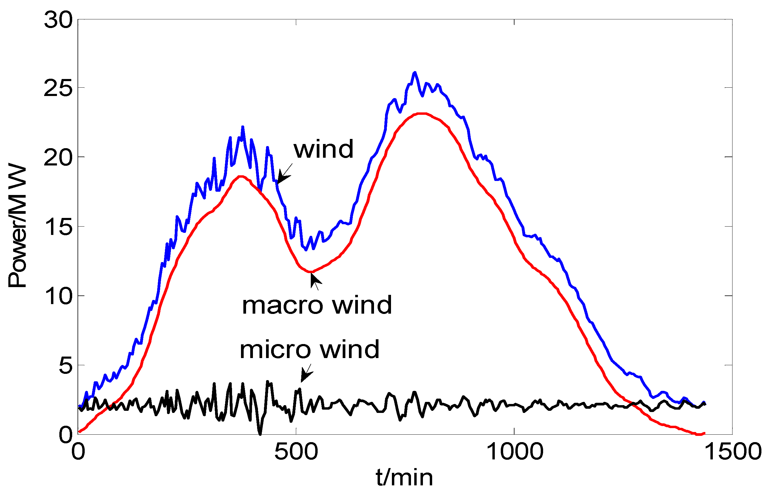
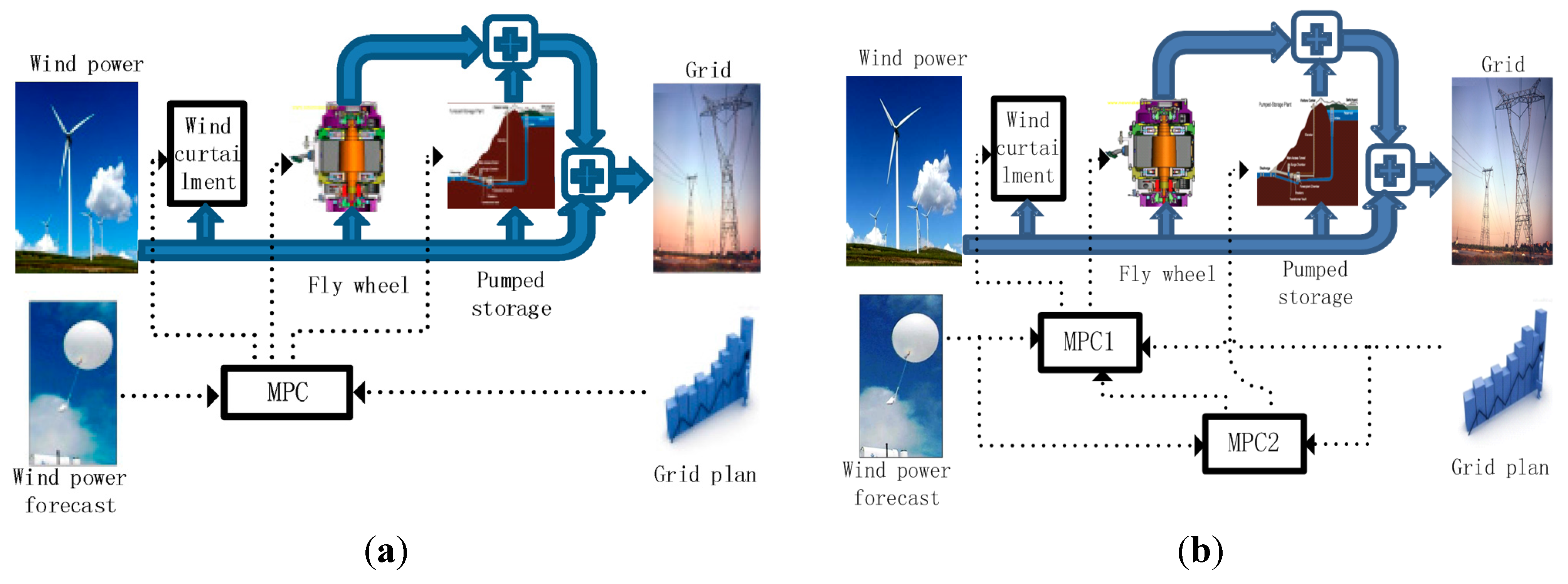
We have adopted a fast response speed energy storage and a slow response speed energy storage to smooth the short term and the long term wind power fluctuations, respectively. Due to the two different response speeds, how to get the two energy storages to cooperate is a problem for real time scheduling. We have exploited the modularity of wind farms based on the MPC method with two types of storage to solve the problem.

(2)

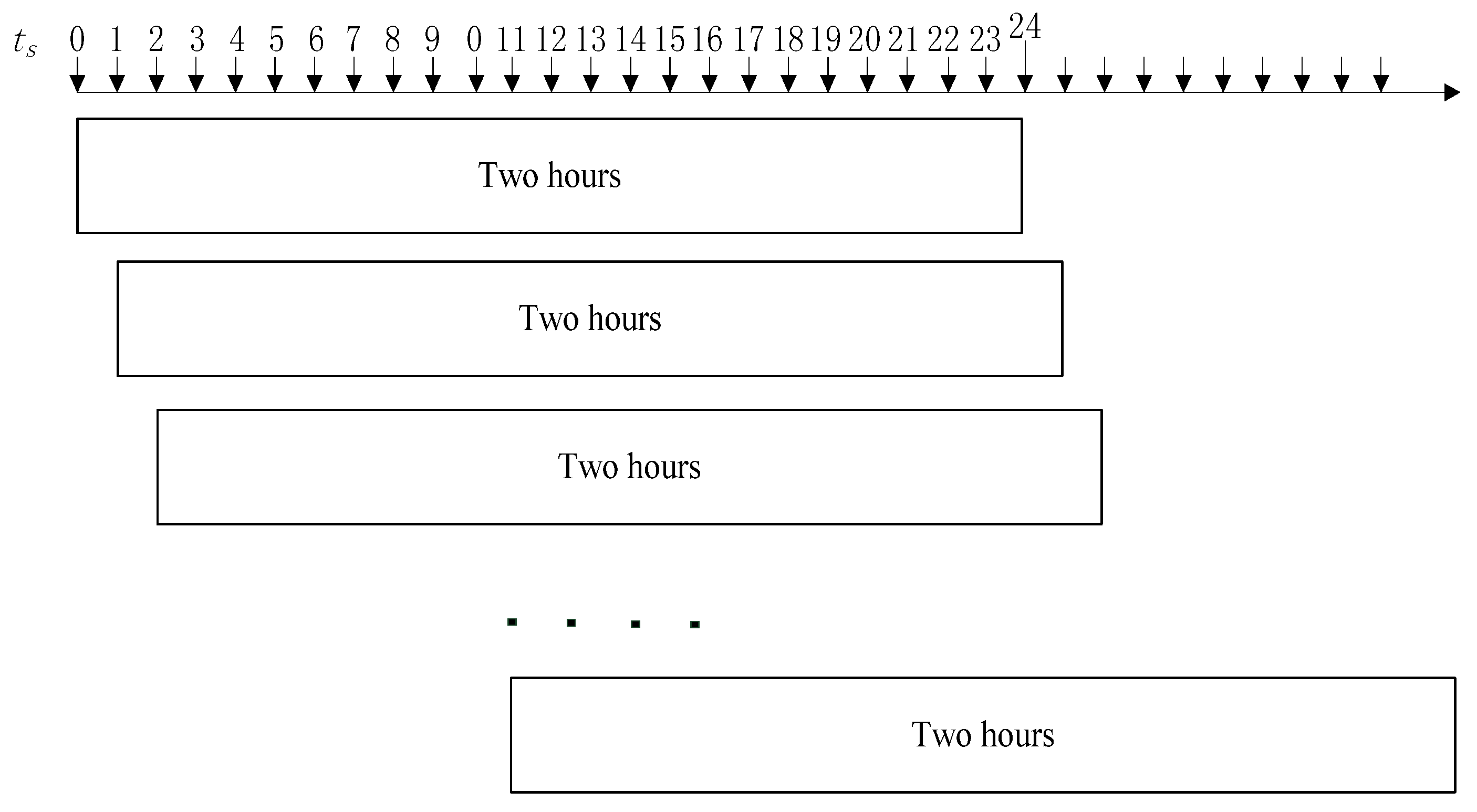
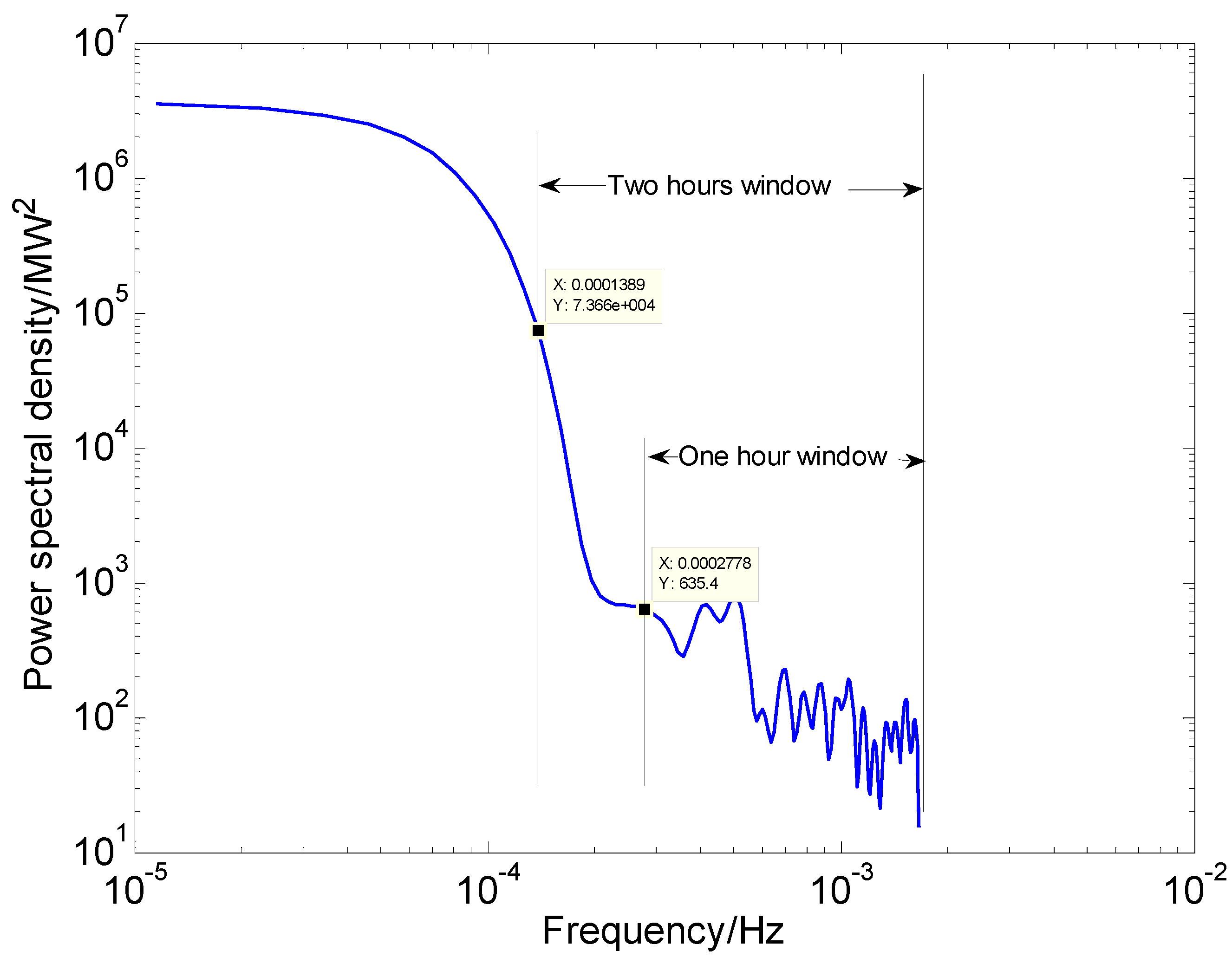
We present that the MPC prediction horizon should be two hours according to the wind farm power spectrum density and prediction error.

(3)

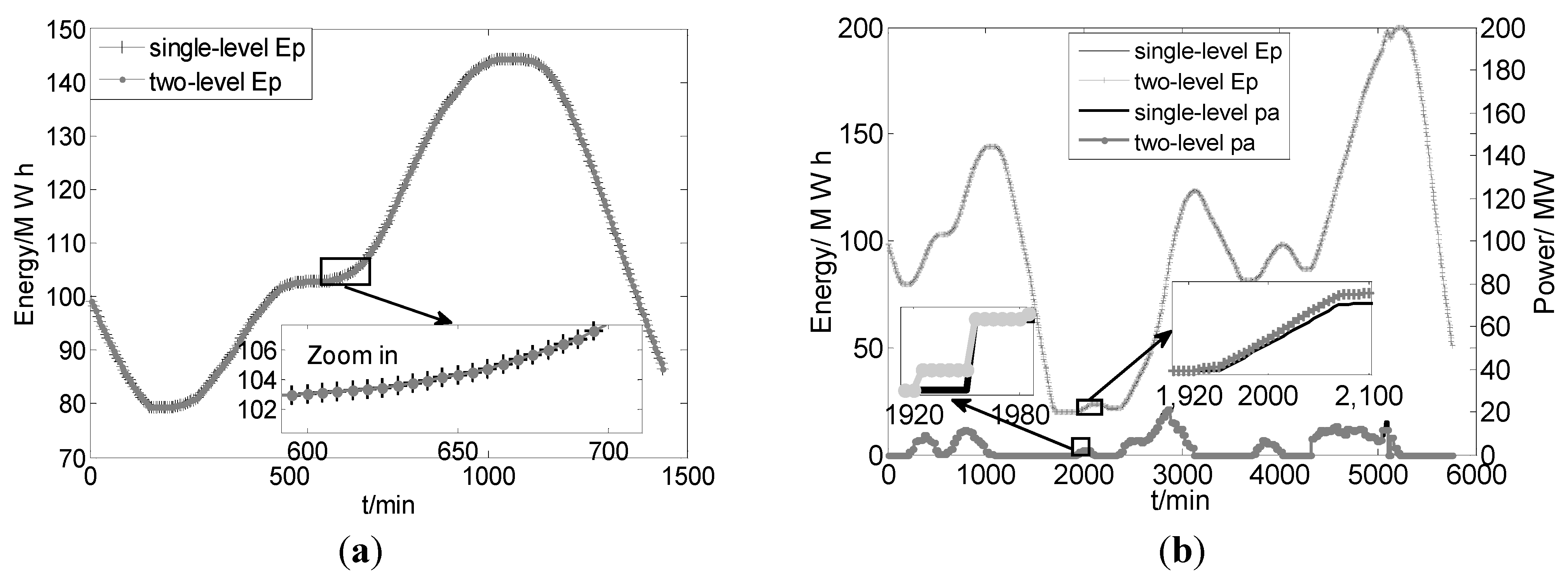
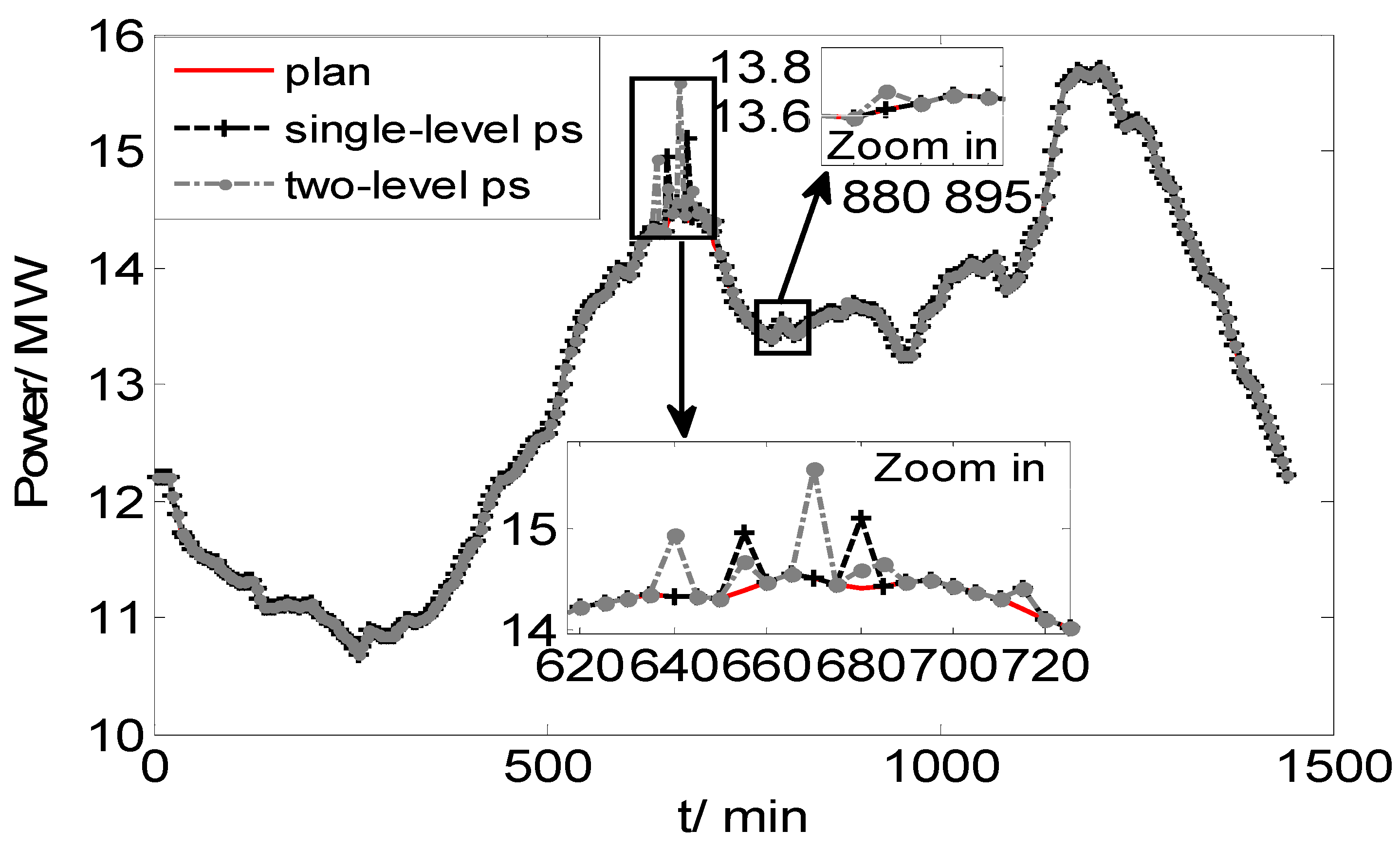
Additionally, we have implemented a two-level MPC to reduce the optimal computation time. The experimental results are close to that of a single-level MPC. The single-level MPC has its own advantages in following the grid plan. The two-level MPC cannot be substituted for single-level MPC, and vice versa.

(4)

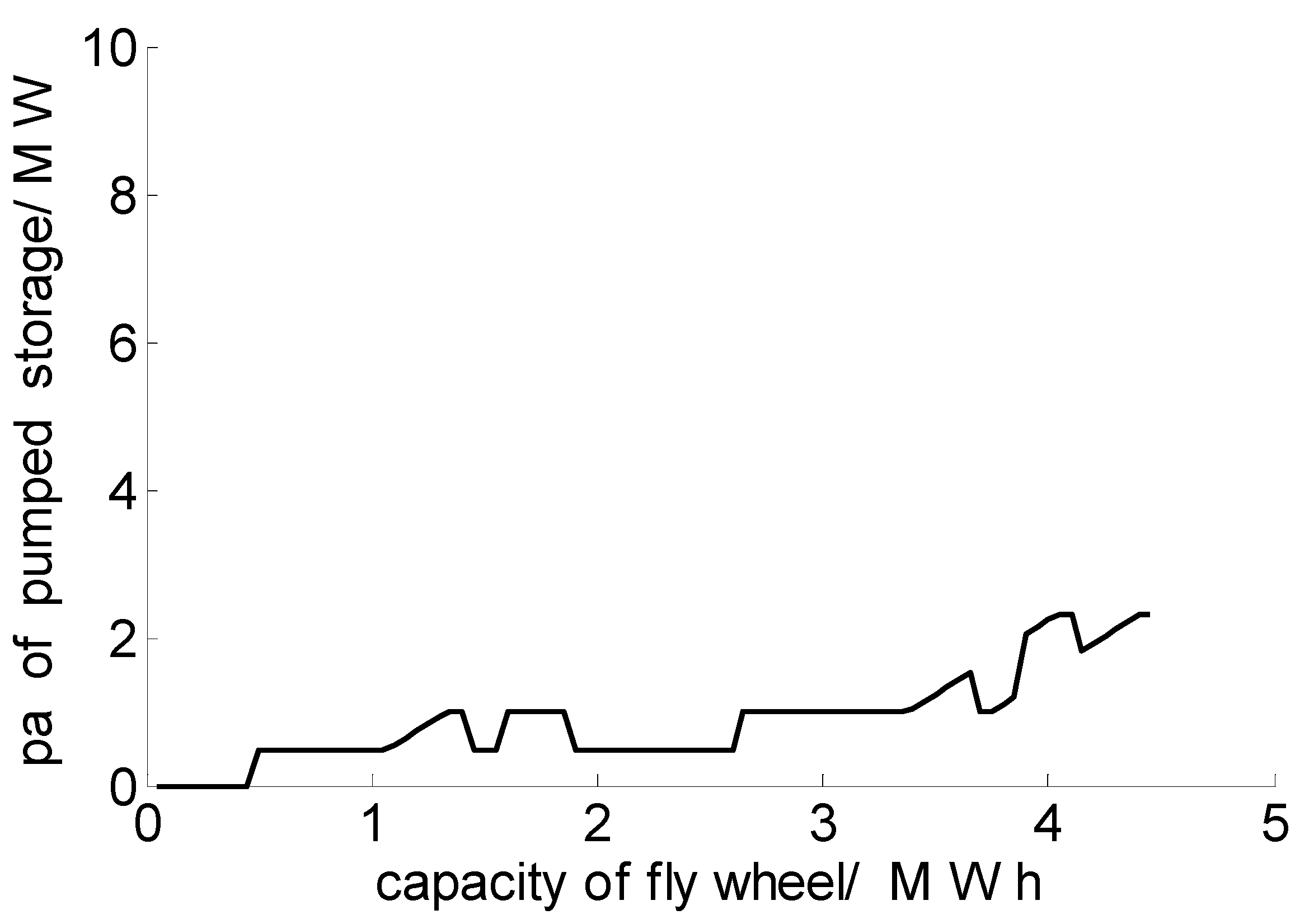
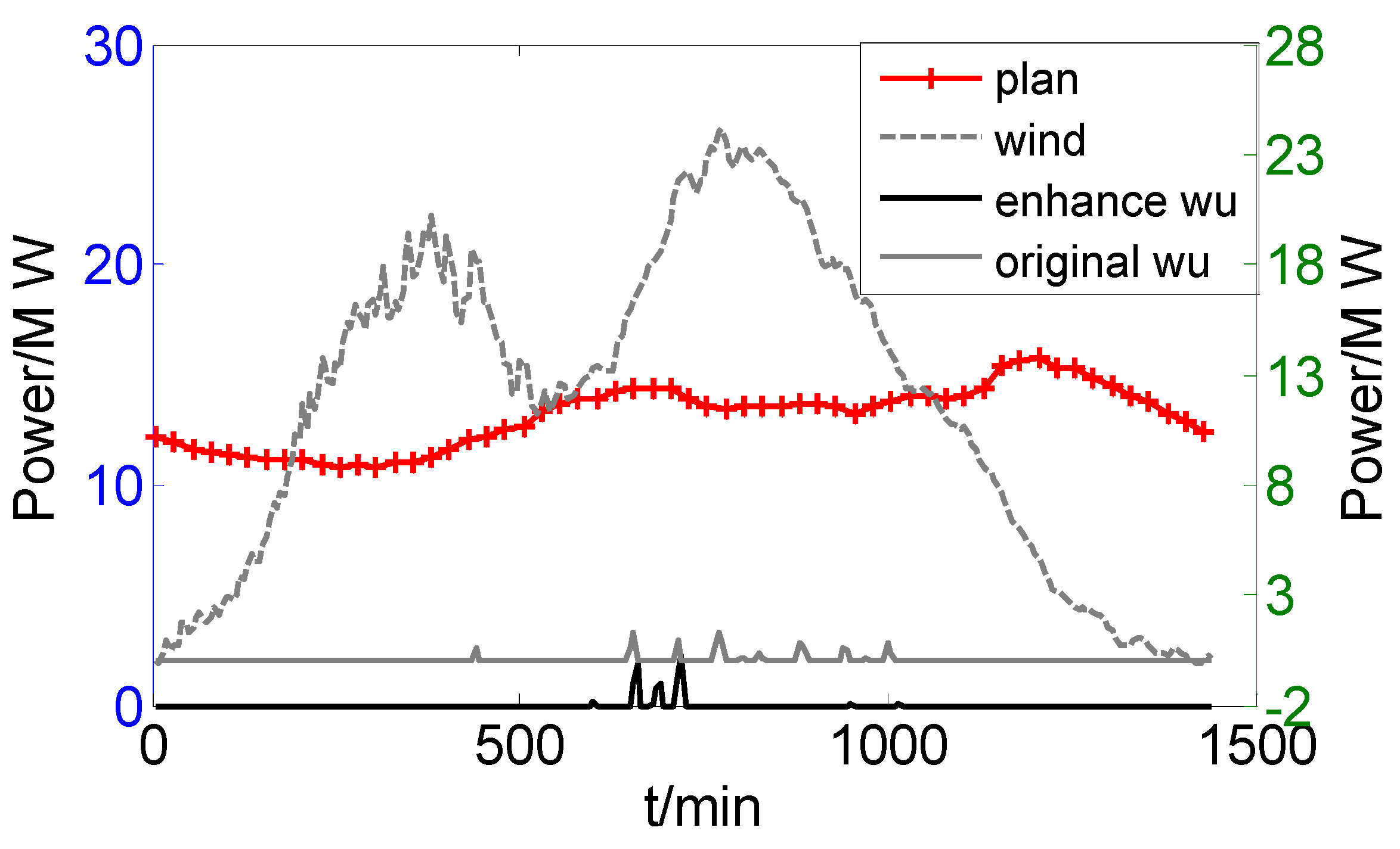
Two sound conclusions are drawn through theory analyses and simulations: One is that the decision values of the pumped storage are not sensitive to the flywheel capacity. The other is that in some situations, wind power generation being sent to the grid is sacrificed to reduce the wind curtailment.

The rest of this paper is organized as follows. In Section 2, the problem to be addressed is described. In Section 3, the system configuration and operating process are given. In Section 4, the proposed system model is described. In Section 5, the numerical results are presented. Finally, the conclusions are presented in Section 6.

2. Problem Description

In this paper, two types of energy storage systems were used to assist a wind farm in smoothing the power fluctuations. One of the key issues is how the two energy storage systems cooperate with each other to perform such power smoothing. In the case of hybrid storage systems, it is important to determine whether common or special decision-making processes exist when a pumped hydro storage system is replaced by another high-energy density storage system. In the following paragraphs, we state the characteristics of wind power and energy storage systems first and then determine the relationships between them. Finally, some useful results and suggestions were obtained.

2.1. Characteristics of Wind Power

Wind power fluctuations consist of two overlapping parts: macro-meteorological fluctuations and micro-meteorological fluctuations [34]. Figure 1 shows the wind fluctuations decomposed into macro-meteorological fluctuations and micro-meteorological fluctuations. From Figure 1, it can be seen that the macro-meteorological fluctuations are relatively slow and smooth and display the trend of wind power generation. In addition, the macro-meteorological fluctuations vary over a large band from 0 to 22 MW, while the micro-meteorological fluctuations are relatively fast and sharp and vary over a relatively narrow band of around 2.5 MW. These observations indicate that two types of storage systems can be used to smooth these two fluctuations. One type of storage is applied to address macro-meteorological fluctuations; in this case, the storage should be a high energy density type with a large power and capacity, but its response speed may be slow. The other type of storage is used to address the micro-meteorological fluctuations; in this case, the storage system requires the capability of rapidly changing power, but a large capacity is not needed.

Figure 1. Decomposition of wind power fluctuations.

Figure 1. Decomposition of wind power fluctuations.

2.2. Characteristics of Typical Energy Storage Systems

Table 1 shows some characteristics of typical energy storage systems. Pumped hydro storage has large power and capacity. However, its response time is long due to the high inertia of water turbines and some security considerations. Additionally, pumped hydro storage may be forbidden from switching from pumped mode to generation mode (and vice versa) within a short time frame [35]. As a result, in this paper, we adopt the reasonable assumption that the pumped hydro storage only has permission to change its operating state once each half hour and that the changing time occurs at the beginning of the half hour (Assumption 1). This assumption can enable pumped hydro storage easy to control and operate safely. Note that for the pumped hydro storage, the term “change state” means that the pumped hydro storage changes the generation mode into pumped mode, and vice versa. Moreover, the term also means that the pumped hydro storage changes the power value of generation or pumping. For fly wheel, the meaning of the term is similar to that for pumped hydro storage.

The fly wheel has low capacity and fast response speed, as indicated in Table 1. The response time of a fly wheel is 0.05 s. For conventional scheduling processes, the fly wheel is regarded as a fast storage device, and it can change its operating state at any scheduling time (Assumption 2).

In this paper, we assume that the scheduling interval is five minutes and the scheduling horizon is one day or 24 h (Assumption 3).

Table 1. Characteristics of typical energy storage types.

Type	Power (MW)	Energy (MWh)	Energy Density (Wh/kg)	Power Density (W/kg)	Efficiency (%)	Respond time (s)	Life (year or cycle)
Pumped hydro	0–1800	>200	0.5–1.5	-	75	10–600	50 y
Compressed air	0–300	0–105	30–60	10–100	64	1–600	30 y
SMES	0–10	0–1	30–100	104–105	95	0.005	30 y
Fly wheel	0–5	0–10	5–10	102–103	93	0.05	20 y
Super cap	0–0.3	0–10	<50	0–4000	98	0.05	105 c
Battery	0–50	0–100	30–200	0–500	70	0.02	3000 c

Table 1. Characteristics of typical energy storage types.

Type	Power (MW)	Energy (MWh)	Energy Density (Wh/kg)	Power Density (W/kg)	Efficiency (%)	Respond time (s)	Life (year or cycle)
Pumped hydro	0–1800	>200	0.5–1.5	-	75	10–600	50 y
Compressed air	0–300	0–105	30–60	10–100	64	1–600	30 y
SMES	0–10	0–1	30–100	104–105	95	0.005	30 y
Fly wheel	0–5	0–10	5–10	102–103	93	0.05	20 y
Super cap	0–0.3	0–10	<50	0–4000	98	0.05	105 c
Battery	0–50	0–100	30–200	0–500	70	0.02	3000 c

2.3. Relationship between Wind Power Fluctuation and Storage Systems

As mentioned above, a pumped hydro storage is used to address the macro-meteorological fluctuations. According to Assumption 1, pumped hydro storage changes its work state once each half hour to handle hour-level fluctuations. In addition, it has high power and high capacity characteristics, which assist pumped storage in a smooth wide band of wave. A fly wheel is suitable for dealing with turbulence due to its fast response and low power characteristics.

Substituting compressed air storage for pumped hydro storage appears to be feasible because they have similar parameters. If we substitute a battery for pumped storage, we must consider whether the battery can have both high power and high capacity. Even if a battery system has sufficient power and capacity, the control of the battery will be challenging.

2.4. The Principle of Choosing Prediction Horizon

In this paper, the length of the prediction horizon is depended on the wind power spectrum density and the type of energy storage. We explain the reason as following:

First, for fly wheel storage, it mainly deals with the turbulence due to its fast response speed and low power characteristics. Pumped storage handles macro meteorological fluctuation due to its slow response speed and high power characteristics. Turbulence belongs to minute-level fluctuation, and macro meteorological fluctuation is hour-level or day-level fluctuation. Therefore, the length of the prediction horizon should be hour-level, if the MPC controller is controlling the pumped storage.

Second, the wind farm power spectrum density curve was shown in Figure 2. The macro meteorological fluctuation is relatively low frequency and huge energy, therefore, it should belong to the left part of the curve. The turbulence is relatively high frequency and low energy, so it should belong to the right part of the curve. In Figure 2, “One hour window” means that the length of the MPC prediction horizon is one hour, and “Two hour window” means that the length of MPC prediction horizon is two hours. “One hour window” contains much turbulence and little macro meteorological fluctuation; on the contrary, the “Two hour window” includes much turbulence and some macro meteorological fluctuation. According to these observations, we decided to choose two hours as the MPC prediction horizon.

Finally, we undeniably agree that the three hour solution is also feasible, perhaps it is better than the two hours solution because it contains more macro meteorological fluctuations. However, the prediction accrual of three hours is worse than two hours, which is not beneficial for the real time scheduling. Thus, to balance the prediction accrual and macro meteorological fluctuations, we choose the two hour solution.

Figure 2. Wind power spectrum density curve.

Figure 2. Wind power spectrum density curve.

3. The System Configuration and Operating Process

In this section, two types of system configurations are presented because MPC methods include a conventional MPC (single-level MPC) and a hierarchical MPC (multi-level MPC). The single-level MPC system configuration is shown in Figure 3a, and the two-level MPC system configuration is shown in Figure 3b.

3.1. Single-Level System Configuration and Operating Process

Figure 3a shows that the single-level system consists of a wind farm, a hybrid storage system, a grid, and an MPC controller. The single-level MPC operating process is presented as follows:

First, the MPC obtains the available information, such as the current wind power, forecasted wind power, energy levels in the two energy storage systems, grid plan and working states of the two energy storages (pumped mode or generation mode, charging mode or discharging mode).

Second, the MPC makes optimal decisions based on this information and then implements the actions based on these decisions. Note that only the current time optimal decisions can be made.

The two above-mentioned steps are repeated when the next scheduling time arrives.

Figure 3. System configuration. (a) Single-level system configuration; (b) Two-level system configuration.

Figure 3. System configuration. (a) Single-level system configuration; (b) Two-level system configuration.

3.2. Two-Level System Configuration and Its Operating Process

In hierarchical systems, a number of regulators perform their control actions at different timescales. This approach can be useful when the overall process under control is characterized by slow and fast dynamic behavior [29]. In this paper, pumped hydro storage is a slow form of storage, and the fly wheel is a fast form of storage according to the response time. Therefore, hierarchical MPC is adopted to present the system. This two-level system is composed of a wind farm, a hybrid storage system, a grid, an MPC1 controller, and an MPC2 controller, as shown in Figure 3b.

To understand the cooperation between the MPC1 controller and MPC2 controller, the above-mentioned Assumptions 1, 2 and 3 must be explained in detail. Assumption 3 is that the scheduling interval is 5 min; Assumption 2 is that a fly wheel can change its operating state at any scheduling time interval. Assumption 1 which is crucial, is that the pumped storage cannot change its operating state within a 30 min period until the next 30 min period starts. In other words, pumped hydro storage can change its operating state only at the beginning of the 30 min period and must then maintain its operating state until the 30 min period ends. Note that 30 min corresponds to six scheduling intervals.

The level of MPC 1 is regarded as the inner level or short-term level, and the level of MPC 2 is viewed as the outer level or long-term level. Similar to the conventional hierarchical MPC, in this paper, the long-term MPC operates by first making decisions and then transmitting some decisions to the short-level MPC; that is, information is output from the long-term MPC and then input to the short-term MPC [29].

The two-level MPC operating process is presented as follows:

First, the long-term MPC (MPC 2) runs and makes decisions. Some decisions are then transmitted to the short-term MPC (MPC 1), and further decisions are made.

Second, when the next scheduling interval arrives, the long-term MPC (MPC 2) stops working, and then the short-term MPC (MPC 1) starts working. MPC 1 makes decisions and then performs them.

If a new 30 min period arrives, the first step is repeated, or else the second step is repeated.

There are three ways to communicate between the two controllers. The three ways are Ethernet communications, global system for mobile communications (GSM) and satellite communication technology, respectively. Ethernet communication solution is the cheapest solution among the three ways, and the satellite communication solution is the most expensive solution. We consider the three following implement cases:

If internet is available in the pumped storage station and the fly wheel station then Ethernet communication is recommended.

If the mobile signals exists in the pumped storage station and the fly wheel station, then GSM communication is adopted.

Otherwise, the satellite communication has to be chosen.

In this paper, the two controllers communicate once every five minutes, the speed of above three technologies is fast enough to ensure synchronization of their communication. Meanwhile, it also possible to adopt some protocols in the software to ensure synchronization—for example, the shake hand protocol is a common way to synchronize communication.

4. System Model

In Section 2 (Problem description), the cooperation between the pumped hydro storage and the fly wheel storage was noted. However, the process and details of the cooperation based on rolling optimization have not yet been addressed. The rolling optimization plays a significant role in MPC. When applying MPC method to wind farm and hybrid energy storage, which consist of a fast response speed storage and a slow response speed storage, two types of MPC methods can be implemented. One type is single-level MPC method, and the other is two-level MPC method. For single-level MPC method, a two time scales problem will be met due to two kinds of respond speeds of energy storage. To overcome this problem, single-level MPC method must divide the problem into several situations, and for every situation, a model is used to describe it. The models are carried out in turn according to the situations. In contrast, two-level MPC method is suitable for the hybrid storages. Outer level and inner level MPC run alternatively to perform real-time scheduling. Therefore, in this section, we first analyze the process and details of the cooperation based on two types of MPC method and then attempt to use the optimization model and the state-space method to represent the process in detail. The single-level MPC method is addressed and then two-level MPC method is discussed below.

4.1. Single-Level MPC Method

Before the rolling optimization process is analyzed, some basic information must be given. We assume that the prediction horizon is equal to the control horizon and each of them are two hours. The sample time is 5 min. Let t_s = 0 when MPC controller begins to work, where t_s represents the serial number of the scheduling interval. Two hours are equal to twenty-four scheduling intervals.

The principle of rolling optimization is as follows:

First, at the current time, the MPC controller samples the current interval information, and predicts the information for the next two hours.

Second, MPC performs on-line optimization.

Finally, MPC makes the current time decisions. The above process is repeated on the arrival of the next scheduling interval.

Although the principle is easy and clear, it will become relatively complex, once it is implemented to hybrid energy storage, which has significantly different response speeds. For understanding the principle, we will first analyze a simple example, and then we will explain the complex process. The simple example is that the pumped hydro storage is replaced by a battery. From Table 1, the response speed of the fly wheel is almost equal to that of the battery; therefore, at any scheduling interval, the battery and fly wheel are ready to change their work states according to the optimal results. In contrast, according to assumption 1, the pumped storage is not ready to change its work state at any scheduling interval. In other words, at any scheduling interval, we have the control right to change the fly wheel and battery, but we have almost lost the control right for pumped storage. Therefore, when the principle is applied to the battery and the fly wheel, it is a simple example, and the analysis process is as follows:

MPC controller samples, forecasts, execute on line optimization and produces the results. The MPC controller repeats the above process on the next scheduling interval. Therefore, the MPC controller always performs the same set of actions at any scheduling interval. The process is shown in Figure 4.

Figure 4. Single-level MPC performing rolling optimization (based on battery and fly wheel).

Figure 4. Single-level MPC performing rolling optimization (based on battery and fly wheel).

In Figure 4, at any scheduling interval, the context of MPC controller performing is similar.

When the principle is applied to pumped storage and fly wheel, the process will become relatively complex, due to the control right of the pumped storage. According to Assumption 1, the pumped storage is under control at every starting half an hour, consequently, when t_s is 0, 6, 12, 18, 24…, both the pumped storage and the fly wheel are under control. The control right situation is similar to that of battery and fly wheel. Any other time, the two situations are different. The details are shown in Figure 5.

Figure 5 schematically shows the process by which the single-level MPC performs the rolling optimization. “Change” means that, at the beginning of this half-hour period, the pumped storage can change operating state once; “hold on” means that, in the scheduling interval, pumped hydro storage cannot change its operating state; and “Case 0–5” denotes the difference conditions. The difference between Figure 4 and Figure 5 is significant. The main reasons for this difference are as follows:

When t_s = 0 (Case 0), the MPC controller starts working, samples and predicts information, performs on-line optimization, and then sends its optimization decisions to the pumped hydro storage and the fly wheel. The pumped hydro storage system receives and executes the decisions. Once the pumped storage changes its operating state, it must remain in the state until the half-hour period ends. In other words, when t_s = 1, 2…5, the pumped hydro storage cannot change its operating state for x min, where x is 25, 20, 15, 10, and 5, respectively. For example, in Figure 5, Case 3 shows that the pumped hydro storage cannot change its operating state for the first 15 min, but it can change its operating state once when the new half-hour period begins.

Figure 5. Single-level MPC performing rolling optimization (based on pumped storage and fly wheel).

Figure 5. Single-level MPC performing rolling optimization (based on pumped storage and fly wheel).

We can also explain the above process in a different way: when t_s = 0 (Case 0), the MPC controller, fly wheel, and pumped hydro storage start working, the MPC controller provides the decision, and then the fly wheel and pumped hydro storage systems perform the actions based on the decision. In Case 0, the decision variable of pumped storage belongs to the control variable. Once the pumped storage changes its operating state, it must remain in this state for half an hour. In the following Cases 1–5, the decision variable of the pumped storage is a constant at the initial time, not a variable. In other words, in Cases 1–5, the variable of pumped storage does not take part in the on-line optimization, and it is assigned according to the value of Case 0.

When t_s = 1, 2…5, the corresponding conditions are Case 1…Case 5, and when t_s = 6, the corresponding condition is Case 0. The relationship between t_s and the case can be described by Equation (1):

$$\text{Case} n=\mathrm{mod}(t_s,6)$$

(1)

where mod is the remainder operator, and the relationship is shown in Figure 6.

Figure 6. Relationship between t_s and the case.

Figure 6. Relationship between t_s and the case.

In Figure 6, the Ci represent Case i, the roll optimization based pumped storage and fly wheel is repeated after six scheduling intervals.

4.2. Single-Level MPC State-Space and Optimization Model

4.2.1. Single-Level MPC State-Space Model

The following simple linear dynamic equations based on the single-level system configuration are considered:

$$p_t^{\text{wind}}=p_t^{\text{wd}}+p_t^{\text{pa}}+p_t^{\text{fa}}+p_t^{\text{wu}}$$

(2)

Equation (2) describes the assignment process for wind power.

$${p_{t+1}}^{\text{ps}}={p_t}^{\mathrm{wd}}+{p_t}^{\text{pp}}+{p_t}^{\text{fp}}$$

(3)

Equation (3) describes the composition process for system total generation [28].

$${E_{t+1}}^{\text{ps}}={E_t}^{\text{ps}}+{\text{η}}_1{p_t}^{\mathrm{pa}}\Delta t-\frac{{p_t}^{\mathrm{pp}}\Delta t}{{\text{η}}_2}$$

(4)

Equation (4) describes energy balance of the pumped hydro storage at time t.

Equation (5) describes the energy balance of the fly wheel at time t.

$${E_{t+1}}^{\text{fw}}={E_t}^{\text{fw}}+{\text{η}}_3{p_t}^{\text{fa}}\Delta t-\frac{{p_t}^{\text{fp}}\Delta t}{{\text{η}}_4}$$

(5)

From Equation (2), $p_t^{\text{wd}}$ can be represent as:

$$p_t^{\text{wd}}=p_t^{\text{wind}}-p_t^{\text{pa}}-p_t^{\text{fa}}-p_t^{\text{wu}}$$

(6)

Substituting $p_t^{\text{wd}}$ into Equation (3), we obtain:

$${p_{t+1}}^{\text{ps}}=p_t^{\text{wind}}-p_t^{\text{pa}}-p_t^{\text{fa}}-p_t^{\text{wu}}+{p_t}^{\text{pp}}+{p_t}^{\text{fp}}$$

(7)

Subsequently, the discrete-time five-order dynamic equation of the wind power with hybrid storages can be written as follows:

$$\begin{array}{l}X(k+1)=A\times X(k)+B_1\times u(k)+B_2\times \text{ε}(k)\\ \left(\begin{array}{l}{p_{k+1}}^{\text{ps}}\\ {E_{k+1}}^{\text{ps}}\\ {E_{k+1}}^{\text{fw}}\end{array}\right)=\left(\begin{array}{l}0 0 0\\ 0 1 0\\ 0 0 1\end{array}\right)\times \left(\begin{array}{l}{p_k}^{\text{ps}}\\ {E_k}^{\text{ps}}\\ {E_k}^{\text{fw}}\end{array}\right)+\left(\begin{array}{ccccc}-1& -1& -1& 1& 1\\ 0& 0& {\text{η}}_1\Delta t& \frac{-\Delta t}{{\text{η}}_2}& 0\\ {\text{η}}_3\Delta t& \frac{-\Delta t}{{\text{η}}_4}& 0& 0& 0\end{array}\right)\times \left(\begin{array}{l}{p}_k^{\text{fa}}\\ p_k^{\text{fp}}\\ p_k^{\text{pa}}\\ p_k^{\text{pp}}\\ p_k^{\text{wu}}\end{array}\right)+\left(\begin{array}{c}1\\ 0\\ 0\end{array}\right)\times p_k^{\text{wind}}\end{array}$$

(8)

and:

$$\begin{array}{l}y(k)=C\times X(k)\\ {p_k}^{\text{ps}}=\left(1 0 0\right)\times \left(\begin{array}{l}{p_k}^{\text{ps}}\\ {E_k}^{\text{ps}}\\ {E_k}^{\text{fw}}\end{array}\right)\end{array}$$

(9)

Constraints including logic constraints are difficult to present. However, logic constraints can be easily formulated in a programming model. Therefore, in this paper, a programming model is used.

4.2.2. Single-Level MPC Programming Model

(a)

Objective Function of the Model

The objective function includes three sub-objectives: the system generates power strictly according to the grid plan (the first sub-objective); reduces the quantity of wind curtailment (the second sub-objective); and improves the ratio of $p_t^{\text{wd}}$ (the third sub-objective). The reasons for the first and second sub-objectives are obvious, and the reason for the third sub-objective is that there is a loss of energy when wind power is stored into the energy storage system and is then generated from the energy storage system, i.e., the third sub-objective can improve the wind energy utilization efficiency. The objective function is as follows:

$$\min {\displaystyle \sum _{t=0}^N\left(w_1\left|{p_t}^{\text{sp}}-{p_t}^{\text{plan}}\right|+w_2{p_t}^{\text{wu}}-w_3{p_t}^{\text{wd}}\right)}$$

(10)

where N (N = 23) is the prediction horizon of the MPC and $w_1$, $w_2$, and $w_3$ are positive weight factors of the sub-objectives. The choice of the weight factor is mainly based on on-site demand. $w_1$, $w_2$, and $w_3$ can be replaced by $w_1(t)$, $w_2(t)$, and $w_3(t)$, showing that the weight factors are related to time. We will examine the differences caused by the differences between $w_1(t)$ and $w_1$ in the simulation results.

(b)

Constraints of the model

(1)

The assignment process of wind power is described in Equation (2).

(2)

The composition process of the system total generation is described in Equation (3).

(3)

The energy balances of the pumped hydro storage and the fly wheel are presented in Equations (4) and (5), respectively.

(4)

The upper and lower bounds of pumped storage decision variable are:

$$\begin{array}{l}{p_{t\min }}^{\text{pp}}\le {p_t}^{\text{pp}}\le {p_{t\max }}^{\text{pp}} t\in [0,23]\\ {p_{t\min }}^{\text{pa}}\le {p_t}^{\text{pa}}\le {p_{t\max }}^{\text{pa}} t\in [0,23]\\ {E_{t\min }}^{\text{ps}}\le {E_t}^{\text{ps}}\le {E_{t\max }}^{\text{ps}} t\in [0,23]\end{array}$$

(11)

The left side of the inequality presents the lower bounds, while the right side displays the upper bounds.

(5)

The upper and lower bounds of the fly wheel decision variable are described as follows:

$$\begin{array}{l}{p_{t\min }}^{\text{fp}}\le {p_t}^{\text{fp}}\le {p_{t\max }}^{\text{fp}} t\in [0,23]\\ {p_{t\min }}^{\text{fa}}\le {p_t}^{\text{fa}}\le {p_{t\max }}^{\text{fa}} t\in [0,23]\\ {E_{t\min }}^{\text{fw}}\le {E_t}^{\text{fw}}\le {E_{t\max }}^{\text{fw}} t\in [0,23]\end{array}$$

(12)

The left side of the inequality presents the lower bounds, while the right side displays the upper bounds.

(6)

The pumped hydro storage occupies only one of three states at any given time: generation, pumping, or shut-down. The constraint is as follows:

$$(p_t^{\text{pa}}==0)\text{+}（p_t^{\text{pp}}\text{= =}0）\ge 1 t\in [0,23]$$

(13)

where $(p_t^{\text{pa}}==0)$ and $(p_t^{\text{pp}}==0)$ are logical expressions. If, at a time when the pumped storage is in pumped state, $p_t^{\text{pa}}$ is greater than 0, then the logical expression $(p_t^{\text{pa}}==0)$ is evaluated as 0; otherwise, it is 1. If, at a time when the pumped storage is in the generation state, $p_t^{\text{pp}}$ is greater than 0, then the logical expression $(p_t^{\text{pp}}==0)$ is evaluated as 0; otherwise, it is 1. If the sum of the two logical expressions is greater than 1, the pumped hydro storage can only be in one of three states.

(7)

The fly wheel storage occupies only one of three states at any given time: charge, discharge, or shut-down. The constraint is as follows:

$$(p_t^{\text{fa}}==0)\text{+}（p_t^{\text{fp}}\text{= =}0）\ge 1 t\in [0,23]$$

(14)

where $(p_t^{\text{fa}}==0)$ and $\text{(}{p}_t^{\text{fp}}\text{= =}0\text{)}$ are logical expressions analogous to those for the pumped storage.

(8)

Wind delivered directly to grid cannot exceed generation plan:

$$p_t^{\text{wd}}\le p_t^{\text{plan}} t\in [0,23]$$

(15)

With the help of the sub-objective in the objective function, the constraints can ensure that $p_t^{\text{wd}}$ is close to the power plan and improve the utilization ratio of wind power. These benefits are possible because the wind power is directly injected into the grid and the insufficient part of the demand is compensated by the energy storage system when the wind power is less than power plan. Moreover, when the wind power exceeds the power plan, $p_t^{\text{wd}}$ can only be close to the generation plan to meet the sub-objective and Equation (15).

(9)

Constraints of Assumption 1:

Assumption 1 is that pumped storage can change its operating state at the beginning of a new half-hour period and then remain in this state until the half-hour period ends. Meanwhile, as shown in Figure 5, Assumption 1 is classified into six cases, as described in the following:

The case 0 constrain can be obtained according to Figure 5 Case 0.

$$\text{Case}0:p_t^{\text{px}}=p_{t+1}^{\text{px}}=p_{t+2}^{\text{px}}=p_{t+3}^{\text{px}}=p_{t+4}^{\text{px}}=p_{t+5}^{\text{px}}(t=0,6,12,18)$$

(16)

where $p_t^{\text{px}}$ stands for either $p_t^{\text{pa}}$ or $p_t^{\text{pp}}$, t is the number of time series, the origin of t is t_s, and t is in the range of 0–23 (two hours). The Equation (16) describe the pumped storage must keep work state unchanging in half hour, and the specific optimal value is decided by the optimal model. Therefore, in Case 0, the pumped storage is under control. Meanwhile, Equation (16) shows the prediction horizon is two hours, and it is a long-term optimization. Note that, on the top of Figure 5, the horizontal axis is the time series axis, and we use t_s to represent the time series. The definition of t_s is different from that of t. t_s = 0 means the system has started; however, t = 0 denotes the first scheduling interval for rolling optimization. t = 1 represents the second scheduling interval, and t = 23 represents the last two-hour scheduling interval. For example, Case 3 in Figure 5, the MPC system has performed three scheduling intervals; thus, t_s = 3, whereas we regard the first scheduling interval for rolling optimization as t = 0. The function of t_s is to determine the cases the MPC condition corresponds to (see Equation (1)).

In case 0, $t=\mathrm{0},\mathrm{6},\mathrm{12},\mathrm{18}$ represent four initial points of a half-hour period, and at the initial point of the half- hour period, the pumped hydro storage can change its operating state.

$p_t^{\text{px}}=p_{t+1}^{\text{px}}=p_{t+2}^{\text{px}}=p_{t+3}^{\text{px}}=p_{t+4}^{\text{px}}=p_{t+5}^{\text{px}}$ indicates that pumped hydro storage must remain in the same operating state for 30 min (six scheduling intervals), and the optimal operating state is determined by rolling optimization.

The Case 1 constraint can be obtained from Figure 5, Case 1.

$$\begin{array}{ll}\text{Case}1:& p_t^{\text{px}}=p_{t+1}^{\text{px}}=p_{t+2}^{\text{px}}=p_{t+3}^{\text{px}}=p_{t+4}^{\text{px}}=p_{t\_initial}^{\text{px}}(t=0)\\ & p_{t+5}^{\text{px}}=p_{t+6}^{\text{px}}=p_{t+7}^{\text{px}}=p_{t+8}^{\text{px}}=p_{t+9}^{\text{px}}=p_{t+10}^{\text{px}}(t=0,6,12)\end{array}$$

(17)

where $p_{t\_initial}^{\text{px}}$ is the pumped hydro storage operating state at the beginning of the half-hour period.

$p_t^{\text{px}}=p_{t+1}^{\text{px}}=p_{t+2}^{\text{px}}=p_{t+3}^{\text{px}}=p_{t+4}^{\text{px}}=p_{t\_initial}^{\text{px}}(t=0)$ means that, for this instance of rolling optimization, the pumped storage decision variable is constant at the initial time (t = 1–4).

In $p_{t+5}^{\text{px}}=p_{t+6}^{\text{px}}=p_{t+7}^{\text{px}}=p_{t+8}^{\text{px}}=p_{t+9}^{\text{px}}=p_{t+10}^{\text{px}}(t=0,6,12)$, $(t=0,6,12)$ means that, when t = 5, 11, 17, a new half-hour period begins, and the pumped hydro storage can change its operating state.

In $p_{t+5}^{\text{px}}=p_{t+6}^{\text{px}}=p_{t+7}^{\text{px}}=p_{t+8}^{\text{px}}=p_{t+9}^{\text{px}}=p_{t+10}^{\text{px}}(t=0,6,12)$, $p_{t+5}^{\text{px}}=p_{t+6}^{\text{px}}=p_{t+7}^{\text{px}}=p_{t+8}^{\text{px}}=p_{t+9}^{\text{px}}=p_{t+10}^{\text{px}}$ means that the pumped hydro storage must remain in the same operating state for 30 min (six scheduling intervals), and the optimal operating state is determined by rolling optimization.

The constraint of Case 2 can be obtained according to Figure 5.

$$\begin{array}{ll}\text{Case}2:& p_t^{\text{px}}=p_{t+1}^{\text{px}}=p_{t+2}^{\text{px}}=p_{t+3}^{\text{px}}=p_{t\_initial}^{\text{px}}(t=0)\\ & p_{t+4}^{\text{px}}=p_{t+5}^{\text{px}}=p_{t+6}^{\text{px}}=p_{t+7}^{\text{px}}=p_{t+8}^{\text{px}}=p_{t+9}^{\text{px}}(t=0,6,12)\\ & p_{t=22}^{\text{px}}=p_{t=23}^{\text{px}}\end{array}$$

(18)

$p_t^{\text{px}}=p_{t+1}^{\text{px}}=p_{t+2}^{\text{px}}=p_{t+3}^{\text{px}}=p_{t\_initial}^{\text{px}}(t=0)$ and $p_{t+4}^{\text{px}}=p_{t+5}^{\text{px}}=p_{t+6}^{\text{px}}=p_{t+7}^{\text{px}}=p_{t+8}^{\text{px}}=p_{t+9}^{\text{px}}(t=0,6,12)$ refer to Equation (17). $p_{t=22}^{\text{px}}=p_{t=23}^{\text{px}}$ means that, at the last two-hour scheduling interval, $p_{t=22}^{\text{px}}$ should be equal to $p_{t=23}^{\text{px}}$, and the decision values are determined by rolling optimization.

The constraint of Case 3 can be obtained according to Figure 5:

$$\begin{array}{ll}\text{Case}3:& p_t^{\text{px}}=p_{t+1}^{\text{px}}=p_{t+2}^{\text{px}}=p_{t\_initial}^{\text{px}}(t=0)\\ & p_{t+3}^{\text{px}}=p_{t+4}^{\text{px}}=p_{t+5}^{\text{px}}=p_{t+6}^{\text{px}}=p_{t+7}^{\text{px}}=p_{t+8}^{\text{px}}(t=0,6,12)\\ & p_{t=21}^{\text{px}}=p_{t=22}^{\text{px}}=p_{t=23}^{\text{px}}\end{array}$$

(19)

Please refer to Equation (18).

The constraint of Case 4 can be obtained according to Figure 5.

$$\begin{array}{ll}\text{Case}4:& p_t^{\text{px}}=p_{t+1}^{\text{px}}=p_{t\_initial}^{\text{px}}(t=0)\\ & p_{t+2}^{\text{px}}=p_{t+3}^{\text{px}}=p_{t+4}^{\text{px}}=p_{t+5}^{\text{px}}=p_{t+6}^{\text{px}}=p_{t+7}^{\text{px}}(t=0,6,12)\\ & p_{t=20}^{\text{px}}=p_{t=21}^{\text{px}}=p_{t=22}^{\text{px}}=p_{t=23}^{\text{px}}\end{array}$$

(20)

Please refer to Equation (18).

The constraint of Case 5 can be obtained according to Figure 5.

$$\begin{array}{ll}\text{Case}5:& p_t^{\text{px}}=p_{t\_initial}^{\text{px}}(t=0)\\ & p_{t+1}^{\text{px}}=p_{t+2}^{\text{px}}=p_{t+3}^{\text{px}}=p_{t+4}^{\text{px}}=p_{t+5}^{\text{px}}=p_{t+6}^{\text{px}}(t=0,6,12)\\ & p_{t=19}^{\text{px}}=p_{t=20}^{\text{px}}=p_{t=21}^{\text{px}}=p_{t=22}^{\text{px}}=p_{t=23}^{\text{px}}\end{array}$$

(21)

Please refer to Equation (18).

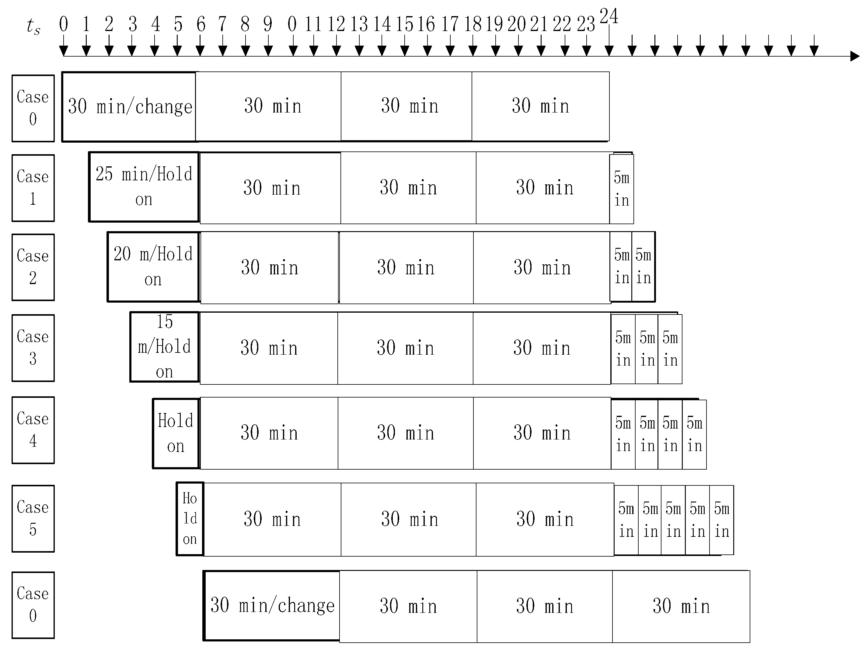
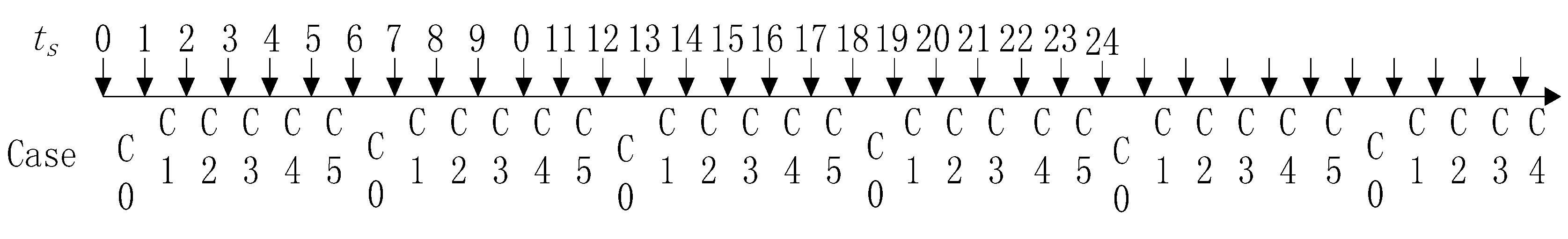
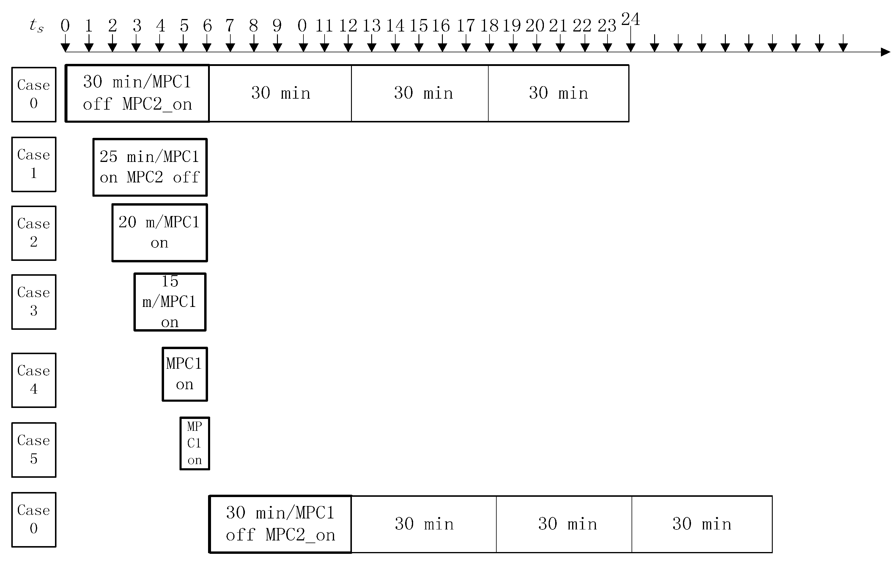
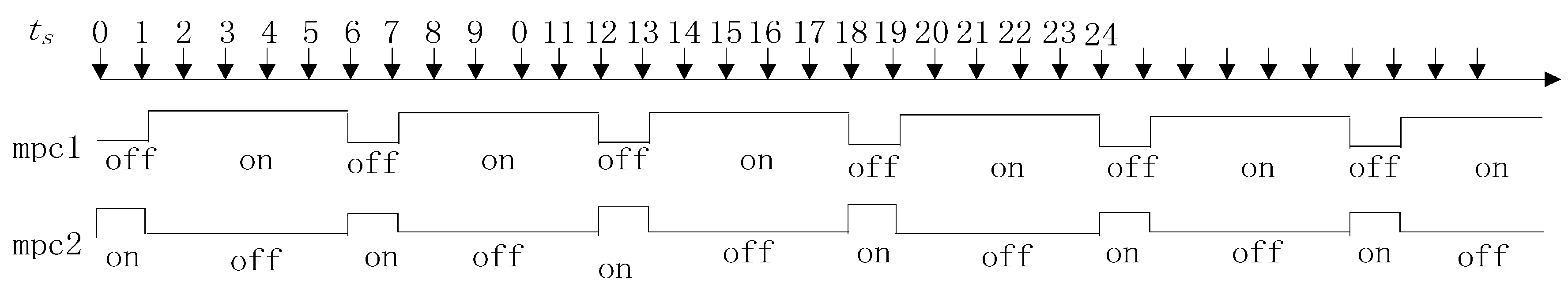
4.3. Two-Level Rolling Optimization

As mentioned in Section 3.2, a hierarchical MPC is adopted to present the system considered in this study. MPC 1 mainly controls the fly wheel, and MPC 2 mainly manages the pumped hydro storage. In contrast, the single-level MPC manages both the pumped hydro storage and the fly wheel. The pumped hydro storage system and one of the MPC controllers are regarded as the outer level, and the fly wheel storage system and the other MPC controller are regarded as the inner level. The outer level and inner level run alternatively to perform real-time scheduling. First, the outer level runs for one scheduling interval for optimization and then stops, thus obtaining long term scheduling results and sending some results to the inner level as input. Next, the inner level performs a short-term scheduling task. For a real-time scheduling system, the solution speed is one of the important system characteristics. In Figure 7, for Case 0, the control horizon is two hours, and the two-hour period is useful for pumped storage because pumped storage mainly addresses the slow fluctuation. To obtain the slow fluctuation by decomposing the wind power, this relatively long control horizon is essential. However, because the flywheel mainly manages turbulence fluctuations, the two hour period is unnecessary for the following reasons: (1) the turbulence fluctuation is difficult to forecast, i.e., the accuracy decreases with an increase in the prediction horizon; and (2) the solution time increases with an increase in the prediction horizon. We reduce the prediction horizon when the fly wheel is used. In other words, the prediction horizon of the fly wheel (MPC 1) decreases significantly, and the prediction horizon of the pumped hydro storage (MPC 2) remains unchanged. The reduction of the fly wheel (MPC 1) prediction horizon is performed in the two-level rolling optimization, as shown in Figure 7.

From Figure 7, it can be noted that at the beginning of scheduling (Case 0), MPC 2, which manages the pumped hydro storage, is on and MPC 1 is off. The MPC2 controller makes decisions based on the two-hour prediction horizon. The decisions include a key one that is the decision of pumped storage. The pumped storage decision is transmitted to the inner MPC (MPC 1) as an input value. In Cases 1–5, the pumped storage value is a constant, not a decision variable at the initial time. Moreover, the prediction of MPC1 is 25, 20, 15, 10, 5 min for the different cases for the above reasons.

Figure 7. Two-level MPC performing rolling optimization.

Figure 7. Two-level MPC performing rolling optimization.

Let t_s be equal to 0, corresponding to the time when the system is set into operation. The two-level rolling optimization process is presented as follows:

First (Step 1), when t_s = 0, the condition is Case 0. Only the MPC 2 controller is available, and the MPC 1 does not make system decisions. The MPC 2 controller obtains information, which is similar to that of the single-level approach; next, MPC 2 makes optimal decisions and then performs these decisions. In addition, the pumped hydro storage operating state is then transferred to the MPC 1 controller. The main purpose of the first step is to carry out a long-term and a look-ahead dispatch when the system begins to work. Because the optimal results contain some of the future information, the results can indicate the tendency of current values. The long-term rolling optimization is used to conduct the macro meteorological fluctuations by controlling the pumped storage. In Step 1, the pumped storage obtains an optimal result, and in case 0, the pumped storage in under control. We can use the following equation to describe the under control pumped storage.

$$\text{Case}0:p_t^{\text{px}}=p_{t+1}^{\text{px}}=p_{t+2}^{\text{px}}=p_{t+3}^{\text{px}}=p_{t+4}^{\text{px}}=p_{t+5}^{\text{px}}(t=0,6,12,18)$$

(22)

The Equation (22) describes that the pumped storage must keep the work state unchanged for half an hour, and the specific optimal value is decided by the optimal model. Therefore, in case 0, the pumped storage is under control. Meanwhile Equation (22) also shows that the prediction horizon is two hours, and it is a long-term optimization.

Second (Step 2), when t_s = 1, the condition is Case 1. MPC 2 does not make system decisions, and MPC 1 takes charge of making decisions. The MPC 1 controller obtains information (except for the pumped hydro storage information). MPC 1 then makes optimal decisions (except for pumped hydro storage decisions) and performs actions based on the decisions. Note that the MPC 1 controller cannot be in charge of the pumped hydro storage. The main purpose of the second step is to carry out a short-term and a look-ahead dispatch when the system continues to work. The short-term rolling optimization is used to deal with the turbulences by controlling the fly wheel. In Case 1, the pumped storage participated in scheduling; however, the power value of pumped storage was not decided in Case 1, and it is up to Case 0. In Case 1, the decision process of the pumped storage can be described by the following equation:

$$\text{Case}1:p_{t=0}^{\text{px}}=p_{t=1}^{\text{px}}=p_{t=2}^{\text{px}}=p_{t=3}^{\text{px}}=p_{t=4}^{\text{px}}=p_{t\_initial}^{\text{px}}$$

(23)

where $p_{t\_initial}^{\text{px}}$ is the pumped hydro storage operating state at the beginning of the half-hour period.

$p_{t=0}^{\text{px}}=p_{t=1}^{\text{px}}=p_{t=2}^{\text{px}}=p_{t=3}^{\text{px}}=p_{t=4}^{\text{px}}=p_{t\_initial}^{\text{px}}$ means that, for this instance of rolling optimization, the pumped storage decision variable is constant at the initial time. In Equation (23), the prediction horizon is 25 min, this indicated that the computation burden is significant less than that of Case 0. This is main reason that two-level MPC is adopted to controlling wind farm and hybrid storages.

Third (Step 3), when t_s is in the range of 2–5, the conditions are Cases 2–5, respectively, and MPC 1 and MPC 2 operate as in Step 2.

Finally, when t_s = 6, a new 30 min period starts, and MPC1 and MPC 2 repeat Step 1 (Case 0). The relationship between t_s and the cases is expressed by Equation (1).

Figure 8 shows the work sequence of MPC1 and MPC2. In Figure 8, when t_s = 0, t_s = 6, t_s = 12…, a new 30 min period has arrived, and at these scheduling intervals, MPC 2 starts to work, while MPC 1 stops working. When t_s is in the range of 1–5, 7–11, …, MPC 2 stops working, and MPC 1 starts to work. Note that at any scheduling interval, only one MPC controller is working.

Figure 8. Collaboration diagram for MPC 1 and MPC 2.

Figure 8. Collaboration diagram for MPC 1 and MPC 2.

4.4. Two-Level MPC State-Space and Optimization Model

4.4.1. Two-level MPC state-space model

(a)

State-space of MPC 2

In Figure 7 Case 0, MPC 2 is working, while MPC 1 is not working. Case 0 is similar to Case 0 for the single-level MPC. Therefore, the state-space of the long-term MPC (MPC 1) can be represented by Equations (8) and (9).

(b)

State-space of MPC 1

In Cases 1–5, the pumped hydro storage must remain in its operating state at the initial time, and the decision value of the pumped hydro storage is constant. The sample dynastic equations are similar to Equations (4), (5), and (7), and the differences are the decision variables of the pumped hydro storage.

The equation for $p_t^{\text{ps}}$ is similar to Equation (7).

The fly wheel energy balance equation is similar to Equation (5).

The pumped hydro storage energy balance equation is similar to Equation (4).

Subsequently, the discrete-time three-order dynamic equation of the wind power with hybrid storages can be written as follows:

$$\begin{array}{l}X(k+1)=A\times X(k)+B_1\times u(k)+B_2\times \text{ε}(k)\\ \left(\begin{array}{l}{p_{k+1}}^{\text{ps}}\\ {E_{k+1}}^{\text{fw}}\\ {E_k}^{\text{ps}}\end{array}\right)=\left(\begin{array}{l}0 0 0\\ 0 1 0\\ 0 0 1\end{array}\right)\times \left(\begin{array}{l}{p_k}^{\text{ps}}\\ {E_k}^{\text{fw}}\\ {E_k}^{\text{ps}}\end{array}\right)+\left(\begin{array}{ccc}-1& -1& -1\\ {\text{η}}_3\Delta t& \frac{-\Delta t}{{\text{η}}_4}& 0\\ 0& 0& 0\end{array}\right)\times \left(\begin{array}{l}{p}_k^{\text{fa}}\\ p_k^{\text{fp}}\\ p_k^{\text{wu}}\end{array}\right)+\left(\begin{array}{lll}1& -1& -1\\ 0& 0& 0\\ 0& {\text{η}}_{\text{1}}\Delta t& \frac{-\Delta t}{{\text{η}}_{\text{2}}}\end{array}\right)\times \left(\begin{array}{l}{p}_k^{\text{wind}}\\ p_k^{\text{pa}}\\ p_k^{\text{pp}}\end{array}\right)\end{array}$$

(24)

and the output equation is:

$$\begin{array}{l}y(k)=C\times X(k)\\ {p_k}^{\text{ps}}=\left(1 0 0\right)\times \left(\begin{array}{l}{p_k}^{\text{ps}}\\ {E_k}^{\text{fw}}\\ {E_k}^{\text{ps}}\end{array}\right)\end{array}$$

(25)

4.4.2. Two-Level MPC Programming Model

(a)

Programming Model of MPC2

The programming model of MPC2 is similar to that of single-level MPC Case 0; therefore, the objection and constraints can be represented by Equations (10)–(16).

(b)

Programming Model of MPC1

MPC 1 addresses Cases 1–5. In these cases, the pumped hydro storage variable is a constant.

(1)

MPC1 Objective Function of the Model

$$\min {\displaystyle \sum _{t=0}^N}\left(w_1\left|{p_t}^{\text{sp}}-{p_t}^{\text{plan}}\right|+w_2{p_t}^{\text{wu}}-w_3{p_t}^{\text{wd}}\right)$$

(26)

(2)

MPC1 Constraints

Equations (11)–(15) are also the constraints of MPC 1 because the prediction horizon is reduced significantly, i.e., it is smaller than that of the single-level MPC, as described in Table 2.

Table 2. Parameters for different cases of two-level model predictive control (MPC1).

Parameter	Case 0	Case 1	Case 2	Case 3	Case 4		Case 5
N	23	4	3	2		1	0
t	0–23	0–4	0–3	0–2		0–1	0
$p_t^{\text{px}}$	variable	Constant	Constant	Constant		Constant	constant

Table 2. Parameters for different cases of two-level model predictive control (MPC1).

Parameter	Case 0	Case 1	Case 2	Case 3	Case 4		Case 5
N	23	4	3	2		1	0
t	0–23	0–4	0–3	0–2		0–1	0
$p_t^{\text{px}}$	variable	Constant	Constant	Constant		Constant	constant

The MPC1 constraints of Assumption 1 are presented as follows:

$$\text{Case}1:p_{t=0}^{\text{px}}=p_{t=1}^{\text{px}}=p_{t=2}^{\text{px}}=p_{t=3}^{\text{px}}=p_{t=4}^{\text{px}}=p_{t\_initial}^{\text{px}}$$

(27)

$$\text{Case}2:p_{t=0}^{\text{px}}=p_{t=1}^{\text{px}}=p_{t=2}^{\text{px}}=p_{t=3}^{\text{px}}=p_{t\_initial}^{\text{px}}$$

(28)

$$\text{Case}3:p_{t=0}^{\text{px}}=p_{t=1}^{\text{px}}=p_{t=2}^{\text{px}}=p_{t\_initial}^{\text{px}}$$

(29)

$$\text{Case}4:p_{t=0}^{\text{px}}=p_{t=1}^{\text{px}}=p_{t\_initial}^{\text{px}}$$

(30)

$$\text{Case}5:p_{t=0}^{\text{px}}=p_{t\_initial}^{\text{px}}$$

(31)

The meanings of the five constraints are the same as those in Equation (17).

5. Simulation Results and Discussion

To verify the proposed scheduling method, extensive simulations are performed based on an actual wind farm using MATLAB (R2011a) and Cplex (12.4) software. The data used in this study are obtained from the power generation data for a wind farm in Inner Mongolia, China, with an installed capacity of 50 MW. The sampling time of the MPC is 5 min. The simulations have a duration of 24 h and include a total of 288 test points in total. At each sampling point, the forecast power data of the wind farm is required, and these data can be obtained from the prediction software or algorithm [36]. In this paper, these data are obtained by adding random noise to the power data of a real wind farm. The parameters of pumped storage and flywheel storage are listed in Table 3.

The parameters of the hybrid storage systems are taken from our previous study [37]. In [33], we considered the minimized investment and the maximized revenue of hybrid storage systems. A wind farm power dataset covering a one-year timespan is used to obtain the optimal storage.

Table 3. Parameter representations of the pumped storage station and the fly wheel power station.

Type	Charging Power (MW)	Discharging Power (MW)	Initial Energy (MWh)	Minute Energy (MWh)	Maximum Energy (MWh)	Efficiency (η1, η2)	Efficiency (η3, η4)
Pumped storage	100	100	100	20	200	0.87	0.85
Fly wheel	10	10	2.5	0.0	5	0.95	0.95

Table 3. Parameter representations of the pumped storage station and the fly wheel power station.

Type	Charging Power (MW)	Discharging Power (MW)	Initial Energy (MWh)	Minute Energy (MWh)	Maximum Energy (MWh)	Efficiency (η1, η2)	Efficiency (η3, η4)
Pumped storage	100	100	100	20	200	0.87	0.85
Fly wheel	10	10	2.5	0.0	5	0.95	0.95

The aim of this research was to present two MPC models to manage a wind farm and a hybrid storage system. In Section 5.1, the simulation results of the single-level MPC are compared with those of the two-level MPC.

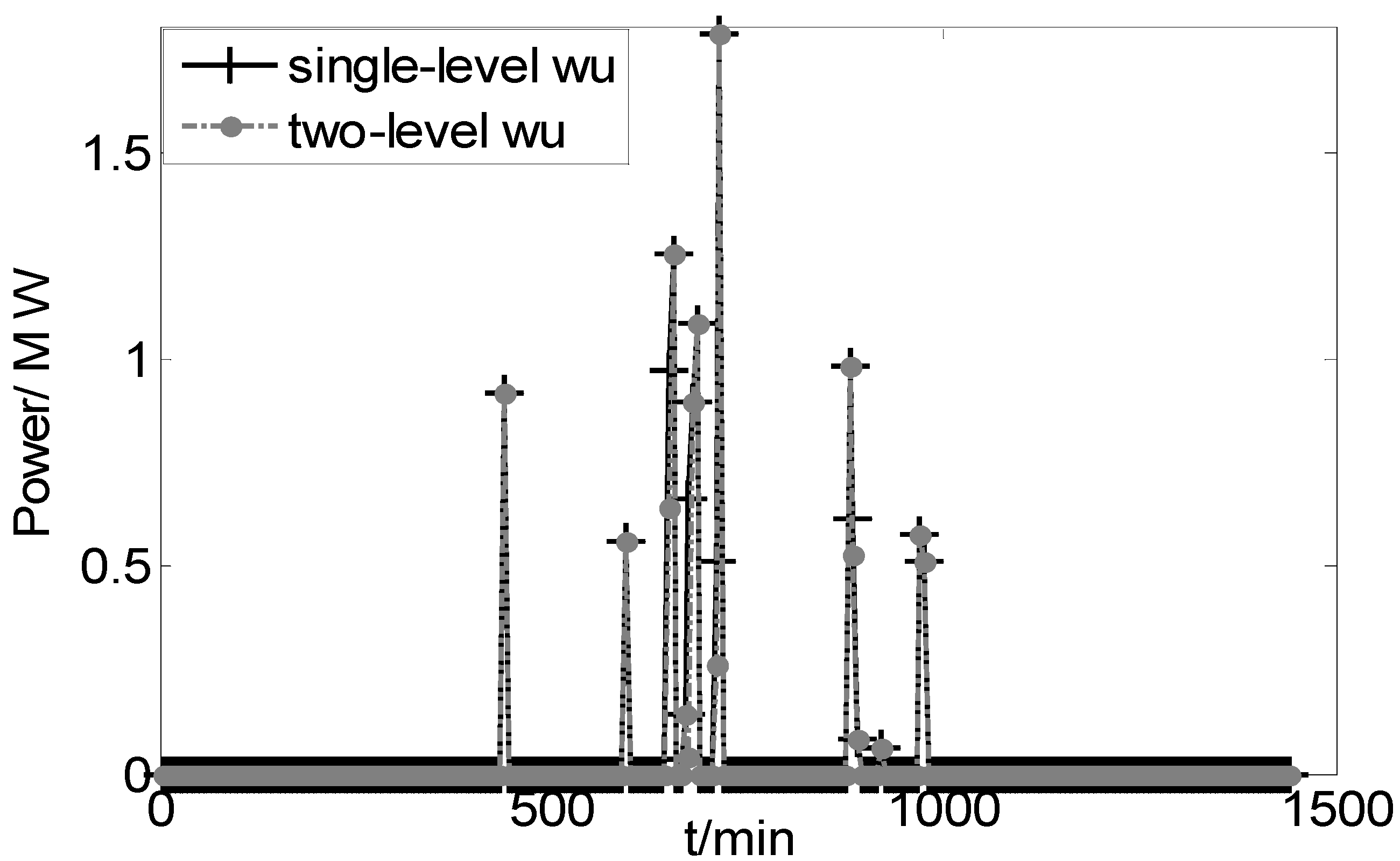
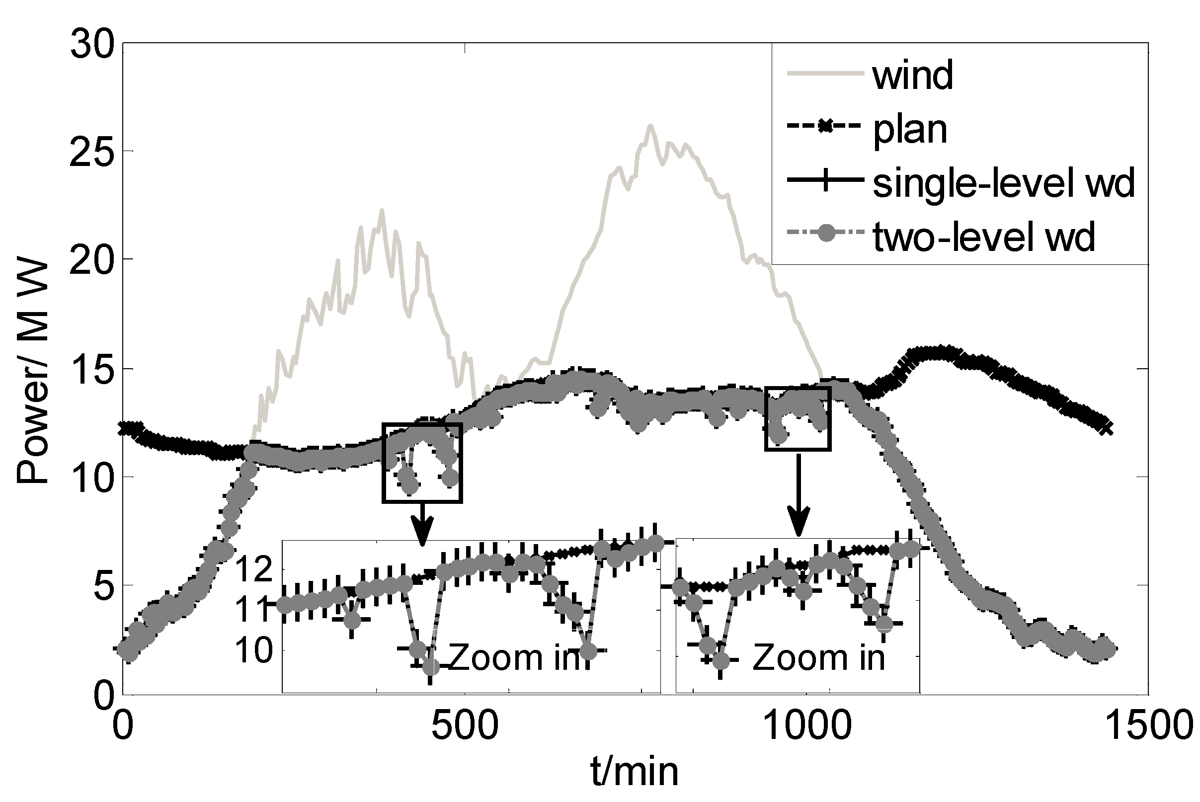
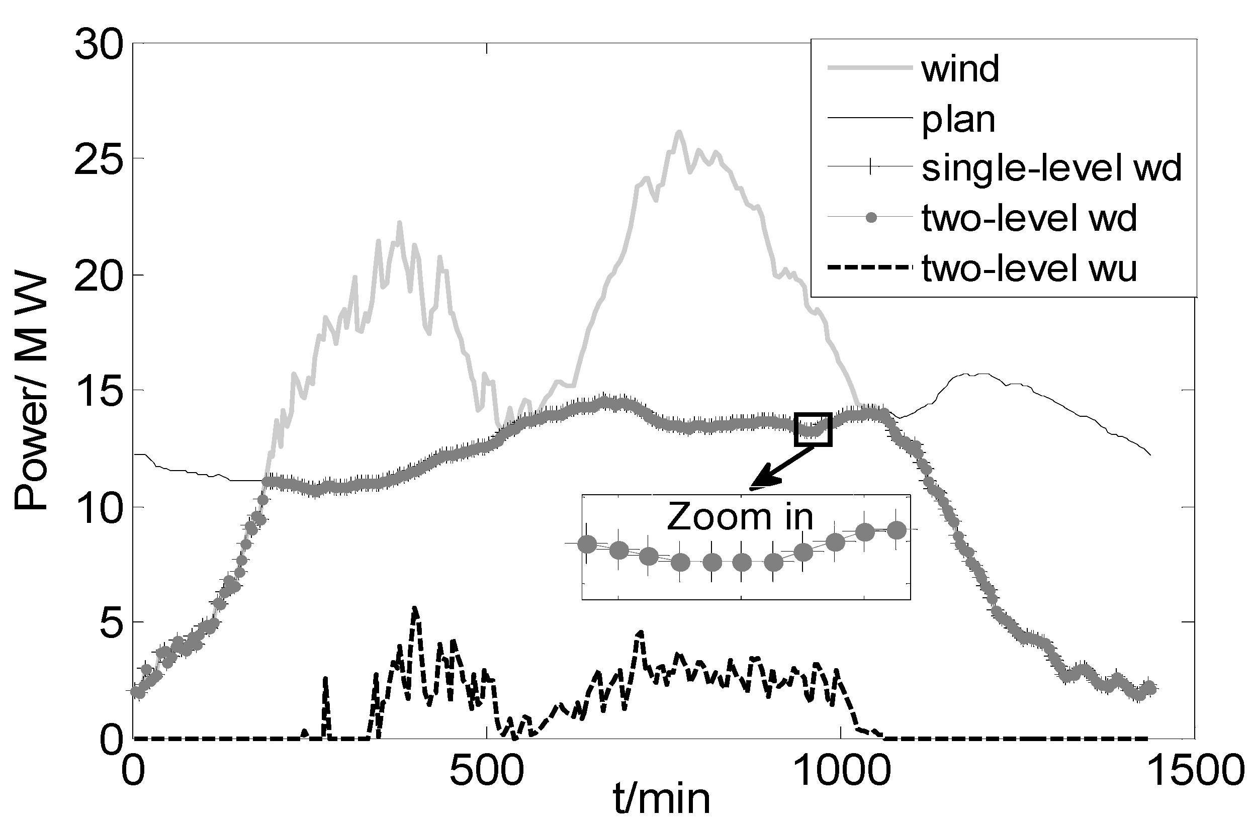
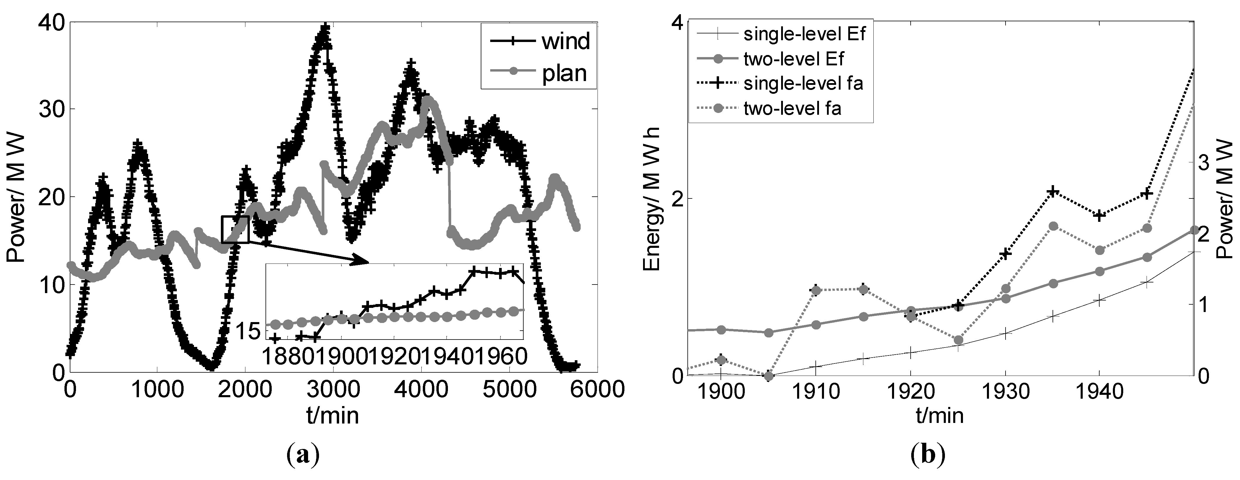
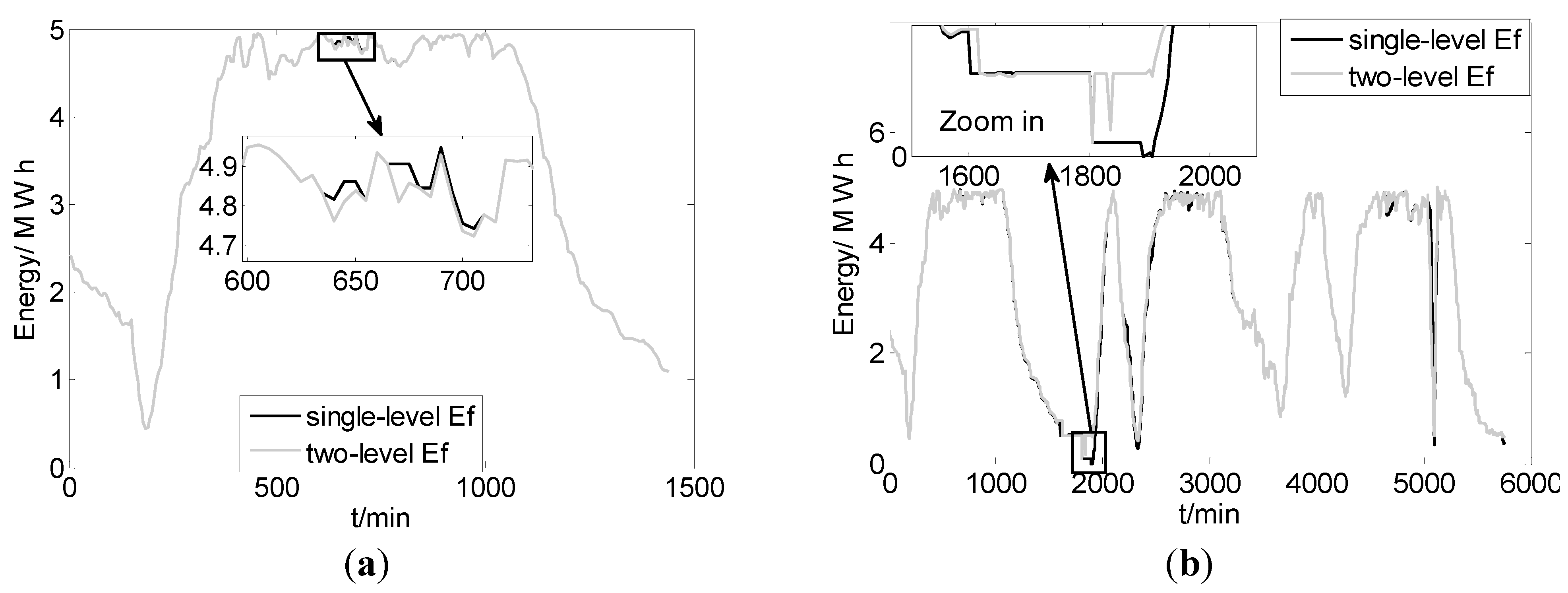
5.1. Simulation Test for Three Sub-Objectives Based on Single-Level and Two-Level MPC

Three sub-objectives were tested under the condition that w₁ = 0.9, w₂ = 1.0, and w₃ = 0.1, where w₁, w₂, and w₃ are the weighting coefficients of three sub-objectives. Note that in Section 5.1, the weighting coefficients are constants; however, in Section 5.2, the values of these coefficients vary with time.

Figure 9 shows the time histories of the power signals over the 24 h simulation time. Three power signals are shown: the plan power of the grid plan (solid, red), the single-level generation power of the wind-storage system ${p_t}^{\text{ps}}$ (dash-plus, black), and the two-level generation power of the wind-storage system ${p_t}^{\text{ps}}$ (dash-dot, gray).

From Figure 9, it can be noted that the single-level ps follows the plan closely, except for some points. From the magnified views of different areas, ps clearly does not follow the plan clearly at 655, 680 or 710 min. Two possible reasons for the differences between the single-level ps and plan are as follows: (1) the capacity of fly wheel storage is close to saturation in these moments, strongly limiting the charging ability, and (2) the weight of wind curtailment (w₂ = 1.0) is greater than that of the difference between ps and plan (w₁ = 0.9). It seems that a difference between the plan and ${p_t}^{\text{ps}}$ should be permitted, for reducing wind curtailment. Moreover, the two-level ps also follows the plan closely, except for the time points of 640, 655, 670, 680, 685, and 710. However, the two-level ps fails to follow the plan completely at the 880-minute point. It is likely that the single-level MPC method performed better than the two-level MPC method in terms of following the plan. A possible explanation for this behavior is that the prediction horizon of the single-level MPC is longer than that of the two-level MPC, as shown in Figure 5 and Figure 7.

Figure 9. Simulation result for the first sub-objective.

Figure 9. Simulation result for the first sub-objective.

The two-level MPC method has the benefit of reducing the solution time. For the two-level method, the average computing time of a scheduling interval is approximately 12.1 ms, while for the single-level MPC method, the time is 33.6 ms. In other words, the two-level method significantly reduces the computing time by approximately 64%.

The result of the second sub-objective is as follows.

In Figure 10, two power signals are depicted: the single-level wind curtailment (wu) (solid-plus, black) and the two-level wind curtailment (dash-dot, gray). Figure 10 shows the results of the wind curtailment of the single-level MPC method vs. that of the two-level MPC method. For both methods, the time of occurrence of wind curtailment is nearly the same, and the amount of single-level wu is approximately the same as that of the two-level wu. The amount of single-level wu is 11.68 MW, corresponding to 0.3% wind energy during a day, while that of two-level wu is 10.35 MW, corresponding to 0.26% wind energy. The results suggest that for the second sub-objective, the two-level MPC method may be slightly better than the single-level MPC method.

This waste of wind-sourced energy can be attributed to two main reasons: (a) the fly wheel is almost full, and (b) although the pumped hydro storage has a large amount of unused storage, it is constrained by Assumption 1, which does not allow it to use the excess wind energy.

Taking the single-level MPC as an example, the following explains the reason for the first wind curtailment. As shown in Figure 10, the first wind curtailment occurs at minute 435 (interval 88), t_s = 88. From Equation (1), we know that pumped hydro storage is in Case 4, i.e., it remained unchanged from 420 to 445 min (six scheduling intervals, half hour). Some basic information is provided as follows.

Figure 10. Simulation result for the second sub-objective.

Figure 10. Simulation result for the second sub-objective.

Table 4 indicates that the wind power is greater than the grid plan ($p_t^{\text{wind}}>p_t^{\text{plan}}$), and the excess wind energy must be stored in the storage systems. In Equation (4) ($p_t^{\text{wind}}=p_t^{\text{wd}}+p_t^{\text{pa}}+p_t^{\text{fa}}+p_t^{\text{wu}}$), $p_t^{\text{wind}}$ is 20.15 MW; $p_t^{\text{wd}}$ is 12.18 MW, due to the third sub-objective and constraints (Equation (17)); $p_t^{\text{pa}}$ is assigned as 6.39 MW according to assumption 1. Based on Equation (7) and ${E_{t+1}}^{\text{fw}}=5.0\text{MW}\cdot \text{h}$, ${E_t}^{\text{fw}}=4.809\text{MW}\cdot \text{h}$, we can calculate $p_t^{\text{fa}}$ as 0.66 MW. Finally, based on Equation (4) and the above results ($p_t^{\text{wind}}$,$p_t^{\text{wd}}$,$p_t^{\text{pa}}$,$p_t^{\text{fa}}$), we can calculate $p_t^{\text{wu}}$ as 0.93 MW.

Table 4. Analysis on the cause of the wind curtailment.

Values	Time(min)
	435	440	445	450	455
$p_t^{\text{plan}}$ /MW	12.18	12.19	12.20	12.21	12.26
$p_t^{\text{wind}}$ /MW	20.15	20.16	16.26	18.45	17.39
$p_t^{\text{wd}}$ /MW	12.18	12.19	9.86	12.21	12.26
$p_t^{\text{pa}}$ /MW	6.39	6.39	6.39	4.51	4.51
$p_t^{\text{fp}}$ /MW	0.66	2.42	0	1.73	0.62
$E_t^{ps}$ /MW·h	98.58	99.03	99.48	99.80	100.1
$E_t^{\text{fw}}$ /MW·h	4.809	5.0	4.80	4.93	4.98

Table 4. Analysis on the cause of the wind curtailment.

Values	Time(min)
	435	440	445	450	455
$p_t^{\text{plan}}$ /MW	12.18	12.19	12.20	12.21	12.26
$p_t^{\text{wind}}$ /MW	20.15	20.16	16.26	18.45	17.39
$p_t^{\text{wd}}$ /MW	12.18	12.19	9.86	12.21	12.26
$p_t^{\text{pa}}$ /MW	6.39	6.39	6.39	4.51	4.51
$p_t^{\text{fp}}$ /MW	0.66	2.42	0	1.73	0.62
$E_t^{ps}$ /MW·h	98.58	99.03	99.48	99.80	100.1
$E_t^{\text{fw}}$ /MW·h	4.809	5.0	4.80	4.93	4.98

The result of the third sub-objective is shown as follows:

Figure 11 shows the wind power that is directly sent to the grid $p_t^{\text{wd}}$ (wd). Moreover, Figure 11 shows that the single-level $p_t^{\text{wd}}$ is equal to the two-level $p_t^{\text{wd}}$. The reason for this may be as follows: $p_t^{\text{wd}}$ is the third sub-objective. When $p_t^{\text{wind}}<p_t^{\text{plan}}$ (the inequality means the wind power is less than the grid demand; thus, the storage systems must release energy to compensate for the missing energy between the wind power and the grid demand—in other words, in this situation, $p_t^{\text{pa}},p_t^{\text{fa}},p_t^{\text{wu}}$ are equal to 0), to maximize $p_t^{\text{wd}}$, and meet the constraint $p_t^{\text{wind}}=p_t^{\text{wd}}+p_t^{\text{pa}}+p_t^{\text{fa}}+p_t^{\text{wu}}$, $p_t^{\text{wind}}$ should be equal to $p_t^{\text{wd}}$. Therefore, when $p_t^{\text{wind}}<p_t^{\text{plan}}$, the single-level $p_t^{\text{wd}}$ is equal to $p_t^{\text{wind}}$, and the two-level wd is equal to $p_t^{\text{wind}}$. Therefore, the single-level $p_t^{\text{wd}}$ is equal to the two-level $p_t^{\text{wd}}$.

Figure 11. Simulation result for the third sub-objective.

Figure 11. Simulation result for the third sub-objective.

In contrast, when $p_t^{\text{wind}}>p_t^{\text{plan}}$, to maximize $p_t^{\text{wd}}$ while meeting the constraint $p_t^{\text{wind}}=p_t^{\text{wd}}+p_t^{\text{pa}}+p_t^{\text{fa}}+p_t^{\text{wu}}$ and $p_t^{\text{wd}}\le p_t^{\text{plan}}$, the optimal $p_t^{\text{wd}}$ should be equal to $p_t^{\text{plan}}$. However, when the fly wheel is almost full, wind curtailments ($p_t^{\text{wu}}$) will occur. We know that the $p_t^{\text{wu}}$ weighting coefficient w₂ (w₂ = 1.0) is larger than the $p_t^{\text{wd}}$ weighting coefficient w₃ (w₃ = 0.1), and the difference between w₂ and w₃ forms a decision principle; that is, for reducing wind curtailments, sacrificing $p_t^{\text{wd}}$ is permitted. Therefore, as shown in Figure 11, when $p_t^{\text{wind}}>p_t^{\text{plan}}$, $p_t^{\text{wd}}$ are equal to $p_t^{\text{plan}}$, except for some scheduling intervals in which $p_t^{\text{wd}}<p_t^{\text{plan}}$. From the above analysis, we remark that there was a significant possibility of the single-level $p_t^{\text{wd}}$ being equal to the two-level $p_t^{\text{wd}}$. Moreover, exchanging w₂ and w₃ yields the following results.

After exchanging w₂ and w₃, the $p_t^{\text{wu}}$ weighting coefficient w₂ (w₂ = 0.1) is less than the $p_t^{\text{wd}}$ weighting coefficient w₃ (w₃ = 1.0), and the new decision principle for maximizing $p_t^{\text{wd}}$, i.e., sacrificing wind curtailments ($p_t^{\text{wu}}$), is permitted. Therefore, $p_t^{\text{wd}}$ is equal to $p_t^{plan}$, and the wind curtailments ($p_t^{\text{wu}}$) increase greatly when $p_t^{\text{wind}}>p_t^{\text{plan}}$. In other words, the single-level $p_t^{\text{wd}}$ is equal to the two-level $p_t^{\text{wd}}$. Although exchanging w₂ and w₃ is infeasible, this result implies that $p_t^{\text{wd}}$ is influenced by the sub-objective, Equation (17), w₂ and w₃.

From the above-mentioned information, for the third sub-objective, the effect of the single-level MPC method is equal to that of the two-level MPC method.

The operating states of pumped storage are as follows:

Figure 13 shows the one-day and four-day test results for pumped storage; from Figure 13a, it can be seen that the ${E_t}^{\text{ps}}$ (Ep) of the single-level MPC method is equal to that of the two-level MPC method. To show the differences between the single-level and the two-level MPC, one-day simulations were performed, and the results are depicted in Figure 13b. As shown in the figure, the values of ${E_t}^{\text{ps}}$ for the two cases are equal, except at some points. For example, at minute 1920, the two ${E_t}^{\text{ps}}$ values begin to differ. Moreover, the two $p_t^{\text{pa}}$ (pa) values also start to display differences. A possible explanation for these differences between the pairs of ${E_t}^{\text{ps}}$ and $p_t^{\text{pa}}$ values is as follows:

Figure 12. Simulation result for the third sub-objective after the exchange of w₂ and w₃.

Figure 12. Simulation result for the third sub-objective after the exchange of w₂ and w₃.

Figure 13. Operating states of pumped storage. (a) one day states of the pumped storage; (b) four days states of the pumped storage.

Figure 13. Operating states of pumped storage. (a) one day states of the pumped storage; (b) four days states of the pumped storage.

In Figure 14a, from minute 1060 to minute 1900, $p_t^{\text{wind}}<p_t^{\text{plan}}$, i.e., during the period (1060–1900), the storage systems must release energy to the grid. Both single-level ${E_t}^{\text{ps}}$ (Ep) and two-level ${E_t}^{\text{ps}}$ (Ep) decrease rapidly to 20 MWh (minimized pumped storage capacity). Further, from Figure 14b, the fly wheel capacity decreases to zero MWh (minimized fly wheel capacity). At Minute 1905, $p_t^{\text{wind}}>p_t^{\text{plan}}$, i.e., the storage systems can store excess energy. At minute 1920, the two-level MPC method is in Case 0 (Equation (1)); in Case 0, the model of the two-level MPC method is similar to that of the single-level MPC method. Meanwhile, the pumped storage of the two-level MPC method is 20 MWh, and the wind power and plan is also equal. The only difference is the capacity of the fly wheel. As shown in Figure 14b, at minute 1920, the fly wheel capacity of the single-level MPC is 0.26 MWh, and that of the two-level MPC is 0.73 MWh; their difference leads to the difference in the pumped storage. A sensitivity analysis was performed for the capacity of the fly wheel and $p_t^{\text{pa}}$ of the pumped storage; and the result is described below.

As shown in Figure 15, the curve of $p_t^{\text{pa}}$ is a steep curve, indicating that $p_t^{\text{pa}}$ is not sensitive to the capacity of the fly wheel. In other words, the decision for the pumped storage is not closely related to the capacity of the fly wheel. This observation explains why the pumped storage operating state of the single-level MPC method is always similar to that of the two-level MPC method.

Figure 14. Minute 1920 of the wind power plan and operating states of the fly wheel. (a) Four days wind power and plan; (b) Operating states of the fly wheel.

Figure 14. Minute 1920 of the wind power plan and operating states of the fly wheel. (a) Four days wind power and plan; (b) Operating states of the fly wheel.

Figure 15. Sensitivity analysis for the capacity of the fly wheel and $p_t^{\text{pa}}$ of the pumped storage.

Figure 15. Sensitivity analysis for the capacity of the fly wheel and $p_t^{\text{pa}}$ of the pumped storage.

Figure 16 shows the one-day and four-day operating states of the fly wheel. The differences for the fly wheel are greater than those for the pumped storage, and the differences for former often occurs when the fly wheel is nearly full or empty. The differences may be attributed to the length of the prediction horizon. In the single-level MPC method, the length is two hours, while it is less than half an hour in the two-level MPC method.

Figure 16. Operating states of the fly wheel. (a) One day operating states of fly wheel; (b) Four days operating states of fly wheel.

Figure 16. Operating states of the fly wheel. (a) One day operating states of fly wheel; (b) Four days operating states of fly wheel.

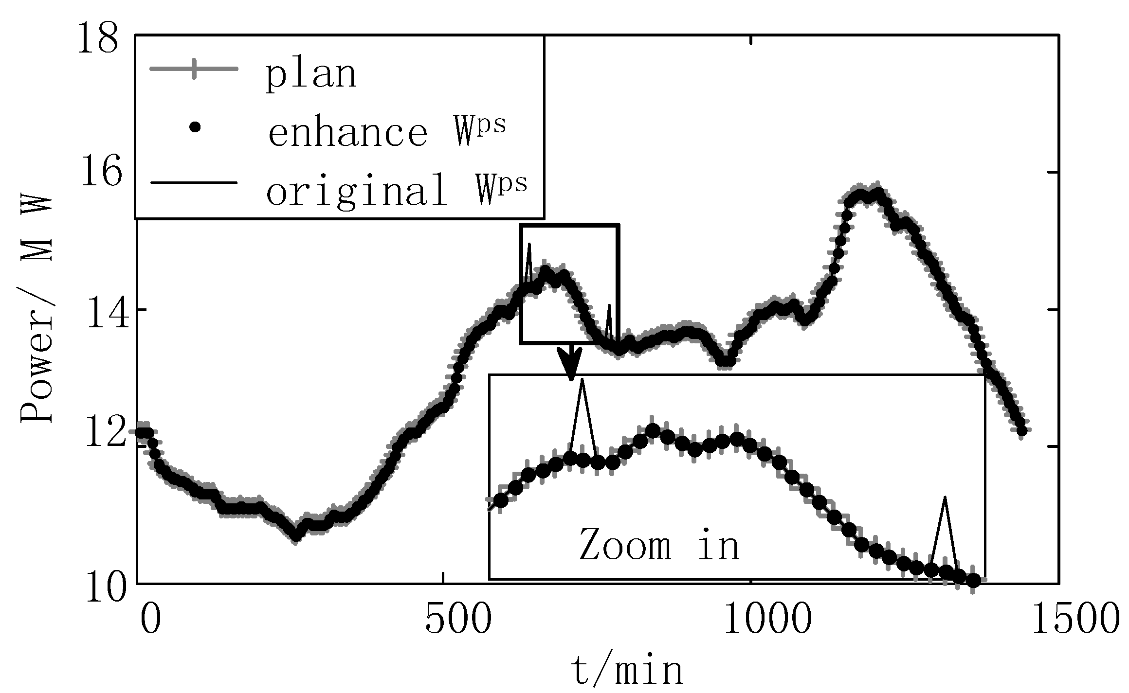
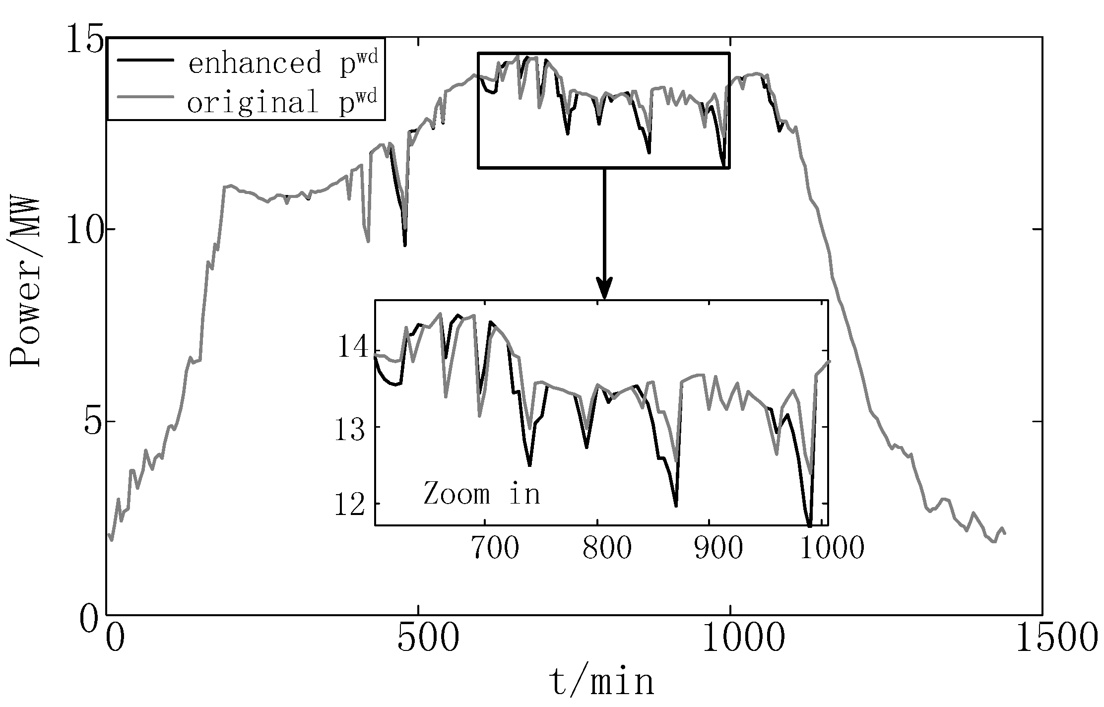
5.2. Simulation Test for Strengthening the Weighting Coefficients of the First Scheduling Interval

In the MPC decision process, only the current time decision values are determined, and the future (the remainder) decision values are discarded. Due to this difference in processing, we consider that the weights of the current time decision values should be greater than those of the future decision values. The simulation test validates our hypothesis. Although this idea is simple, it is an effective means of improving the optimal objective. For the sake of the simplicity of the simulation test, only the single-level MPC method was used to test this hypothesis. The test is described as follows:

The first weighting coefficients were increased by a factor of five, and the rest remained unchanged. The expressions for the weighting coefficients are:

$$w_1(t)=\left\{\begin{array}{l}2.5t=1\\ 0.5t=\mathrm{2...},24\end{array}\right\},w_2(t)\text{=}\left\{\begin{array}{l}0.5t=1\\ 0.1t=\mathrm{2...},24\end{array}\right\},w_3(t)\text{=}\left\{\begin{array}{l}5.0t=1\\ 1.0t=\mathrm{2...},24\end{array}\right\}$$

(32)

The system was simulated for a 24 h period. The results of three sub-objectives are as follows:

Figure 17 shows the comparison of $p_t^{\text{ps}}$ using the increased and original weights, respectively. In Figure 17, three power signals are shown: the plan of the grid $p_t^{\text{plan}}$ (solid, gray), the enhanced weight $p_t^{\text{ps}}$ (no line-dot, black), and the original weight $p_t^{\text{ps}}$ (line, black). The enhanced weight $p_t^{\text{ps}}$ follows the plan of the grid completely, whereas, for the original weight $p_t^{\text{ps}}$, a slight error is observed. This result suggests that the method of increasing the weight could assist $p_t^{\text{ps}}$ in tracing the plan of the grid.

Figure 18 shows the comparison result of $p_t^{\text{wu}}$ using the enhanced weight and the original weight, respectively. In Figure 18, four power signals are shown: the plan of the grid $p_t^{\text{plan}}$ (solid-plus, red), the available wind power $p_t^{\text{wind}}$ (dash, gray), the enhanced weight of wind curtailment $p_t^{\text{wu}}$ (solid, black), and the original weight of wind curtailment $p_t^{\text{wu}}$ (solid, gray). Note that there are two y-axes: the origin of the left y-axis is zero, and $p_t^{\text{plan}}$, $p_t^{\text{wind}}$, and the enhanced weight of wind curtailment $p_t^{\text{wu}}$ are correlated; Moreover, the origin of the right y-axis is −2, and it is a correlation of the original weight of wind curtailment $p_t^{\text{wu}}$. The two y-axes are set to different scales and intercepts to prevent the overlap of the two $p_t^{\text{wu}}$. As the weight of first moment increases, the number of times $p_t^{\text{wu}}$ occurred and decreases from 17 to 12, and $p_t^{\text{wu}}$ decreases from 0.974 to 0.915 MWh. Comparing the two $p_t^{\text{wu}}$, we can find the enhanced weight $p_t^{\text{wu}}$ occurs for five fewer times, and the amount of the enhances weight decreased by 6%.

Figure 17. Results of the first objective after increasing the weighting.

Figure 17. Results of the first objective after increasing the weighting.

Figure 18. Simulation results for the second objective after strengthening the weight.

Figure 18. Simulation results for the second objective after strengthening the weight.

To show the details of the reduction of $p_t^{\text{wu}}$, the case of the minute 435 was tested again with the same data. For the original weight of $p_t^{\text{wu}}$, reduction occurs at minute 435, while for the enhanced weight of $p_t^{\text{wu}}$, it does not occur. The decision values obtained are listed in Table 5.

Table 5. Case analysis of the increased weights.

Values	Time (min)
	435	440	445	450	455
$p_t^{\text{plan}}$/MW	12.18	12.19	12.20	12.21	12.26
$p_t^{\text{wind}}$/MW	20.15	20.16	16.26	18.45	17.39
$p_t^{\text{pa}}$/MW	6.39	6.39	6.39	4.51	4.51
$p_t^{\text{fa}}$/MW	1.581	1.507	0	1.729	0.619
$p_t^{\text{fp}}$/MWh	0	0	2.34	0	0
$p_t^{\text{wd}}$/MW	12.18	12.19	9.86	12.21	12.26
$E_t^{\text{ps}}$/MW·h	98.58	99.03	99.48	99.80	100.1
$E_t^{\text{fw}}$/MW·h	4.881	5.0	4.80	4.98	4.89
$p_t^{\text{wu}}$/MW	0	0.917	0	0	0

Table 5. Case analysis of the increased weights.

Values	Time (min)
	435	440	445	450	455
$p_t^{\text{plan}}$/MW	12.18	12.19	12.20	12.21	12.26
$p_t^{\text{wind}}$/MW	20.15	20.16	16.26	18.45	17.39
$p_t^{\text{pa}}$/MW	6.39	6.39	6.39	4.51	4.51
$p_t^{\text{fa}}$/MW	1.581	1.507	0	1.729	0.619
$p_t^{\text{fp}}$/MWh	0	0	2.34	0	0
$p_t^{\text{wd}}$/MW	12.18	12.19	9.86	12.21	12.26
$E_t^{\text{ps}}$/MW·h	98.58	99.03	99.48	99.80	100.1
$E_t^{\text{fw}}$/MW·h	4.881	5.0	4.80	4.98	4.89
$p_t^{\text{wu}}$/MW	0	0.917	0	0	0

Table 5 shows the MPC decision result for the enhanced weight. Note that for this test, minute 435 is the current time, and minutes 440–455 are future times. Comparing Table 5 with Table 4, we find that only the amounts of $p_t^{\text{fa}}$, $p_t^{\text{fp}}$ and $E_t^{\text{fw}}$ change. From Table 5, the wind curtailment does not occur at the current moment (minute 435) but shifts to a future time (minute 440). According to the MPC decision process, the current time decision value is used, while the rest of the decision values are discarded. Moreover, when the next scheduling times arrive, the MPC makes decisions, and the result for minute 440 does not exhibit wind curtailment. Therefore, at minute 435, all the wind energy is utilized, without any waste.

The results suggested that the method of enhancing weight could assist the MPC in reducing the number of times of occurrence and the amount of wind curtailment.

Figure 19 shows the comparison result of $p_t^{\text{wd}}$ using for the enhanced and original weights respectively. In Figure 19, two power signals are shown: the enhanced weight of $p_t^{\text{wd}}$ (solid, black) and the original weight of $p_t^{\text{wd}}$ (solid, gray). Figure 19 shows that when wind < plan, both $p_t^{\text{wd}}$ values are basically equal to wind, while both $p_t^{\text{wd}}$ values are very close to plan when wind > plan. Therefore, the third objective is achieved. However, the comparison result shows that the enhanced weight $p_t^{\text{wd}}$ is slightly less than the original weight $p_t^{\text{wd}}$. One possible explanation for this result is that $p_t^{\text{wd}}$ is sacrificed to reduce the wind curtailment $p_t^{\text{wu}}$.

Figure 19. Simulation results for the third objective after increasing the weight.

Figure 19. Simulation results for the third objective after increasing the weight.

6. Conclusions

This paper presented two real-time MPC scheduling models that utilize storage systems to assist the wind farm in meeting the scheduling of the grid. On the basis of the different control constructions, the models are classified a single-level MPC model and a two-level MPC model. Both models have their own advantages, and they cannot be interchanged. The single-level MPC runs steadily and has a high capability to follow the plan of the grid. In contrast, the two-level MPC provides high calculation speed, and the optimal objectives are close to those of the single-level MPC. Moreover, the decision values of the pumped storage are not sensitive to the fly wheel capacity and that, in some situations, the wind power generation sent to the grid ( $p_t^{\text{wd}}$ ) is sacrificed to reduce the wind curtailment. In addition, the method of weight enhancement is simple, practical, and can be easily implemented in real-time applications.

Further research is required to consider the operational stability of the two-level MPC and reduce the number of times of fly wheel charging and discharging.

References

1. Breton, S.P.; Moe, G. Status, plans and technologies for offshore wind turbines in Europe and North America. Renew. Energy 2009, 34, 646–654. [Google Scholar] [CrossRef]
2. Zhang, H.; Gao, F.; Wu, J. Optimal bidding strategies for wind power producers in the day-ahead electricity market. Energies 2012, 5, 4804–4823. [Google Scholar] [CrossRef]
3. Teleke, S.; Baran, M.E.; Huang, A.Q. Control strategies for battery energy storage for wind farm dispatching. IEEE Trans. Energy Convers. 2009, 24, 725–732. [Google Scholar] [CrossRef]
4. Wang, X.Y.; Mahinda Vilathgamuwa, D.; Choi, S.S. Determination of battery storage capacity in energy buffer for wind farm. IEEE Trans. Energy Convers. 2008, 23, 868–878. [Google Scholar] [CrossRef]
5. Khalid, M.; Savkin, A.V. Model predictive control for wind power generation smoothing with controlled battery storage. In Proceedings of the 2009 Joint 48th IEEE Conference on Decision and Control (CDC) and 28th Chinese Control Conference (CCC 2009), Shanghai, China, 15–18 December 2009; pp. 7849–7853.
6. Yi, Z.; Songzhe, Z.; Chowdhury, A.A. Reliability modeling and control schemes of composite energy storage and wind generation system with adequate transmission upgrades. IEEE Trans. Sustain. Energy 2011, 2, 520–526. [Google Scholar]
7. Khatamianfar, A.; Khalid, M.; Savkin, A.V. Wind power dispatch control with battery energy storage using model predictive control. In Procedings of the 2012 IEEE International Conference on Control Applications (CCA), Dubrovnik, Croatia, 3–5 October 2012; pp. 733–738.
8. DufoLópez, R.; BernalAgustín, J.L.; DomínguezNavarro, J.A. Generation management using batteries in wind farms: Economical and technical analysis for spain. Energy Policy 2009, 37, 126–139. [Google Scholar] [CrossRef]
9. Chao, G.; Ye, Z.; Hao, Z. Optimal Storage Sizing for Composite Energy Storage and Wind in Micro Grid. In Proceedings of the 2014 14th International Conference on Environment and Electrical Engineering (EEEIC), Krakow, Poland, 10–12 May 2014; pp. 286–290.
10. Duong, T.; Haihua, Z.; Khambadkone, A.M. Energy management and dynamic control in composite energy storage system for micro-grid applications. In Proceedings of the IECON 2010—36th Annual Conference on IEEE Industrial Electronics Society, Glendale, AZ, USA, 7–10 November 2010; pp. 1818–1824.
11. Wang, Z.; Li, G.; Li, G.; Yue, H. Studies of multi-type composite energy storage for the photovoltaic generation system in a micro-grid. In Proceedings of the 2011 4th International Conference on Electric Utility Deregulation and Restructuring and Power Technologies (DRPT), Weihai, China, 6–9 July 2011; pp. 791–796.
12. Abbey, C.; Strunz, K.; Joos, G. A knowledge-based approach for control of two-level energy storage for wind energy systems. IEEE Trans. Energy Convers. 2009, 24, 539–547. [Google Scholar] [CrossRef]
13. Wang, B.; Zhang, B.; hao, Z. Control of composite energy storage system in wind and pv hybrid microgrid. In Proceedings of the 2013 IEEE International Conference of IEEE Region 10 (TENCON 2013), Xian, China, 22–25 October 2013; pp. 1–5.
14. Tan, X.; Wang, H.; Li, Q. Multi-port topology for composite energy storage and its control strategy in micro-grid. In Proceedings of the 2012 7th International Power Electronics and Motion Control Conference (IPEMC), Harbin, China, 2–5 June 2012; pp. 351–355.
15. Zadeh, A.K.; Abdel-Akher, M.; Wang, M.; Senjyu, T. Optimized day-ahead hydrothermal wind energy systems scheduling using parallel pso. In Proceedings of the 2012 International Conference on Renewable Energy Research and Applications (ICRERA), Nagasaki, Janpan, 11–14 November 2012; pp. 1–6.
16. Marzband, M.; Sumper, A.; Ruiz-Alvarez, A. Experimental evaluation of a real time energy management system for stand-alone microgrids in day-ahead markets. Appl. Energy 2013, 106, 365–376. [Google Scholar] [CrossRef]
17. Marzband, M.; Ghadimi, M.; Sumper, A. Experimental validation of a real-time energy management system using multi-period gravitational search algorithm for microgrids in islanded mode. Appl. Energy 2014, 128, 164–174. [Google Scholar] [CrossRef] [Green Version]
18. Kassem, A.M.; Zaid, S.A. Load parameter waveforms improvement of a stand-alone wind-based energy storage system and takagi-sugeno fuzzy logic algorithm. IET Renew. Power Gener. 2014, 8, 775–785. [Google Scholar] [CrossRef]
19. Romaus, C.; Gathmann, K.; Bo, X.; Cker, J. Optimal energy management for a hybrid energy storage system for electric vehicles based on stochastic dynamic programming. In Proceedings of the Vehicle Power and Propulsion Conference (VPPC), Lille, France, 1–3 September 2010; pp. 1–6.
20. Marzband, M.; Sumper, A.; Dominguez-Garcia, J.; Gumara-Ferret, R. Experimental validation of a real time energy management system for microgrids in islanded mode using a local day-ahead electricity market and minlp. Energy Convers. Manag. 2013, 76, 314–322. [Google Scholar] [CrossRef]
21. Qi, W.; Liu, J.; Christofides, P.D. Supervisory predictive control for long-term scheduling of an integrated wind/solar energy generation and water desalination system. IEEE Trans. Control Syst. Technol. 2012, 20, 504–512. [Google Scholar] [CrossRef]
22. Yonghao, G.; Chung, H.K.; Chung, C.C.; Yong-Cheol, K. Intra-day unit commitment for wind farm using model predictive control method. In Proceedings of the 2013 IEEE, UPower and Energy Society General Meeting (PES), Vancouver, BC, Canada, 21–25 July 2013; pp. 1–5.
23. Mayhorn, E.; Kalsi, K.; Elizondo, M.; Wei, Z.; Shuai, L.; Samaan, N.; Butler-Purry, K. Optimal control of distributed energy resources using model predictive control. In Proceedings of the 2012 IEEE Power and Energy Society General Meeting, San Diego, CA, USA, 22–26 July 2012; pp. 1–8.
24. Qi, W.; Liu, J.; Christofides, P.D. A two-time-scale framework to supervisory predictive control of an integrated wind/solar energy generation and water desalination system. In Proceedings of the American Control Conference (ACC), San Francisco, CA, USA, 29 June–1 July 2011; pp. 2677–2682.
25. Teleke, S.; Baran, M.E.; Bhattacharya, S.; Huang, A.Q. Optimal control of battery energy storage for wind farm dispatching. IEEE Trans. Energy Convers. 2010, 25, 787–794. [Google Scholar] [CrossRef]
26. Khalid, M.; Savkin, A.V. A model predictive control approach to the problem of wind power smoothing with controlled battery storage. Renew. Energy 2010, 35, 1520–1526. [Google Scholar] [CrossRef]
27. Xie, L.; Gu, Y.; Eskandari, A.; Ehsani, M. Fast mpc-based coordination of wind power and battery energy storage systems. J. Energy Eng. 2012, 138, 43–53. [Google Scholar] [CrossRef]
28. Khatamianfar, A.; Khalid, M.; Savkin, A.V.; Agelidis, V.G. Improving wind farm dispatch in the australian electricity market with battery energy storage using model predictive control. IEEE Trans. Sustain. Energy 2013, 4, 745–755. [Google Scholar] [CrossRef]
29. Scattolini, R. Architectures for distributed and hierarchical model predictive control—A review. J. Process Control 2009, 19, 723–731. [Google Scholar] [CrossRef]
30. Westermann, D.; Nicolai, S.; Bretschneider, P. Energy management for distribution networks with storage systems—A hierarchical approach. In Proceedings of the Power and Energy Society General Meeting—Conversion and Delivery of Electrical Energy in the 21st Century, Pittsburgh, PA, USA, 20–24 July 2008; pp. 1–6.
31. Kennel, F.; Gorges, D.; Liu, S. Energy management for smart grids with electric vehicles based on hierarchical mpc. IEEE Trans. Ind. Inf. 2013, 9, 1528–1537. [Google Scholar] [CrossRef]
32. Li, K.; Xu, H.; Ma, Q.; Zhao, J. Hierarchy control of power quality for wind—Battery energy storage system. IET Power Electron. 2014, 7, 2123–2132. [Google Scholar] [CrossRef]
33. Zhang, L.; Li, Y. Optimal energy management of wind-battery hybrid power system with two-scale dynamic programming. IEEE Trans. Sustain. Energy 2013, 4, 765–773. [Google Scholar] [CrossRef]
34. Paatero, J.V.; Lund, P.D. Effect of energy storage on variations in wind power. Wind Energy Wiley 2005, 8, 421–441. [Google Scholar] [CrossRef]
35. Feng, G.; Hallam, A.; Chien-Ning, Y. Wind generation scheduling with pump storage unit by collocation method. In Proceedings of the 2099. PES’09. IEEE Power & Energy Society General Meeting, Calgary, AB, Canada, 26–30 July 2009; pp. 1–8.
36. Marzband, M.; Azarinejadian, F.; Savaghebi, M.; Guerrero, J.M. An optimal energy management system for islanded microgrids based on multiperiod artificial bee colony combined with markov chain. IEEE Syst. J. 2015. [Google Scholar] [CrossRef]
37. Meng, X.; Feng, G.; Zhang, H. Optimization design for hybrid energy storage device in wind farm taking scheduling into account. Power Syst. Technol. 2014, 38, 1853–1860. [Google Scholar]