Photovoltaic Electricity for Sustainable Building. Efficiency and Energy Cost Reduction for Isolated DC Microgrid

Abstract

In the context of sustainable buildings, this paper investigates power flow management for an isolated DC microgrid and focuses on efficiency and energy cost reduction by optimal scheduling. Aiming at high efficiency, the local produced power has to be used where, when, and how it is generated. Thus, based on photovoltaic sources, storage, and a biofuel generator, the proposed DC microgrid is coupled with the DC distribution network of the building. The DC bus distribution maximizes the efficiency of the overall production-consumption system by avoiding some energy conversion losses and absence of reactive power. The isolated DC microgrid aims to minimize the total energy cost and thus, based on forecasting data, a cost function is formulated. Using a mixed integer linear programming optimization, the optimal power flow scheduling is obtained which leads to an optimization-based strategy for real-time power balancing. Three experimental tests, operated under different meteorological conditions, validate the feasibility of the proposed control and demonstrate the problem formulation of minimizing total energy cost.

1. Introduction

Currently, some major preoccupations in urban area are the buildings energy performances and energy autonomy. Nowadays, in urban areas, there is a significant development of small plants of decentralized photovoltaic (PV) power production, therefore associated with or integrated in buildings [1,2]. Facing high PV sources penetration level in future, direct PV power injection may introduce additional regulations in grid power balancing, resulting in power quality or even stability issues. Therefore, microgrids are proposed as a key integration of renewable energy in the grid power energy mix [3]. By grouping production, consumption and storage together, the microgrid operates in grid-connected and off-grid modes. In grid-connected operating mode, a microgrid can exchange power with the grid (to receive or to inject power). During off-grid operating mode, a microgrid should be able to continuously provide enough energy to an important part of its internal load. AC or DC microgrids combine power balancing control and energy management in order to control on-site generation and power demand [4]. Despite existing researches on microgrid power balancing [5,6], local power optimization for building-integrated DC microgrid [7,8,9,10] has not been fully explored.

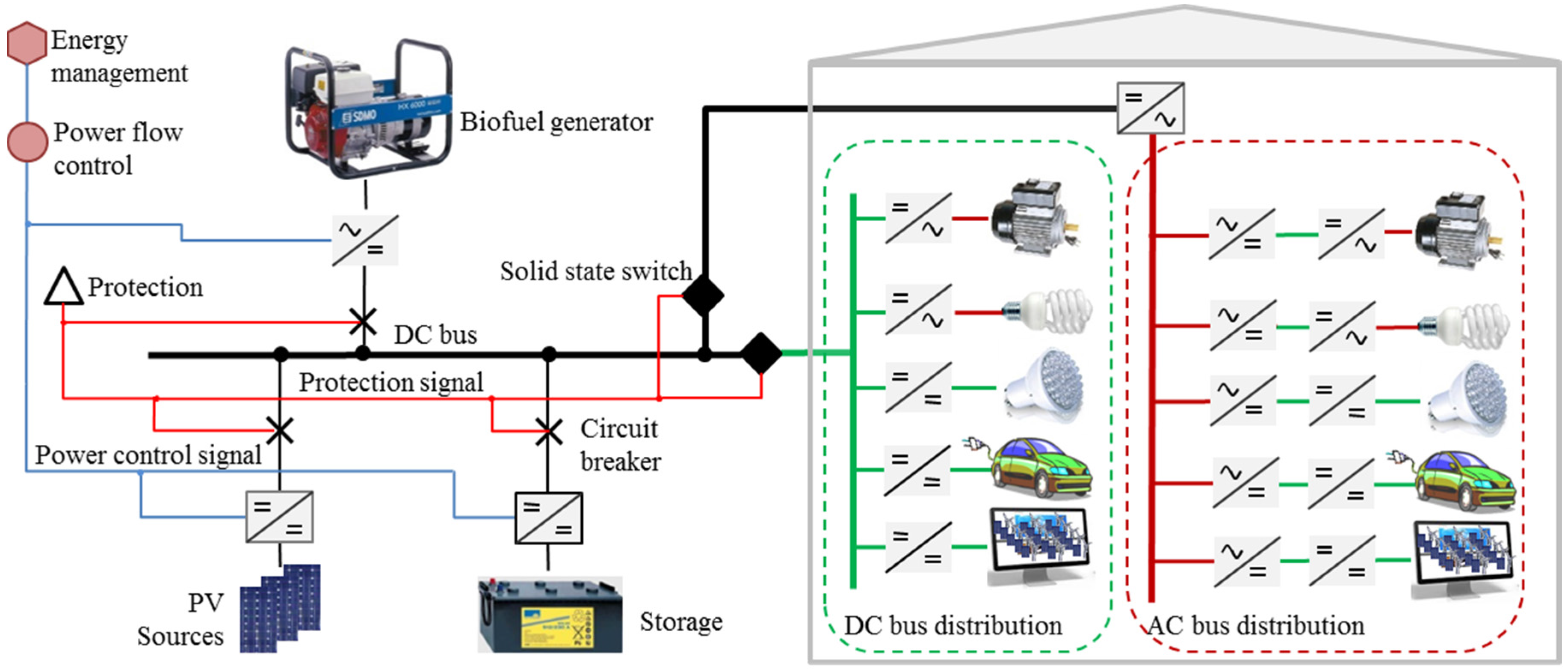
In this context, facing the emergence of the smart grid combined with AC or DC microgrids, on the one hand, and the increasing of the positive-energy buildings, on the other hand, one of the solutions is the local DC microgrid based on PV sources that are the most commonly used renewable sources in urban area. This paper presents an isolated DC microgrid with optimized power flow for improving PV penetration and positive-energy buildings. As concerns the building-integrated DC microgrid [9,10,11], it is possible to design a DC power distribution in an energy efficient manner because most of its electric loads operate directly with DC power [12]. Protection devices, such as solid-state circuit and hybrid breakers, are nowadays technically feasible, in accordance with the specification of breaking time and perturbation on the bus [13].

The goal is to design an advanced local energy management and control, which optimizes power flow for improving PV efficiency for positive-energy buildings. Specifically, for buildings equipped with PV sources, this study presents an isolated DC microgrid which handles instantaneous power balancing following an optimal power flow scheduling while providing energy cost reduction. The optimization takes into account forecast of PV power production and load power demand, while satisfying constraints such as storage capability and sources operating modes [14,15]. Optimization, wherein efficiency is related to the prediction accuracy, may be carried out by several methods: linear and direct methods, meta-heuristic algorithms, rule-based methods, etc. [16,17,18]. In [17] three optimization methods were chosen to solve an optimal power flow scheduling: mixed integer linear programming as a direct method that has guarantees of convergence, differential evolution as a meta-heuristic that is not limited to linear problems or constraints, and rule-based algorithm as a quick and fast method for a particular case. The goal was to optimize the use of the resources and to minimize the total energy cost. Following this comparison, the rule-based algorithm was arguably the fastest, but with increased complexity of the PV sources power forecasted curve, the efficiency of this rule-based algorithm has dropped considerably. The mixed integer linear programming had the best tradeoff between computational duration and accuracy, performing the optimization in less time than the differential evolution that depends on calculating many generations to reach the result.

This paper investigates power flow management for an isolated DC microgrid and focuses on efficiency and energy cost reduction by optimal scheduling. Based on PV sources, storage, and biofuel generator, the proposed DC microgrid is described in Section 2. The power management and optimization are presented in Section 3. Combined with robust power balance strategy, the optimization is able to minimize the total energy cost. Section 4 gives experimental results and validates the feasibility of implementing optimization in real operation while respecting rigid constraints. The experimental results are analyzed in Section 5. Conclusions are presented in Section 6.

2. Isolated Building-Integrated DC Microgrid

The building-integrated isolated DC microgrid is presented in Figure 1. PV sources, storage and biofuel generator are connected through their dedicated converters on a common DC bus. The common DC bus is chosen for an efficient integration of renewable sources and storage, and for the absence of frequency and phase synchronization; therefore only the DC bus voltage need to be stabilized [14].

Figure 1. Isolated DC microgrid based on photovoltaic (PV) sources, storage and biofuel generator.

Figure 1. Isolated DC microgrid based on photovoltaic (PV) sources, storage and biofuel generator.

The considered load is a set of electrical appliances of the building that are integrated in the DC microgrid; the load power which can be supplied depends on the microgrid power. The proposed microgrid is able to optimize the power flows at the bus to obtain a minimized daily cost for users [15] and a power control signal is transmitted to each converter.

2.1. DC Bus Distribution versus AC Bus Distribution

Figure 1 shows that the isolated DC microgrid can be connected to the electric building network either using an inverter at the output of the microgrid then to the AC bus distribution or considering a DC bus distribution directly connected to the DC bus of the microgrid.

Concerning the building electrical appliances, a great percentage of them could be fed directly with DC power, such as devices based on microprocessors, computer system power supply, switched-mode power supply, lighting based on LED and variable-frequency drives for the speed variation of the motors which equip the systems of heating, ventilation and air conditioning, lighting based on light emitting diodes [13].

The use of a DC network distribution has been already studied in many research works. Current trends given in [19] show that the power distribution networks are experiencing a transformation toward DC at both the generation and consumption level. Taking into account the growing use of electronic goods, electric vehicles, solid-state and electronically-driven lighting and motors, coupled with the increasing use of native DC renewable energy sources, in [9] the author presents the new electric energy network age as the “DC-empowered Enernet”. This system, based on buildings electric DC loads, is supplied by native DC distributed energy source. Regarding the voltage of DC bus distribution, in the case of a sustainable data center, it seems that 380V DC brings reliability and efficiency [20]. A low-voltage bipolar-type DC microgrid is proposed in [21]. The authors relate that this DC microgrid can supply super high quality power with three-wire DC distribution line for a residential complex. In [22], the performance of a supervisory control of an adaptive-droop regulated DC microgrid is assessed through experimental results. This methodology leads to a DC power system whose interest increases in renewable energy applications because of the good matching with DC output type sources. In [12] a DC distribution system for building loads is investigated. The DC power system is supplied by a DC distributed energy source for DC loads and has a separate AC grid connection for AC loads. These DC distribution systems for buildings lead to a higher efficiency compared to a system solely based on AC because of no need for rectifying. The authors note that power rectifiers have a relatively low efficiency compared to inverters and DC-DC converters. In [23], a study based on simulation has been carried out and the conclusion is that the power loss of DC microgrid is 15% less than that of AC microgrid.

To sum up, the DC bus distribution maximizes the efficiency of the overall production-consumption system by avoiding some energy conversion losses (elimination of one or two energy conversion stages) and absence of reactive power [24]. In addition, DC bus distribution is highly compatible with electricity storage which may increase the efficiency of plug-in hybrid electric vehicles and electric vehicles whose number is supposed to increase in a few years [25,26].

In traditional AC bus distribution, the local microgrid produces DC power that is converted to AC power to supply building’s electric system; then, this power has to be re-converted to DC [9,12], for many end-devices as cited above and illustrated in Figure 1.

2.2. DC Microgrid Control Strategy

The DC microgrid coupled with a DC bus distribution is considered in this study. PV sources are mostly controlled by a maximum power point tracking (MPPT) algorithm [27], but could be controlled to output a limited power [28], if required. The storage system is an electrochemical system that is technically and economically well adapted for a building-integrated microgrid system. The storage is required to smooth the power output from renewable sources. The biofuel generator is used as back-up source and operates in bang-bang mode. In this study, the cogeneration aspect of the biofuel generator is not considered.

A set of building electrical appliances is supplied by a DC bus distribution; it forms the DC load, which consists of critical appliances and interruptible appliances. The critical appliances require a continuous power supply, while the interruptible appliances can be shed temporarily. The microgrid power control can send load shedding signal to disconnect some appliances; therefore, load power demand can only reach a limited power level denoted by $p_{L\_LIM}$. In order to describe this limit, a load shedding coefficient $K_L=p_{L\_LIM}/P_{L\_MAX}$ is defined, where $P_{L\_MAX}$ represents a constant value, which is the maximum of the load power and $K_L\in [0,1]$.

The microgrid power management and control are based on weather and load consumption short-term forecasting data. Using a PV sources model [29] and a load consumption model, they estimate PV sources power and load power. Based on these two prediction results, the microgrid optimizes the power flow while satisfying constraints. Thus, optimized predictive power flow is obtained and leads to calculate a control parameter $D$ which is a time varying value sequence. By applying $D$, as interface parameter, the power flow real-time control handles instantaneous power balancing with respect to constraints and ensures self-correcting capability [30].

The difference between load consumption and PV generation causes fluctuations in the DC bus voltage denoted by $v$. Thus, power balance is performed by adjusting storage and biofuel generator power for stabilizing $v$. The required power reference $p^{*}$ for power balancing is calculated by regulating $v$ with a proportional-integral controller as in Equation (1):

$$p^{*}=p_{PV}-p_L-C_P\left(v^{*}-v\right)-C_I{\displaystyle \int \left(v^{*}-v\right)dt}$$

(1)

where $p_{PV}$ is the PV sources power, $p_L$ is the load power, $v^{*}$ is DC bus constant voltage control reference, $C_P$ and $C_I$ are proportional and integral gain respectively. Then, $p^{*}$ is distributed to storage and biofuel generator in an optimized manner, according to control parameter $D$.

3. Power Management and Optimization

The isolated building-integrated DC microgrid has to supply the DC load while reducing global energy cost. The biofuel generator works in bang-bang mode, thus only the storage can be controlled continuously. Based on the power flow diagram shown in Figure 2, the following subsections present the microgrid power management and optimization.

Figure 2. Power flow diagram.

Figure 2. Power flow diagram.

3.1. Isolated DC Microgrid Control

As for all fuel generators based on thermal machine, due to low dynamic response, frequent start-stop cycles, and low output power, the biofuel generator efficiency is reduced and supplementary cost is introduced. To overcome these issues, in this study the biofuel generator is assigned with two operating states: off and output rated power given by Equation (2):

$$p_{BG}=k\cdot P_{BG\_P}\text{ with }k\in \{0,1\}$$

(2)

where $p_{BG}$ and $P_{BG\_P}$ are the biofuel generator power and biofuel generator rated power respectively. Considering a discrete time instant $t_i$, from initial $t_0$ to final $t_F$, with time interval $\Delta t$, a working duty cycle is assigned to biofuel generator control as in Equation (3):

$$\begin{array}{l}{p}_{BG}(t_i)=p_{BG}(t_{i-1})ifrem(t_i/d{t}_{BG})\ne 0\\ t_i=\{t_0+\Delta t,t_0+2\Delta t,\mathrm{\dots },t_F\}\end{array}$$

(3)

with $d{t}_{BG}$ the time duration of biofuel generator working duty cycle and rem the function that returns the remainder of the division. Since the biofuel generator works in duty cycle, it introduces the case that storage is charged by rated PV sources power plus rated biofuel generator power. As the high charging rate can largely affect the storage life, the storage power $p_S$ is limited as in Equation (4):

$$-P_{S\_MAX}\le p_S\le P_{S\_MAX}$$

(4)

with $P_{S\_MAX}$ the storage power limitation.

PV sources are supposed to operate with Perturb and Observe algorithm, as MPPT method [27], to produce MPPT power noted $p_{PV\_MPPT}$. Nevertheless, to protect storage from overcharging, the PV production may be partially shed by the limited PV production algorithm described in [28]. The PV sources power $p_{PV}$ is given by Equation (5):

$$p_{PV}=p_{PV\_MPPT}-p_{PV\_S}$$

(5)

where $p_{PV\_S}$ is the PV shed power whose values are calculated by optimization. In the MPPT operation algorithm $p_{PV\_S}=0$. As PV sources shedding should not induce negative power, PV sources power is constrained to $p_{PV}\ge 0$. If the storage state of charge, $soc$, does not reach its upper limit $SO{C}_{MAX}$, the PV production should not be limited, so $p_{PV\_S}=0\text{ if }soc<SO{C}_{MAX}$. When the storage is full or storage power could exceed its power limits, the PV sources power is limited to load power and is performed following as proposed and validated in [28].

The load power demand $p_{L\_D}$ should be satisfied according to end-user demand. To avoid or minimize the use of biofuel generator in case of insufficient storage and PV sources power, the load may be partially shed. The proportion in load power that must be shed is noted as $p_{L\_S}$, and the load power is calculated by Equation (6):

$$p_L=p_{L\_D}-p_{L\_S}$$

(6)

with $p_L$ the load power, with $p_L\ge 0$ and $0\le p_{L\_S}\le p_{L\_D}$. Load shedding occurs when storage reaches its lower limit $SO{C}_{MIN}$ or storage power could exceed power limits. In such cases, the load power is expected not to exceed $p_{L\_LIM}=p_{PV}+p_{BG}+P_{S\_MAX}$. If $soc>SO{C}_{MIN}$, then $p_{L\_S}=0$.

The storage is operated by current closed-loop control, and the storage power can be controlled by giving corresponding current reference. The $soc$ must be respected to its upper and lower limitations as described by Equation (7) and is calculated by Equation (8):

$$SO{C}_{MIN}\le soc\le SO{C}_{MAX}$$

(7)

$$soc=SO{C}_0+\frac{1}{v_S\cdot C_{REF}}{\displaystyle {\int }_{t_0}^t(p_{S\_C}}-p_{S\_D})dt$$

(8)

with $SO{C}_0$ as initial $soc$, $C_{REF}$ as storage nominal capacity (Ah), $v_S$ as storage voltage, and $p_S$ as storage power defined as $p_S=p_{S\_C}-p_{S\_D}$, where $p_{S\_C}$ and $p_{S\_D}$ are storage charging and discharging power respectively, which are both defined as positive number.

Considering that all powers are always positive by sign convention, power balancing is described by Equation (9):

$$p_{PV}+p_{BG}+p_{S\_D}=p_{S\_C}+p_L$$

(9)

3.2. Energy Cost Reduction by Optimization

Based on forecast of load power and forecast of PV sources power, the optimization goal is to obtain the best power distribution among the sources, so as to reduce energy cost, load shedding, PV sources shedding, and biofuel generator consumption. Therefore, microgrid power management and control minimizes the total energy cost $C_{total}$ as in Equation (10):

$$C_{total}=C_{BG}+C_S+C_{PVS}+C_{LS}$$

(10)

where $C_{BG}$ is the biofuel generator energy cost, $C_S$ is the storage energy cost, $C_{PVS}$ is the PV sources shedding cost, and $C_{LS}$ is the load shedding cost. By calculating the energy cost for each time duration $\Delta t$ and $t_i=\{t_0,t_0+\Delta t,t_0+2\Delta t,\mathrm{...},t_F\}$, these energy costs are defined by Equation (11):

$$\begin{array}{l}{C}_{BG}={\displaystyle \sum _{t_i=t_0}^{t_F}{c}_{BG}(t_i)\cdot \Delta t\cdot p_{BG}(t_i)}\\ C_S={\displaystyle \sum _{t_i=t_0}^{t_F}{c}_S(t_i)\cdot \Delta t\cdot (p_{S\_C}(t_i)}+p_{S\_D}(t_i))\\ C_{PVS}={\displaystyle \sum _{t_i=t_0}^{t_F}{c}_{PVS}(t_i)\cdot \Delta t\cdot p_{PV\_S}(t_i)}\\ C_{LS}={\displaystyle \sum _{t_i=t_0}^{t_F}{c}_{LS}(t_i)\cdot \Delta t\cdot p_{L\_S}(t_i)}\end{array}$$

(11)

with $c_{BG}$ the biofuel generator energy tariff, $c_S$ the storage energy tariff, $c_{PVS}$ the PV shedding energy tariff, $c_{LS}$ the load shedding energy tariff.

The PV sources power shedding and the load shedding are penalized by cost definition given by Equation (11). However, load shedding is not permitted when there is sufficient power supply, and PV sources shedding are not permitted when the production can be totally consumed. These constraints are implied in the optimization objective, and are also given in explicit form by Equation (12):

$$\begin{array}{l}\text{if }{p}_{PV\_MPPT}(t_i)>p_{L\_D}(t_i)\text{ then }{p}_{L\_S}(t_i)=0\\ \text{if }{p}_{PV\_MPPT}(t_i)=p_{L\_D}(t_i)\text{ then }\{\begin{array}{c}{p}_{L\_S}(t_i)=0\\ p_{PV\_S}(t_i)=0\end{array}\\ \text{if }{p}_{PV\_MPPT}(t_i)<p_{L\_D}(t_i)\text{ then }{p}_{PV\_S}(t_i)=0\end{array}$$

(12)

To ensure continuous operation, $soc$ lower limit at the end of one operation can also be assigned:

$$soc(t_F)\ge SO{C}_F$$

(13)

with $SO{C}_F$ a constant for the desired $soc$ value at final time.

As the optimization goal is to minimize biofuel consumption, to respect $soc$, to reduce load shedding and PV sources shedding, the optimization problem is formulated by Equation (14).

$$\begin{array}{l}\text{Minimize }{C}_{total}=C_{BG}+C_S+C_{PVS}+C_{LS}\\ \text{with respect to:}\\ \{\begin{array}{l}{p}_{PV}(t_i)+p_{BG}(t_i)+p_{S\_D}(t_i)=p_{S\_C}(t_i)+p_L(t_i)\\ p_S(t_i)=p_{S\_C}(t_i)-p_{S\_D}(t_i)\\ p_{PV}(t_i)=p_{PV\_MPPT}(t_i)-p_{PV\_S}(t_i)\\ p_L(t_i)=p_{L\_D}(t_i)-p_{L\_S}(t_i)\\ \text{if }{p}_{PV\_MPPT}(t_i)>p_{L\_D}(t_i)\text{ then }{p}_{L\_S}(t_i)=0\\ \text{if }{p}_{PV\_MPPT}(t_i)=p_{L\_D}(t_i)\text{ then }\{\begin{array}{c}{p}_{L\_S}(t_i)=0\\ p_{PV\_S}(t_i)=0\end{array}\\ \text{if }{p}_{PV\_MPPT}(t_i)<p_{L\_D}(t_i)\text{ then }{p}_{PV\_S}(t_i)=0\\ SO{C}_{MIN}\le soc(t_i)\le SO{C}_{MAX}\\ soc(t_i)=SO{C}_0+\frac{1}{v_S\cdot C_{REF}}{\displaystyle \sum _{t_i=t_0}^{t_F}{p}_S(t_i)}\Delta t\\ soc(t_F)\ge SO{C}_F\\ p_{PV}(t_i)\ge 0\\ p_L(t_i)\ge 0\\ p_{PV\_S}(t_i)\ge 0\\ p_{L\_S}(t_i)\ge 0\\ 0\le p_{BG}(t_i)\le P_{BG\_P}\\ -P_{S\_MAX}\le p_S(t_i)\le P_{S\_MAX}\\ p_{BG}(t_i)=k\cdot P_{BG\_P}\text{ with }k\in \{0,1\}\\ t_i=\{t_0,t_0+\Delta t,t_0+2\Delta t,\mathrm{\dots },t_F\}\end{array}\\ \{\begin{array}{l}{p}_{BG}(t_i)=p_{BG}(t_{i-1})ifrem(t_i/d{t}_{BG})\ne 0\\ t_i=\{t_0+\Delta t,t_0+2\Delta t,\mathrm{...},t_F\}\end{array}\end{array}$$

(14)

The optimization problem is formulated as a mixed integer linear programming problem [31], and solved by IBM ILOG CPLEX [32]. The energy management gives the optimized power flow as the time series evolution of $p_{S\_D}$, $p_{S\_C}$, $p_{BG}$, $p_L$, $p_{PV}$, which is translated to control parameter $D$ as interface energy management algorithm and power balancing control algorithm. As the biofuel generator is considered at two states, $D$ is defined as switching signal for biofuel generator operation, while storage power is assigned in control strategy to balance power. Thus, when $D=1$, biofuel generator starts and outputs the rated power; for $D=0$ biofuel generator has no specific order, therefore it is the power balancing control algorithm which determines to turn on or turn off the biofuel generator. The optimization result is presented in Section 4.

3.3. Power Balancing Control

The real-time power balancing, the control strategy should satisfy the following requirements: reproduce optimized power flow in real operating conditions while ensuring robustness and withstanding uncertainties introduced by forecasted powers. Biofuel generator works in bang-bang mode and only the storage power can be controlled continuously, which induces difficulty in power balancing due to the only one degree of freedom. As aforementioned, it could happen that the PV sources output rated power while the biofuel generator is turned on and load consumption is low. Charging storage with high power will shorten storage life, so, at least one source needs to be limited or cut-off. The priority is defined as shedding PV sources first, and then cut-off biofuel generator if SOC_MAX is reached. The power balancing control algorithm is illustrated in Figure 3.

Figure 3. Power balancing control algorithm.

Figure 3. Power balancing control algorithm.

Power balancing can be maintained with any value of $D$ between 0 and 1. Indeed, $D$ could be designed to take values between 0 and 1, representing a command for biofuel generator to output power under rated power. The power balancing control strategy is capable to operate with $D$ between 0 and 1. However, such action is not as economic as bang-bang mode and is thus not considered. In this paper, $D$ takes the value of either 0 or 1. Concerning self-correcting ability in power balancing, the biofuel generator power represents the most important degree of flexibility, but PV sources limited production and load shedding are also performed if necessary.

4. Experimental Tests of Isolated DC Microgrid Control

Table 1 gives the parameters used for optimization and power balancing control strategy.

Table 1. Optimization and experimental parameters values.

PBG_P	1500 W	CREF	130 Ah
dtBG	1200 s	SOCMIN	45%
PL_MAX	1700 W	SOCMAX	55%
v*	400 V	cBG	1.1 €/kWh
PS_MAX	1200 W	cS	0.01 €/kWh
PPV_MPPT at Standard Test Conditions	2000 W	cPVS	1 €/kWh
SOC0 = SOCF	50%	cLS	1 €/kWh

Table 1. Optimization and experimental parameters values.

PBG_P	1500 W	CREF	130 Ah
dtBG	1200 s	SOCMIN	45%
PL_MAX	1700 W	SOCMAX	55%
v*	400 V	cBG	1.1 €/kWh
PS_MAX	1200 W	cS	0.01 €/kWh
PPV_MPPT at Standard Test Conditions	2000 W	cPVS	1 €/kWh
SOC0 = SOCF	50%	cLS	1 €/kWh

These parameters are selected according to system configuration with an aim to involve as much system behavior as possible during the tests, such as storage events (full, empty), load shedding and PV sources power limiting. The energy tariffs values are chosen completely arbitrarily but in order to enhance the control strategy it is mandatory to respect the inequality c_BG > c_PVS(LS) >> c_S. Regarding DC bus voltage value which is the same as the DC bus distribution voltage value, in order to be economically profitable and to be able to use the already existing building cable infrastructure (400/230 V AC), research works show that an optimal value to adopt may be about 325 V DC [12]. For technical reasons, and after verification of the AC versus DC efficiency, in this study, the 400 V DC bus voltage is adopted.

The electrical scheme and images of experimental platform are presented in Figure 4 and Figure 5 respectively.

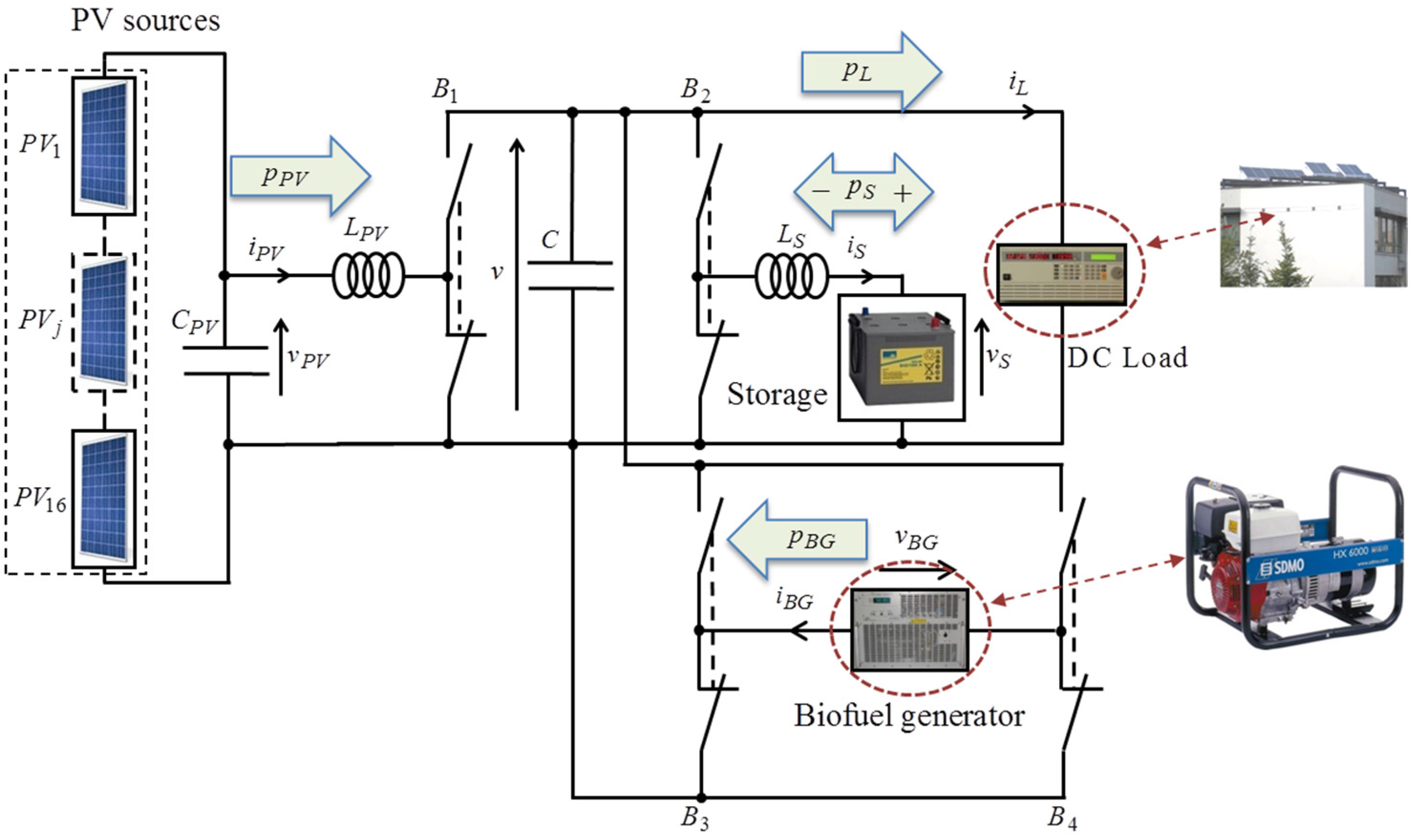
Figure 4. Electrical scheme of experimental platform.

Figure 4. Electrical scheme of experimental platform.

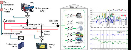
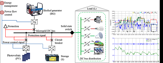
Figure 5. Test bench image.

Figure 5. Test bench image.

This experimental platform is installed in the laboratory of the research team EA 7284 AVENUES (Pierre Guillaumat Center of Universite de Technologie de Compiegne, France). The image of the DC load shows the PV panels on the roof of the Pierre Guillaumat Center. The biofuel generator and the DC load are emulated by a linear amplifier and a programmable DC electronic load respectively. In addition, a four-leg power converter (B₁ to B₄) and a set of inductors and capacitors, in order to ensure compatibility between the different elements, are added.

The control/optimization method was implemented in the experimental platform presented in Figure 5. Regarding the overall control structure, firstly, the simulation was implemented on MATLAB Simulink. To make it work in real time, it is compiled by dSPACE, and then the system operates using the ControlDesk from dSPACE real-time as a human-machine interface. Optimized results are power flows of each element (PV sources, storage, biofuel generator, and DC load), which are translated into $D$ to control the real operation. All controls are linear controls, operating with PI correctors, with PWM at 20 kHz. Finally, the PWM signals are routed to the driver cards which control independently the IGBT components. In order to simplify the control, in this study, all PI correctors are with disturbances compensation. Thus, note that the synthesis of PI correctors is not performed with high accuracy.

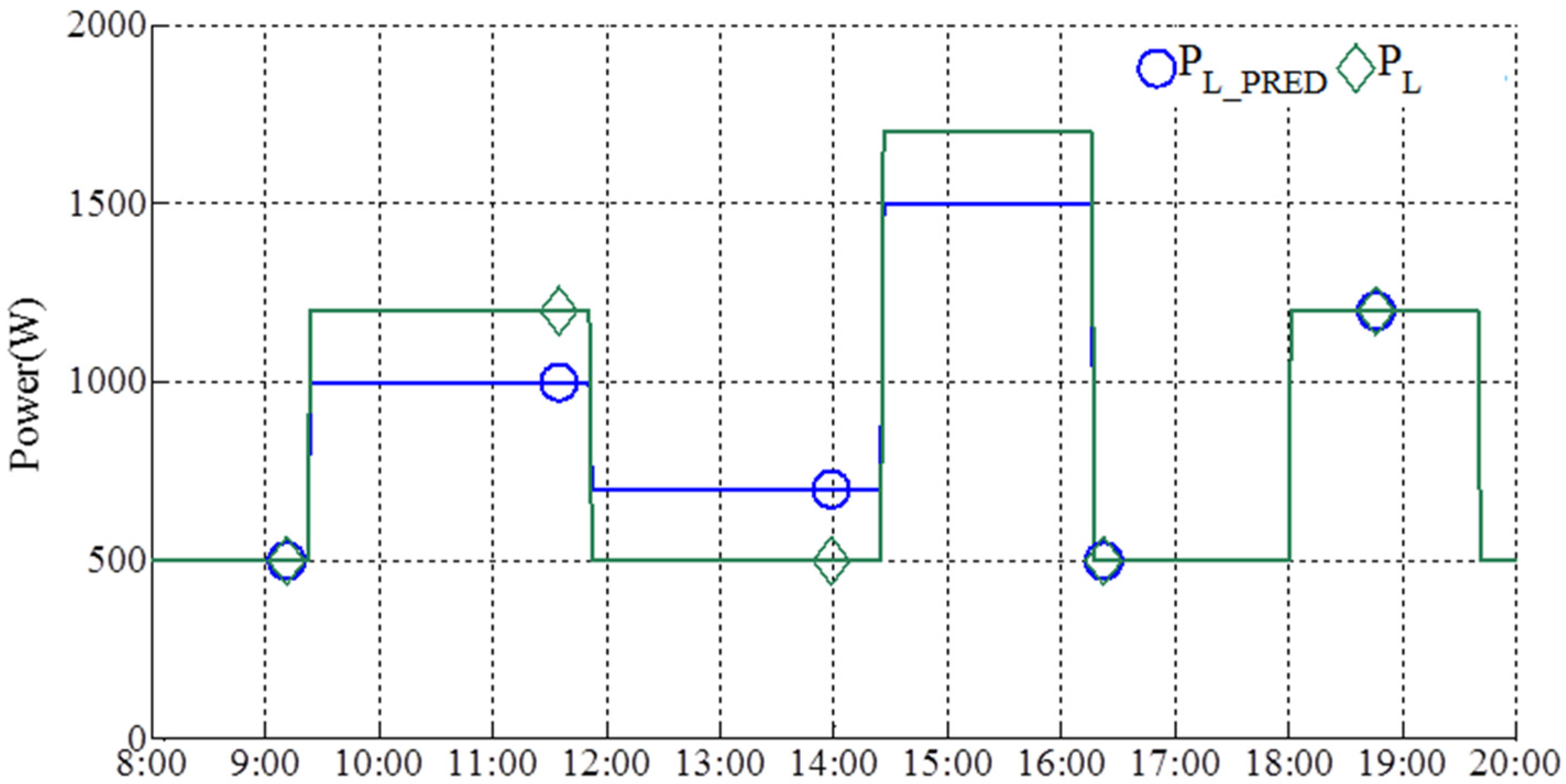
Regarding the actual load power and its prediction, for all experimental tests, they are considered arbitrary. Load power represents DC building consumption as shown in Figure 6.

Figure 6. Load power prediction P_{L_PRED} and load power demand P_L for experimental tests.

Figure 6. Load power prediction P_{L_PRED} and load power demand P_L for experimental tests.

Three experimental tests are operated. Depending on meteorological day profile, the case studies retained are: high solar irradiance almost without fluctuations (Test 1), high solar irradiance with strong fluctuations (Test 2), and mixed high irradiance with strong fluctuations and low irradiance without fluctuations (Test 3).

4.1. Test 1

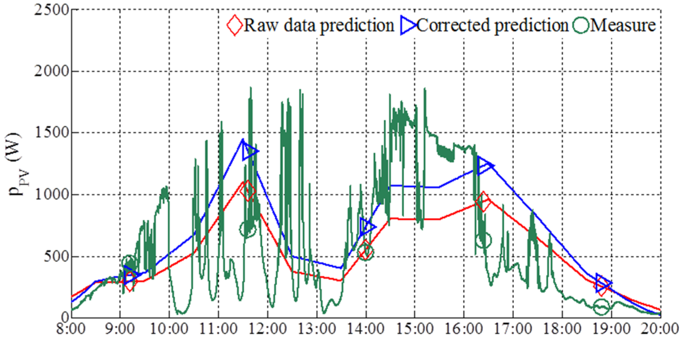
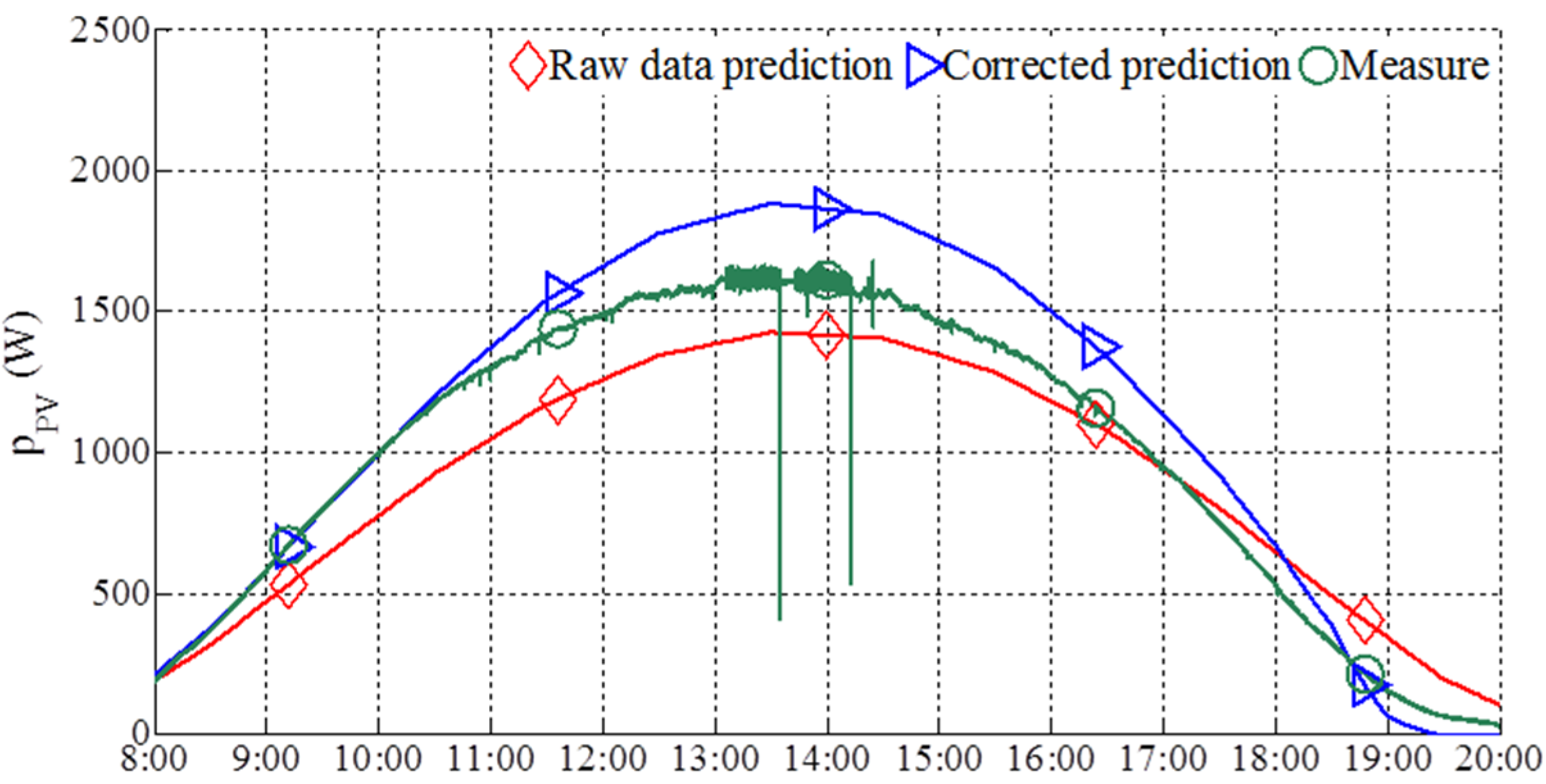
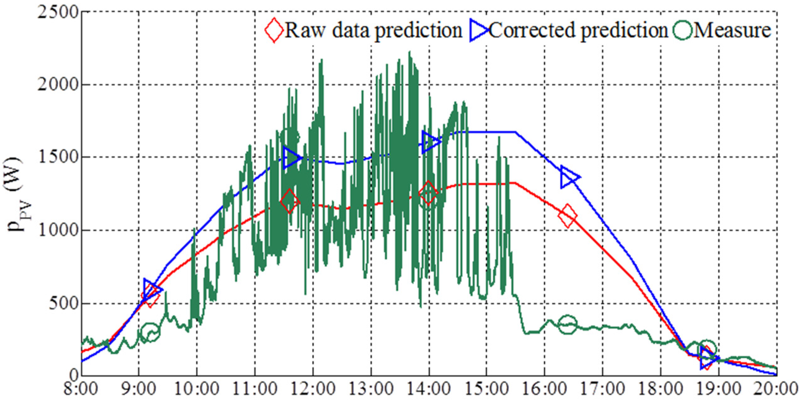
Test 1 is performed for operation on the 4 September 2013 in Compiegne, France [30]. A few minutes ahead the test, based on solar irradiation hourly forecast data and PV source model [29], the PV sources power prediction is calculated and also corrected to correspond to the PV panels tilt. The PV sources power uncertainty is shown in Figure 7.

Figure 7. PV sources power prediction for experiment and PV sources power measure for Test 1.

Figure 7. PV sources power prediction for experiment and PV sources power measure for Test 1.

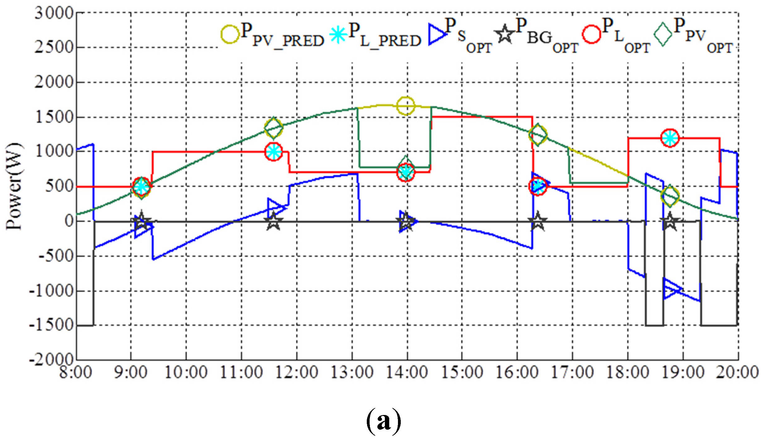
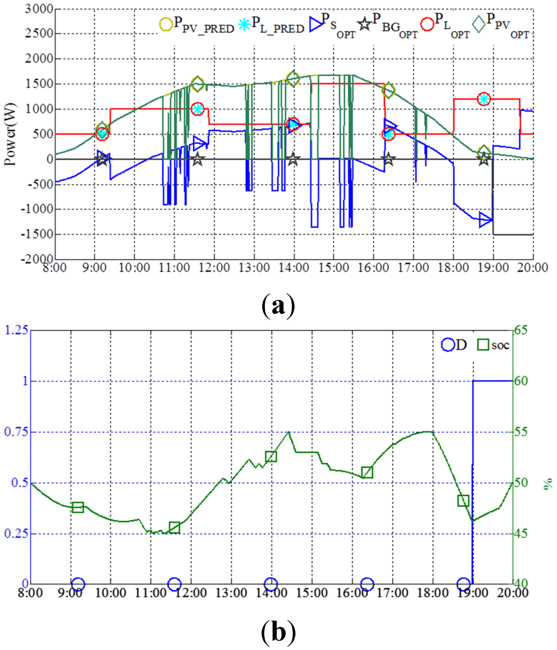
Based on these predictions, the microgrid optimizes the power flow by CPLEX as shown in Figure 8a. Concerning the power flow curves, note that for storage, negative power means supplying the load, while positive means receiving power. For graphical clarity biofuel generator power is represented by negative values. The proposed optimization shows that the storage is used for power balancing and the biofuel generator is started by duty cycles in order to keep continuous supply for the load and ensure that at the end of the operation the storage capacity is above a preferred level SOC_F.

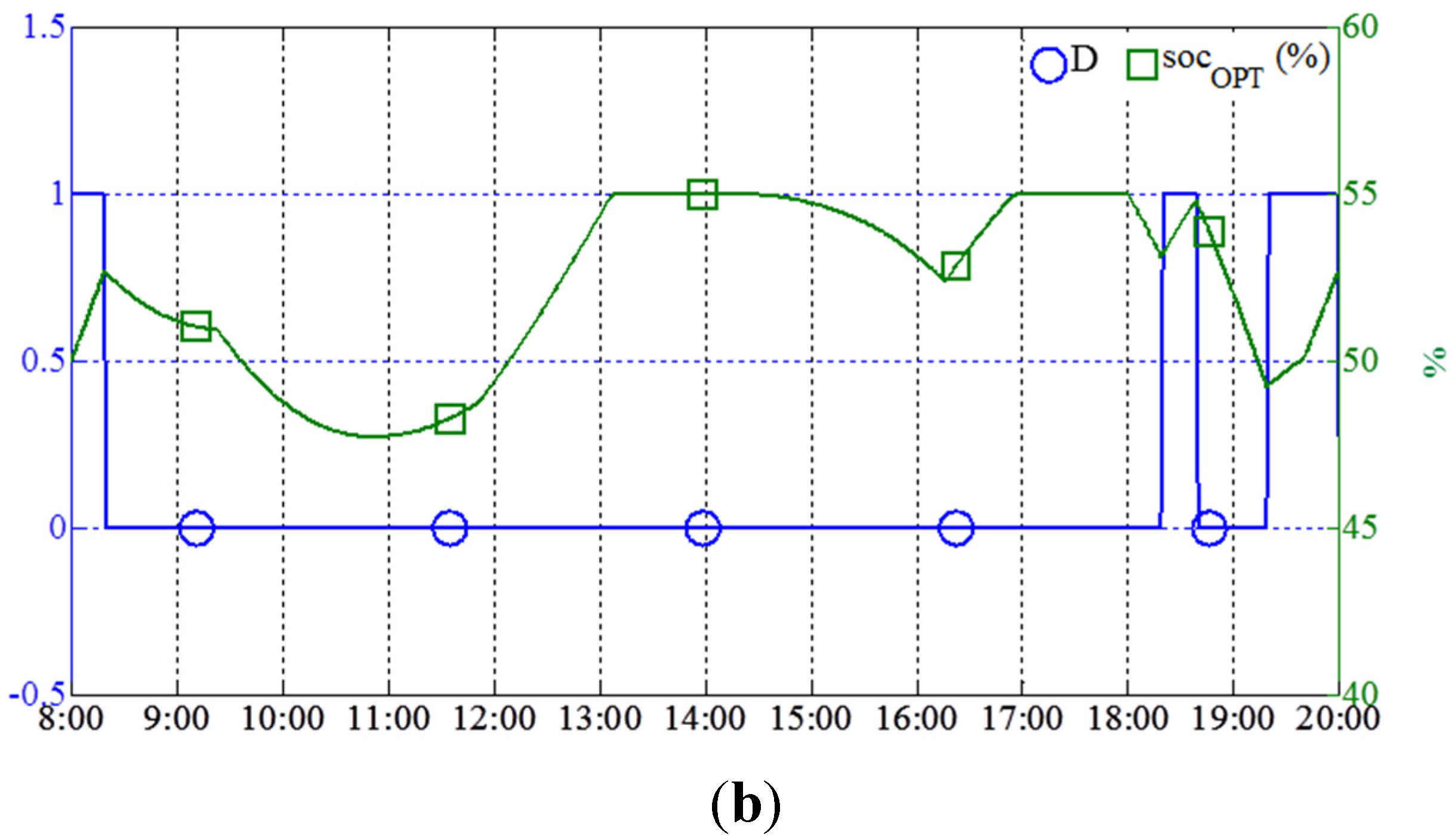
Figure 8. (a) Predicted and optimized power flow for Test 1; (b) D and soc evolution given by optimization for Test 1.

Figure 8. (a) Predicted and optimized power flow for Test 1; (b) D and soc evolution given by optimization for Test 1.

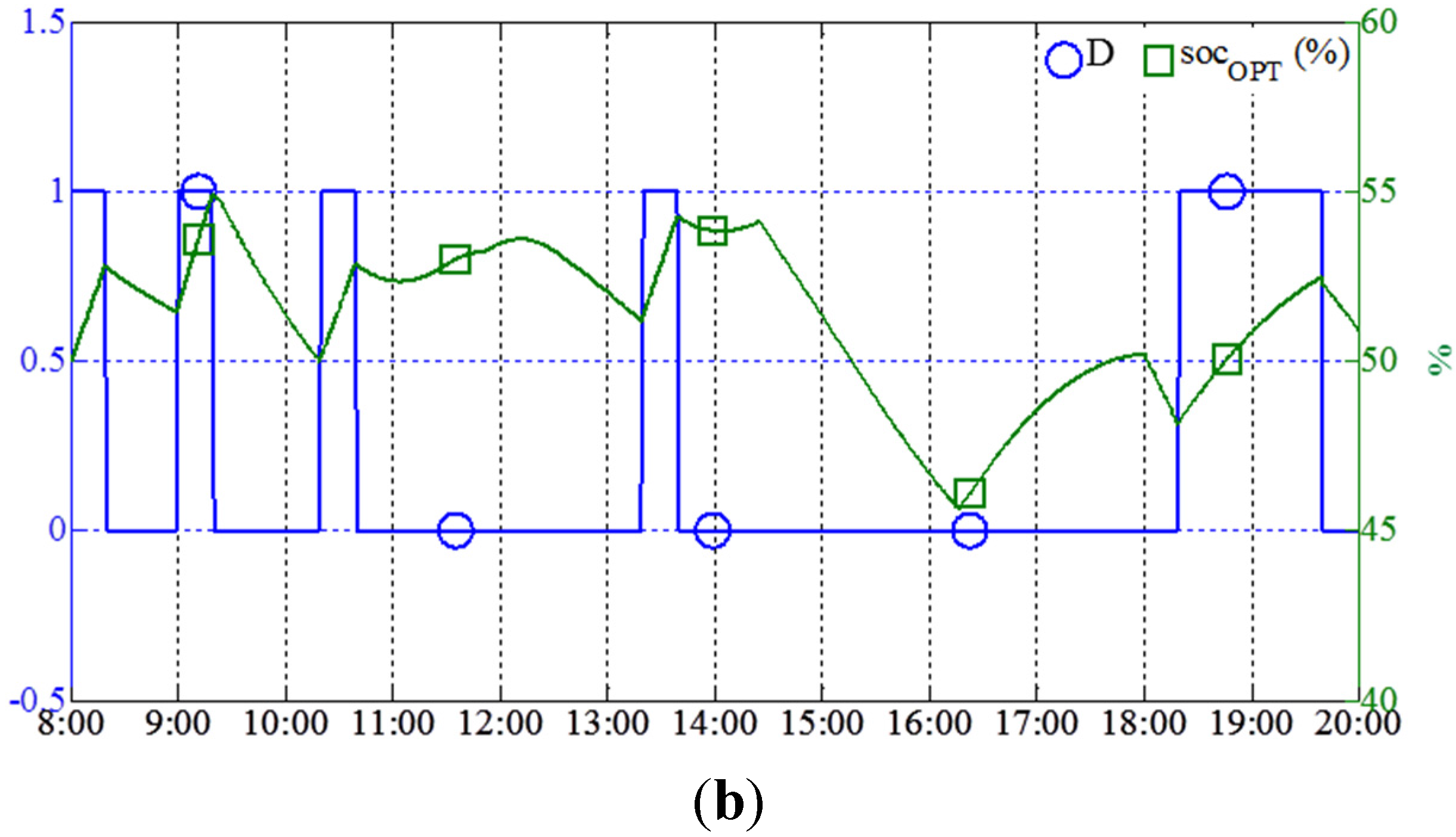
When the storage reaches SOC_MAX, the only way to keep power balancing is to limit PV sources power production; this is why there is PV sources power limiting in the period of 13:10–14:20. Optimum $D$ time series sequence, calculated as the on-off signal for the biofuel generator, and the estimated $soc$ evolution given by the optimization are shown in Figure 8b.

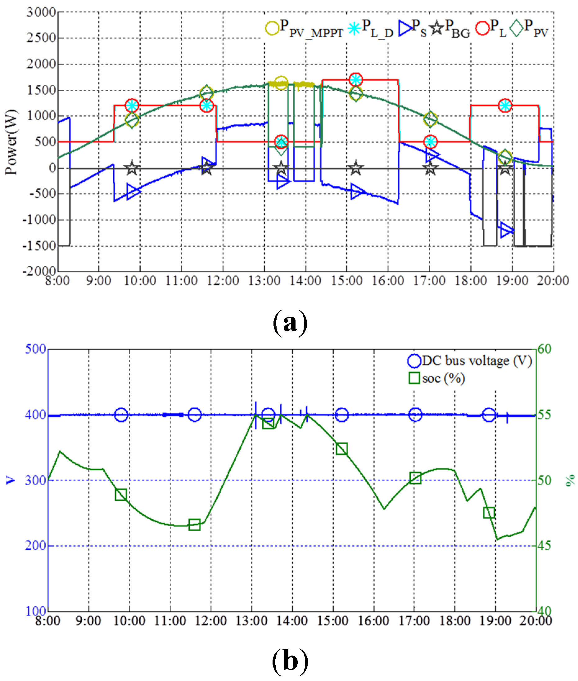
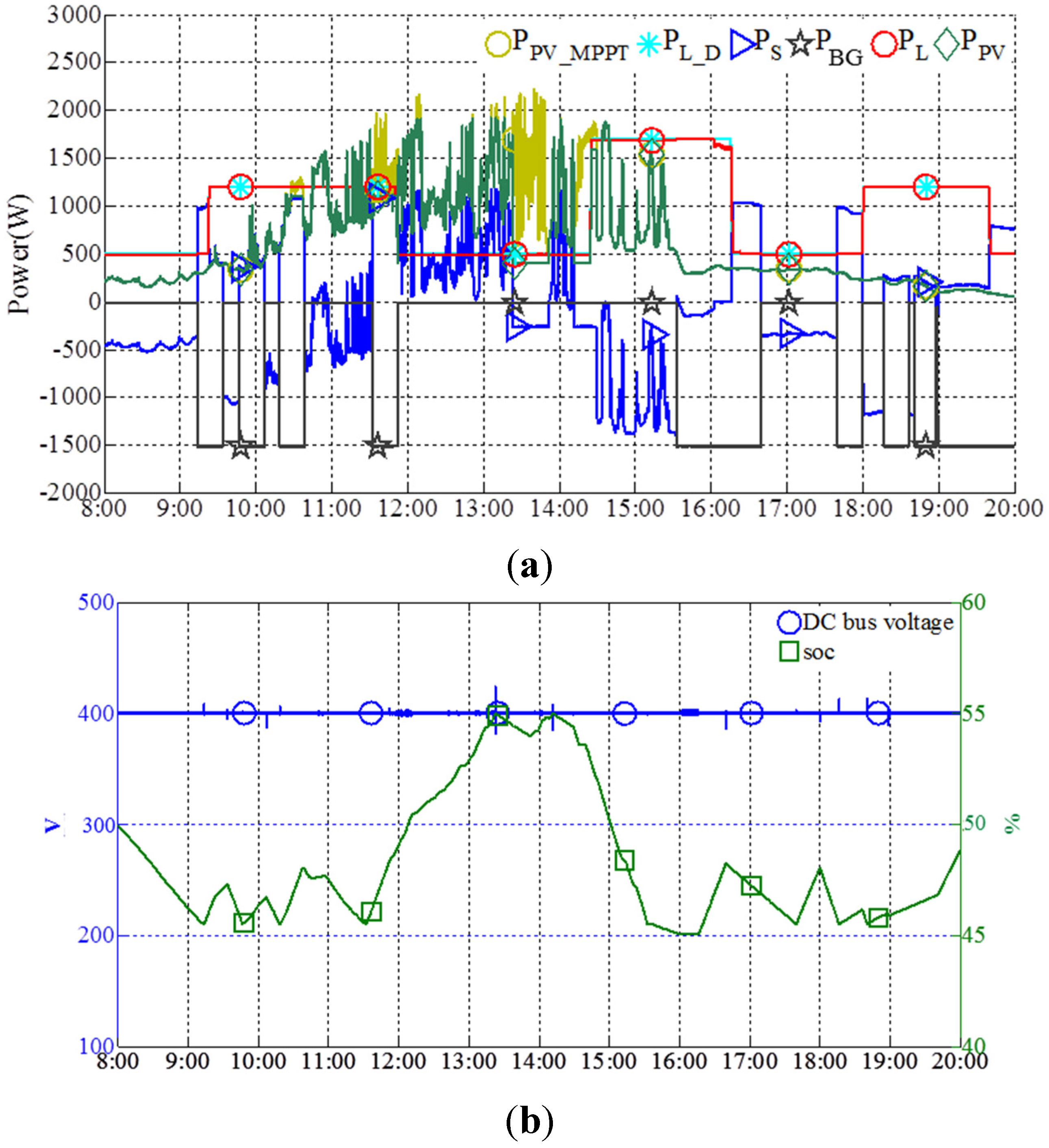
The operation is performed based on $D$ and the power balancing control algorithm. The experimental real-time power flow is shown in Figure 9a. The experimental $soc$ and DC bus voltage evolution are shown in Figure 9b.

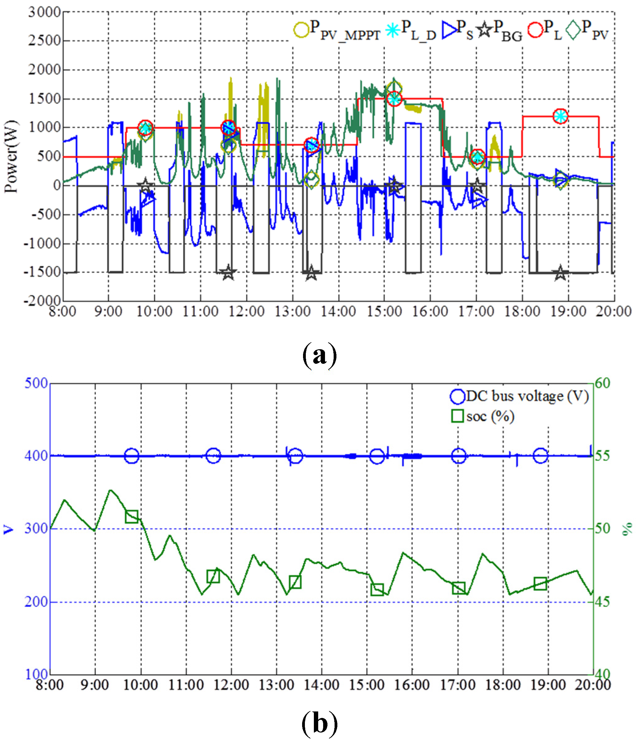
Figure 9. (a) Experimental real-time power flow for Test 1; (b) Experimental DC bus voltage and soc evolution for Test 1.

Figure 9. (a) Experimental real-time power flow for Test 1; (b) Experimental DC bus voltage and soc evolution for Test 1.

In this test, biofuel generator is started by duty cycle as commanded by $D$ for 8:00–8:20, 18:20–18:40, 19:20–20:00. No load shedding is performed. During 8:00–13:05, the power is balanced following $D$. Despite uncertainties in both load and PV sources power prediction, the storage is fully charged around 13:05, as expected by optimization. During 13:05–14:20, there is no other possibility that can absorb PV sources production, and it is hard to calculate the PV sources power limiting reference to produce the accurate power needed by the load. As a solution, the control strategy slightly over limits the PV production, inducing storage discharging with low power. After the $soc$ is reduced by certain amount, the PV sources are recovered to produce MPPT power again until the SOC_MAX is reached again. That is why the PV sources power oscillation between MPPT mode and power limiting mode can be observed.

During 14:20–20:00 two differences relative to the optimization can be noted: firstly, the PV sources power limiting during 16:55–18:00 is not carried out in actual power flow since actual higher load power than PV production caused $soc<SO{C}_{MAX}$; secondly, biofuel generator is started during 19:00–19:20, which is controlled by the power balancing control algorithm that starts biofuel generator when $soc$ approaches SOC_MIN.

As presented in Figure 9b, due to uncertainties, the final $soc$ value is less than 50%. The power is well balanced during the operation, as shown in Figure 9b by the steady DC bus voltage. The DC bus voltage fluctuates about 5% at the instants of limiting PV power and starting biofuel generator control, which is related to corresponding control dynamics and is acceptable. The DC bus voltage pulse is generally coming from two sides: on the one hand, the voltages and currents are filtered and the powers are calculated by the filtered signals; on the other hand, power references to stabilize the DC bus voltage are compensated by the filtered power, which is filtered as well and so it has a delay in time. This problem, whose development is not considered here, could be solved by using less filtered signal or improving the performance of correctors in order to cancel the compensation.

Table 2 shows the total energy cost C_total based on energy tariff (€/kWh) given in Table 1 (c_BG, c_S, c_PVS, c_LS) and taking onto account the operating time period of 12 h taken into account, i.e., from 8:00 to 20:00.

Table 2. Energy Cost Comparison.

Case Operation	Energy Cost Ctotal (€)
Estimated optimum energy cost following power predictions	3.629
Actual energy cost (experiment)	3.658
Optimum energy cost for real conditions calculated after operation	3.380

Table 2. Energy Cost Comparison.

Case Operation	Energy Cost Ctotal (€)
Estimated optimum energy cost following power predictions	3.629
Actual energy cost (experiment)	3.658
Optimum energy cost for real conditions calculated after operation	3.380

The total energy cost C_total is calculated for three cases: estimated optimum energy cost following power predictions, the experimental cost, which is the actual energy cost, and the optimum energy cost for real conditions calculated after operation. Thus, the actual energy cost is higher than the estimated cost by optimization before the operation; it is due to uncertainties. Aiming at a fair comparison, the total energy cost is calculated again at the end of the test based on real test conditions and using the optimization problem formulation. In this last case, the obtained cost is the total optimum energy cost that would have been possible to achieve following the real solar irradiation and the real load power. The difference between the actual total energy cost and the total optimum energy cost is about 8% for this experimental test. Given this small difference, the optimization problem formulation could be considered as demonstrated.

4.2. Test 2

Test 2 is performed for operation on 27 August 2013. PV sources power prediction uncertainty is shown in Figure 10. It can be noted that the measure is less than the corrected prediction and for the periods of 8:00–10:00 and 15:30–20:00 the weather is heavily cloudy which is not predicted.

Figure 10. PV sources power prediction and actual PV sources power measure for Test 2.

Figure 10. PV sources power prediction and actual PV sources power measure for Test 2.

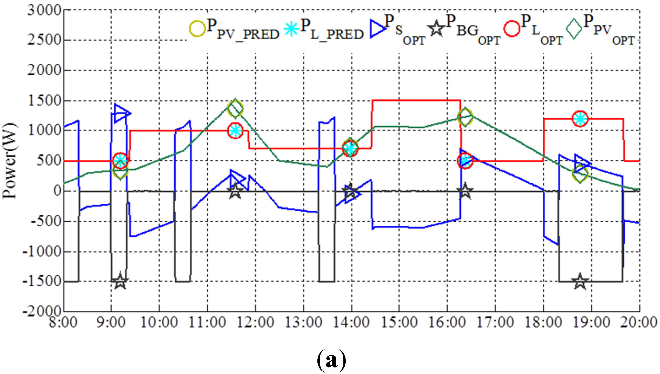
The optimized power flow by CPLEX is shown in Figure 11a. As aforementioned, when the storage reaches SOC_MAX, the only way for keeping power balancing is to limit PV production; therefore, PV sources limited power control must be performed. In this case, the limited PV production is distributed randomly during 10:45–17:20. Based on optimum power flow evolution, optimum D sequence is calculated for the experimental operation, which represents the on-off state for the biofuel generator, as shown in Figure 11b.

Figure 11. (a) Predicted and optimized power flow for Test 2; (b) D and soc evolution given by optimization for Test 2.

Figure 11. (a) Predicted and optimized power flow for Test 2; (b) D and soc evolution given by optimization for Test 2.

Based on the power balancing algorithm, which implies the use of the control parameter $D$, the operation is performed and the obtained power flow is shown in Figure 12a. Experimental $soc$ and DC bus voltage evolution are shown in Figure 12b.

Figure 12. (a) Experimental real-time power flow for Test 2; (b) Experimental DC bus voltage and soc evolution for Test 2.

Figure 12. (a) Experimental real-time power flow for Test 2; (b) Experimental DC bus voltage and soc evolution for Test 2.

During this day operation, storage is used for regulating the power balance. The biofuel generator is started with interface value $D=1$ for 19:00–20:00 as commanded by optimization or when the $soc$ approaches SOC_MIN, i.e., 9:10–9:30, 9:45–10:05, 10:15–10:35, 11:30–11:50, 15:40–16:40, 17:40–18:00, 18:15–18:35, 18:37–18:57, which are controlled by power balancing strategy.

Storage power is limited to avoid high power charging by high PV sources plus biofuel generator that can shorten the storage lifetime. Therefore, in the case when redundant power exceeds storage power limit, the PV production is limited to protect storage, i.e., 10:20–10:35 and 11:30–11:50. When storage reaches SOC_MAX, PV sources power limiting is performed during 13:20–13:50. To avoid oscillation, the PV sources limited power control is recovered with hysteresis as aforementioned in Test 1.

Load shedding is performed as another control degree of freedom in the case when storage is empty and biofuel generator plus PV sources power cannot supply the load demand, i.e., 16:00–16:15. In this case, the prediction uncertainty is significant, so more biofuel generator production is performed. Nevertheless, the power balancing is able to be maintained as indicated by steady DC bus voltage in Figure 12b. Due to prediction uncertainties, it can be seen that biofuel generator is started more than expected in order to keep continuous load supply.

Table 3 compares the energy cost among optimization, experiment, and optimum for real conditions. The experimental cost is much greater than the estimated cost by optimization.

Table 3. Energy Cost Comparison for Test 2.

Case Operation	Energy Cost Ctotal (€)
Estimated optimum energy cost following power predictions	3.259
Actual energy cost (experiment)	7.807
Optimum energy cost for real conditions calculated after operation	7.596

Table 3. Energy Cost Comparison for Test 2.

Case Operation	Energy Cost Ctotal (€)
Estimated optimum energy cost following power predictions	3.259
Actual energy cost (experiment)	7.807
Optimum energy cost for real conditions calculated after operation	7.596

The difference is obvious, since more biofuel generator production is involved to ensure power balance, when in real conditions the PV production is much less than expected by prediction. However, the experimental cost is close to optimum energy cost for real conditions calculated after the experiment.

4.3. Test 3

Test 3 is performed on 6 September 2013. PV sources power prediction uncertainty is shown in Figure 13. The prediction can correspond the two peak periods of production.

Figure 13. PV sources power prediction and actual PV sources power measure for Test 3.

Figure 13. PV sources power prediction and actual PV sources power measure for Test 3.

The optimized power flow by CPLEX is shown in Figure 14a. As the solar irradiance is relatively low, no PV sources power limiting is performed. Based on optimum power flow evolution, optimum $D$ sequence is given in Figure 14b.

Figure 14. (a) Predicted and optimized power flow for Test 3; (b) D and soc evolution given by optimization for Test 3.

Figure 14. (a) Predicted and optimized power flow for Test 3; (b) D and soc evolution given by optimization for Test 3.

The obtained experimental power flow is shown in Figure 15a. Experimental $soc$ and DC bus voltage evolution are shown in Figure 15b.

Figure 15. (a) Experimental real-time power flow for Test 3; (b) Experimental DC bus voltage and soc evolution for Test 3.

Figure 15. (a) Experimental real-time power flow for Test 3; (b) Experimental DC bus voltage and soc evolution for Test 3.

Identical to Test 2, storage power is limited to avoid high power charging by high PV sources power plus biofuel generator production that can shorten the storage lifetime. Therefore, in case of storage injection power tending to exceed storage power limit P_{S_MAX}, the PV production is limited to protect storage (around 9:10, 10:30, 11:30, 12:30, 15:40 and 17:20). It can be seen that the biofuel generator is started more than expected in order to maintain a continuous load supply.

The uncertainties make the actual instantaneous power evolution different as predicated. Nevertheless, the power balancing is able to be maintained and load can be supplied without load shedding. The power balancing is indicated by steady DC bus voltage in Figure 15b.

The energy cost calculations are given in Table 4 which validates again that in real conditions the experimental cost is close to optimum energy cost for real conditions calculated after operation.

Table 4. Energy Cost Comparison for Test 2.

Case Operation	Energy Cost Ctotal (€)
Estimated optimum energy cost following power predictions	4.366
Actual energy cost (experiment)	6.689
Optimum energy cost for real conditions calculated after operation	6.017

Table 4. Energy Cost Comparison for Test 2.

Case Operation	Energy Cost Ctotal (€)
Estimated optimum energy cost following power predictions	4.366
Actual energy cost (experiment)	6.689
Optimum energy cost for real conditions calculated after operation	6.017

5. Analysis and Discussion

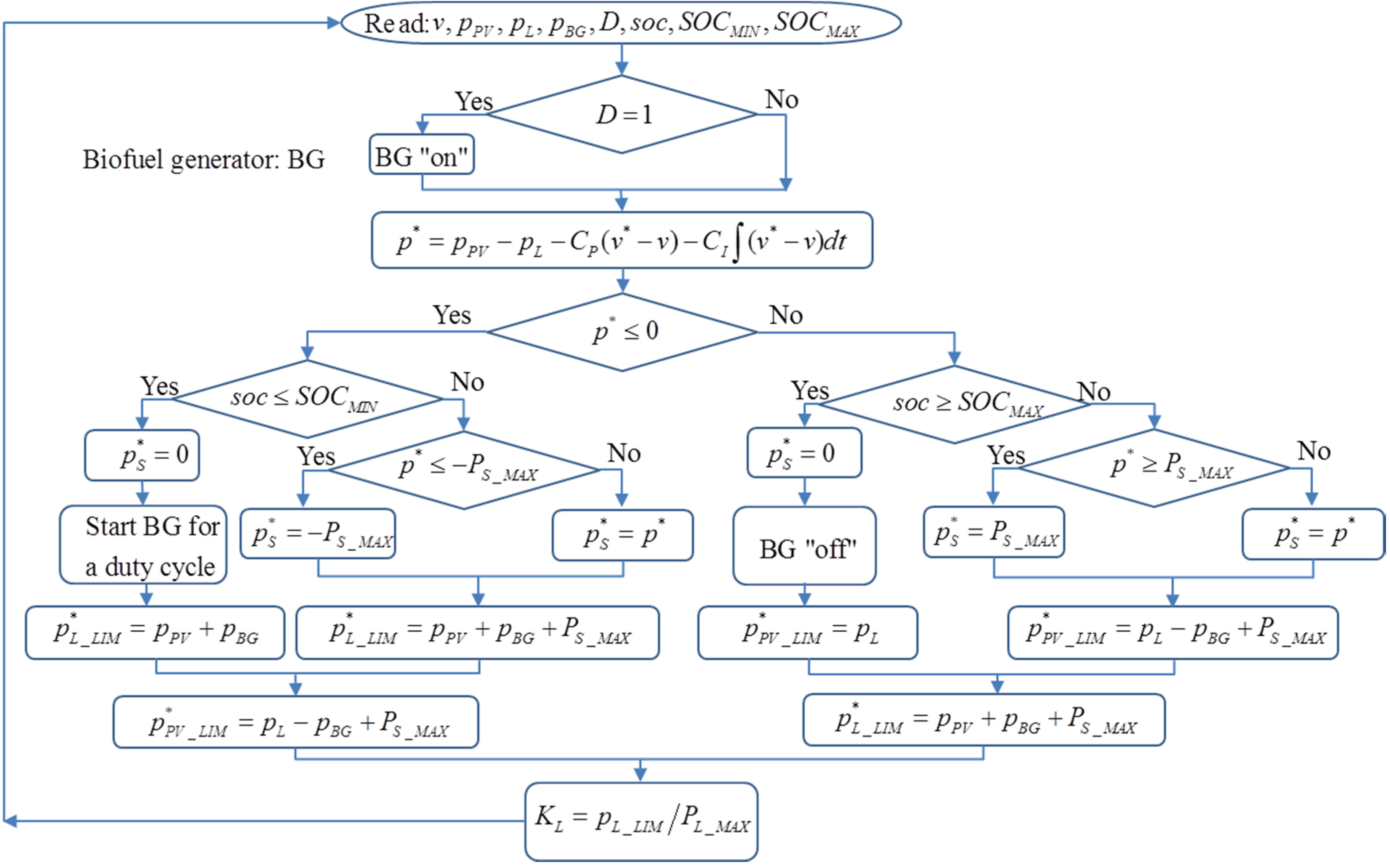
The optimization objective is to minimize biofuel consumption and keep certain storage capacity at the end of the operation. The experimental tests validate the proposed control strategy which can work under different weather conditions for providing robust power balancing while taking into account optimization results. As $D$ is defined as switch for biofuel generator operation, its values are given for each optimization case study. Regarding the experimental tests, the $D$ values can be seen following the evolution of biofuel generator power curve (p_BG in black): when biofuel generator starts and outputs the rated power $D=1$; when biofuel generator has no specific order $D=0$. It can be noted that for experimental test, the real sequence $D$ is not always identical to that the optimization gives. This shows that the proposed control algorithm is robust and able to maintain the power balancing with self-correcting ability and not only to follow the predicted optimization operation.

Table 5 summarizes the comparison of the cost of energies between the operated three tests.

Table 5. Energy cost comparison between the operated three tests.

Test	Case Operation	Total Energy Cost (€)	Load Shedding Cost (€)	PV Power Limiting Cost (€)	Biofuel Generator Production Cost (€)
	Optimization	3.629	0	1.463	2.166
1.	Experimentation	3.658	0	1.121	2.423
	Optimization for real conditions	3.380	0	1.180	2.2
	Optimization	3.259	0	1.575	1.684
2.	Experimentation	7.807	0.211	0.835	6.761
	Optimization for real conditions	7.596	0	1.030	6.566
	Optimization	4.366	0	0	4.366
3.	Experimentation	6.689	0	0.175	6.514
	Optimization for real conditions	6.017	0	0.001	6.016

Table 5. Energy cost comparison between the operated three tests.

Test	Case Operation	Total Energy Cost (€)	Load Shedding Cost (€)	PV Power Limiting Cost (€)	Biofuel Generator Production Cost (€)
	Optimization	3.629	0	1.463	2.166
1.	Experimentation	3.658	0	1.121	2.423
	Optimization for real conditions	3.380	0	1.180	2.2
	Optimization	3.259	0	1.575	1.684
2.	Experimentation	7.807	0.211	0.835	6.761
	Optimization for real conditions	7.596	0	1.030	6.566
	Optimization	4.366	0	0	4.366
3.	Experimentation	6.689	0	0.175	6.514
	Optimization for real conditions	6.017	0	0.001	6.016

Experimental results show that the proposed microgrid structure is able to implement optimization in real power control and ensures self-correcting capability. The power flow can be controlled to approach optimum cost when the prediction error is within certain limits. Even if the prediction is quite imprecise, the power balancing can be maintained with respect of rigid constraints.

It is obvious that the optimization effectiveness depends on prediction precision. In the first test, despite of the biofuel generator duty cycles assigned by optimization, biofuel generator is started for one more duty cycle by operation control algorithm. More biofuel generator duty cycle is started for the second test, but the final $soc$ is close to 50%. In the third test, the final $soc$ is far from 50%. Load shedding occurs only in Test 2, though it was not expected in the optimization. This is due to a relatively large gap between the solar irradiance prediction and reality, on the one hand, and the imposed limits to storage, on the other hand. Regarding the PV sources shedding, there are differences between optimization and experimentation in all three tests; however, these facts do not affect the total energy costs.

Generally, besides the prediction precision, other factors that affect the effectiveness exist such as converter efficiency and control security margin. As the general prediction data is provided for a large area about 20 km², for a single location, the prediction precision may not be satisfactory, especially for cloudy weather conditions. Improvement can be done by adding local forecasting techniques such as sky camera and local weather measurement and forecasting station. On the other hand, for these tests, the storage is used for only 10% of its capacity that corresponds to the energy of 1.25 kWh; however, this condition is imposed just to show more control event during a day test. Certainly, a larger storage capacity could be more resistant to the prediction errors.

The experimental costs, which are the actual energy costs, are different from the estimated cost by anterior optimization; this is due to forecast uncertainties. In posterior optimization for real conditions case, the obtained costs are the ideal optimum energy costs that could be reached following the real solar irradiation and the real load power. Indeed, this calculation is performed by completely eliminating uncertainties. Therefore, the total energy cost, as result of this operation, can be considered the indicator of optimum operating. This indicator would be helpful to analyze the system behavior, but its calculation is not possible until the end of the operation. The results presented in Table 5 highlight the role of uncertainties in microgrid control to obtain the minimum energy cost. The gap between the indicator and the actual outcome depends heavily on gap between the meteorological forecast data and actual measurements.

Even with uncertainties, the experimental cost can be controlled close to optimization for real conditions cost, which is the ideal experimental cost. Thus, it can be considered that these results validated the effectiveness of the proposed optimization and power management control. The power balancing can be maintained and rigid constraints such as storage power limit, storage capacity limit are fully respected.

6. Conclusions

The microgrids systems will become more and more complex and selective according to needed applications. For tertiary buildings equipped with renewable energies, which form an isolated DC microgrid, the overall performance of a building-integrated microgrid is improved by the use of DC electric distribution bus instead of AC distribution bus. This paper shows the interest in the improvement of the overall system efficiency for the local production, local consumption, and usages.

Regarding the islanded DC microgrid operation, optimal scheduling and real-time power management are presented in this paper. Aiming to minimize the total energy cost and based on forecasting data, a cost function is formulated and solved. Thus, based on this prediction-based optimization, for real-time power balancing, the experimental results validate the feasibility of the proposed control of islanded DC microgrid. The minimization of the total energy cost is possible and its implementation could be interesting and does not require high cost. However, the optimization efficiency is based on the power predictions precision. Prediction uncertainties do not influence power balancing but the optimal energy cost is affected. Future work may focus on the impact reducing of uncertainties. One approach could be to re-perform the optimization calculation during the operation with latest forecasting data and real-time system status without interrupting power balancing. In further work real-time optimization will be re-performed with hourly updated weather forecast.