The Impacts of Environmental Tax in China: A Dynamic Recursive Multi-Sector CGE Model

Abstract

In recent years, the accumulated environmental problems resulting from excessive usage of fossil fuels have gradually loomed. Thus, an environmental tax, as an important policy tool, has been put on the agenda in China. In this paper, a dynamic recursive multi-sector Computable General Equilibrium (CGE) model is applied to explore the impacts of the environmental tax on China’s economy. To comprehensively analyze the impacts, we introduce four kinds of typical contaminants and set two kinds of scenarios: different tax rates and different tax refunds. The results show that the environmental tax is conducive to environmental improvement, but the economic variables are adversely affected, for example, the loss of GDP at the low level tax rate is 0.46%. In order to offset the negative impacts, we presume the government refunds the tax. The results show that this can indeed relieve the negative effects. When the government refunds the production tax and corporate income tax, 0.49% and 0.34% of GDP is relieved by respectively. This paper provides a comprehensive analysis of the implementation of the environmental tax in China and lays a solid foundation for the introduction of the environmental tax.

1. Introduction

Although the Chinese people are proud of the rapid development of the economy, the fact of China’s heavy reliance on fossil fuels causes severe environmental problems and health problems for dwellers. Carbon dioxide, sulfur dioxide, nitrogen oxide and carbonic oxide are the main atmospheric pollutants that currently affect Chinese air quality, and can also have important effects on the global climate and human health [1]. All these atmospheric pollutants mainly come from the usage of fossil energy. In 2010, there were 8.29 billion tons of carbon dioxide, 21.85 million tons of sulfur dioxide, and 18.52 million tons of nitrogen oxide emissions.

In recent years, the environmental deterioration tendency has not been effectively controlled yet. Global climate change has become a hot topic throughout the world. Several reports issued by the IPCC (Intergovernmental Panel on Climate Change) have pointed out that climate change is closely related to human activities [2,3,4,5]. There are growing calls around the world to reduce pollutant emissions. Countries have committed to participate in international efforts to combat climate change. Hence, mounting pressure from the international community requires that a series of emission reduction targets and emission mitigation policies should be implemented by the Chinese government. In the context of pursuing climate policy targets for 2020 (the emissions per unit of GDP are required to be reduced by 40% to 45%), a number of economists exceptionally value market-based climate management tools, to strive to minimize the economic costs in realizing the given emission reduction goals. Meanwhile, they have applied various alternative methods to discuss the environmental policy, such as system dynamics model [6], macro-econometric model [7] and computable general equilibrium model [8]. Of these approaches, the Computable General Equilibrium (CGE) model stands out due to its solid theoretical basis and comprehensive model framework.

The first environmental CGE model was set up by Dufournaud, who introduced pollutant emissions and control behavior into the CGE model, then the environmental CGE model was thus built [9]. Since then, a large number of scholars began to establish environmental CGE models. The use of CGE models started relatively late in China, especially environmental CGEs, but in recent years, it has emerged rapidly and there is an increasing amount of research focused on China.

Researches on the level of duties on pollutants emissions have been done in the past few years, mainly to determine the right tax rate that can reduce pollutants emissions and help minimize the adverse impacts on economic operations [10,11,12]. Unfortunately different literatures suggested different tax rates, and the optimal tax rate still remains a controversial topic. Recently, The Finance Fiscal Science Research Institute issued a scientific study and put forward that coal resources tax should continue to apply in 2015 and a low-level environmental tax should be introduced in China around the year 2019 [13]. Given the difficulty in determining the right tax rate, many scholars have set emission reduction as the target and value the adverse impacts on economic operations. There is extensive literature on emission reduction targets, and the specific duty imposed by the environmental tax is determined by emission reduction in all sectors, and each sector has different tax rates according to the different emissions [14,15,16,17,18].

Gradually, many scholars have noticed that environmental policy can inevitably induce negative impacts on the whole of society. Only valuing the tax rate or emission reduction is no longer enough, and they began to consider the concept of “tax neutrality”. The most common way to use the environmental tax is to recycle the tax revenue, which, to some extent, can avoid some negative impacts and also can relieve the distortion of the tax [19,20,21,22,23,24,25].

We can notice that some of the studies we mentioned above used static models to analyze the impacts of a carbon tax. A static model can only simulate the impacts on the base year and cannot measure the long-term effects. Undoubtedly the variation between short term and long term can reveal the process of market adjustment which is important to policy makers. What’s more, most researchers only studied the different tax rates or different tax refund methods, which cannot comprehensively analyze the impacts of an environmental tax. Additionally, the analysis on the industry level is not well addressed in the previous studies.

Therefore, this paper contributes to the literatures in two ways: first, we have disaggregated the industries and energy sectors, which allows us to explore the impact of the environmental tax on both the macroeconomic level and industry level; second, we assessed the macroeconomic impacts of an environmental tax and the effects of refunds as a way of offsetting negative impacts in China. To achieve the objectives, we performed a scenario analysis combining different tax rates and different tax refunds.

The rest of the paper is organized as follows: Section 2 discusses the model structure used in this study; Section 3 provides two different kinds of scenarios; Section 4 shows the simulation results; Section 5 discusses the implications of simulations; Section 6 contains conclusions and policy implications.

2. Method and Methodology

A dynamic recursive multi-sector computable general equilibrium model is developed to simulate the impacts of the environmental tax on China’s economic market. In this CGE model, the economic activities are categorized into several modules, that is, production block, trade block, income and expenditure as well as model closures and market clearing. Moreover, the environment block is introduced into the model to embed the four kinds of pollutant emissions: CO₂, SO₂, NO_x, and CO. The static CGE structure of this paper is shown in Figure 1. In addition, the dynamic mechanism is embedded in this model; the dynamic algorithm is also illustrated in Figure 1. As for the details of each subdivision, they are shown in the following pages.

Common forms of production functions are the Leontief function, linear function, Cobb-Douglas function and constant elasticity of substitution production function. The constant elasticity of substitution production function, or simply “CES” for short, is the most commonly used nonlinear function in the CGE model, or more broadly, not only in the production module, but also widely used in the utility function and distribution function of production-possibility frontier. e.g., constant elasticity of transformation function (CET), at least formally, is a transformation of the CES function.

The production side of the CGE is modeled using a series of nested CES production functions so as to allow for substitutability between usages of commodities in the production:

$$\min \sum _{i=1}^n{p}_i\cdot x_i$$

(1)

$$s.t.f(x_1,x_2\cdot \cdot \cdot x_n)=\alpha {[{\delta }_1{x}_1^{\rho }+{\delta }_2{x}_2^{\rho }+\cdot \cdot \cdot +{\delta }_n{x}_n^{\rho }]}^{\raisebox{1ex}{$1$}\!\left/ \!\raisebox{-1ex}{$\rho $}\right.}$$

(2)

where $\alpha$ is the share parameter of CES, ${\delta }_n$ is the transfer parameter of CES, and $\rho =\raisebox{1ex}{$1$}\!\left/ \!\raisebox{-1ex}{$1-\sigma $}\right.$, $\sigma$ is the substitution elasticity between x_i, p_i is the price of x_i.

Figure 1. The static Computable General Equilibrium (CGE) and the structure of CGE model in this paper.

Figure 1. The static Computable General Equilibrium (CGE) and the structure of CGE model in this paper.

2.1. Production Block

The top layer (total output) of the nested structure comprises the composite primary inputs of the intermediate inputs, labor, capital, and energy (Electricity, Coal, Crude oil, Gas, Petroleum). Beginning in the top-most nest of Figure 2, we presume the Non-energy intermediates input and the value-added comprise the total output at substitution elasticity ${\sigma }_a^a$. Then, the second layer determines the producers’ demand for the labor inputs and for the composite of capital and energy at substitution elasticity ${\sigma }_a^{va}$ that is disaggregated into capital and energy in the third layer at substitution elasticity ${\sigma }_a^{ke}$. In the next three layers, the energy input is gradually disaggregated into electricity, coal, crude oil, gas, and petroleum. We presume the producers can substitute between crude oil, gas, and petroleum, so these energies are combined at substitution elasticity ${\sigma }_a^{nc}$. Then the CES aggregate of Oil-Gas energy can then be combined with Coal energy in the next-higher nest at substitution elasticity ${\sigma }_a^c$. Ultimately, the CES aggregate of fossil energy can then be combined with electric power in the next-higher nest at substitution elasticity ${\sigma }_a^e$. Given fossil fuels are the primary source of electricity, the substitution elasticity between electricity and fossil fuels should be smaller than those between fossil fuels [26]. Furthermore, as the material basis for the production, the substitution elasticity of the energies is smaller than other commodities. It is noteworthy that the substitutability of electricity is relatively weaker than other energies, so the elasticity of electricity is relatively smaller than other energies. The details of the substitution elasticity for the functions are discussed in Appendix A.

Figure 2. An overview of the production structure.

Figure 2. An overview of the production structure.

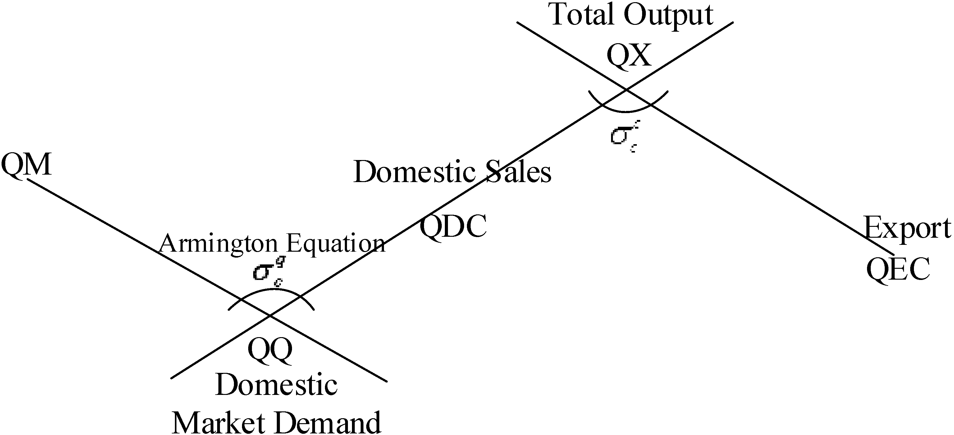
2.2. Trade Block

Part of the domestic total outputs are supplied for export, and the rest are used for supplying the domestic market. The problem of two-way trade always appears when considering the trading data, which means a given type of commodities are both exported and imported simultaneously. An effective way to solve this problem is assuming commodities belong to different countries have imperfect substitutability.

According to Armington, the trade block is incorporated into the CGE model by treating imported and domestic commodities as differentiated products, and this behavior can be depicted by CES equation. We assume that commodities in domestic market are CES aggregates of imported commodities and domestically produced counterparts at elasticity ${\sigma }_c^q$ that reflect the extent of substitution between two kinds of commodities.

Meanwhile, we presume the domestic outputs can supply domestic demand and export simultaneously. Therefore, domestic total outputs are CET disaggregates of exported goods and domestic sales at elasticity ${\sigma }_c^c$. The structure of trade block is depicted in Figure 3.

Figure 3. Armington assumption and structure of the trade block

Figure 3. Armington assumption and structure of the trade block

2.3. Income and Expenditure

In this module, a series of equations are set up to depict the three main economic entities’ (inhabitants, enterprises and governments) behaviors that contain income and expense, investment and saving.

Inhabitant incomes primarily come from labor supply and the transfer payment from other entities. Meanwhile, the inhabitants satisfy their commodity demand by incomes, and save the rest of their incomes. The inhabitants’ consumption demand for commodities derived from the Cobb-Douglas utility function. The equation is described as follows:

$$P{Q}_c\cdot Q{H}_c={\displaystyle \sum _h(shr{h}_{h,c}\cdot mp{c}_h\cdot }(1-ti{h}_h)\cdot Y{I}_h)$$

(3)

where YI_h represents inhabitant incomes, shrh is share of consumer spending on commodities, mpc is marginal propensity to consume, and tih is income tax rate.

Enterprise incomes primarily come from capital supply and the incomes are used for paying the remuneration of labor and tax, the rest of which is retained in the enterprises serving as investment for further production. Government incomes primarily come from tax revenue that include production tax, factor tax, corporate and resident income tax, export and import tax; what’s more, the environmental tax is incorporated into this model. Furthermore, government expenditure mainly contains transfer payments and consumption demand.

2.4. Environment Block

Levying taxes on energy consumption and pollution emissions is a way for the government to solve the environmental externality problem. “The polluter pays” is the principle of environmental tax in this paper, which means levying tax on pollution emissions. Energy input contains intermediate input, inhabitant consumption demand and government consumption demand. In this paper, we ignore government consumption demand, because the government is subject of tax law enforcement. The ad valorem tax levy on the output of the production department is as follows:

$$QP{E}_{n,a}={\displaystyle \sum _{ec}(QIN{T}_{ec,a}\cdot thet{e}_{ec}\cdot emis{s}_{ec,n})}$$

(4)

$$TA{X}_{n,a}=t_n\cdot QP{E}_{n,a}/(Q{A}_a\cdot P{A}_a)$$

(5)

where n represents CO₂, SO₂, NO_x, and CO, ec represents five kinds of energy, QINT_ec,n is the intermediate input demand for energy, emiss_ec,n refers to coefficient of pollution emissions of 4 kinds of contaminants, thete_ec is conversion coefficient of value quantity and physical quantity. QPE_n,a is quantity of pollutant discharged in each production department, t_n is the specific duty rate of contaminants, TAX_n,a is the ad valorem rate of gas contaminants. In Equations (4) and (5), we introduced the subscript n to simplify the equation, the details are shown in Appendix B.

Furthermore, the contaminants discharged by residents must be taken into consideration:

$$HH{T}_n=ta{x}_n\cdot {\displaystyle \sum _{ec}(Q{H}_{ec}\cdot thet{e}_{ec}\cdot emis{s}_{ec,n})}$$

(6)

where QH_ec represents the residents’ demand for energy, and HHT_n refers to the residents’ total amount of environmental tax.

2.5. Model Closure and Market Clearing

CGE model reflects the concept of a general equilibrium, which refers to the combination of price and commodity vector making all market clearing at the same time. In the balanced market, there is no rationing, idle resources, and excess supply or excess demand. In this paper, the CGE model contains five principles of closure: markets for goods clearing, markets for factors clearing, market for foreign trade clearing, market for capital clearing, and a balanced government budget.

(a) Markets for factors clearing require the labor and capital supply to be equal to demand.

(b) Markets for goods clearing require each department’s aggregate supply to be equal to the aggregate demand, which means the goods in the economy will meet the aggregate of intermediate demand, consumer consumption, domestic investment, and government consumption.

(c) Markets for foreign trade clearing require the international revenue to coincide with international expenditure. That is, the difference value of net exports and net capital outflow is zero.

(d) A balanced government budget means the government expenditure equals the government revenue. The government revenue will cover the transfer payments and the government consumption.

(e) Market for capital clearing requires the savings by all sectors to match the total investments.

2.6. Dynamic Block

Depending on the different dynamic structures, the dynamic CGE model can be divided into recursive dynamic, overlapping generation, and stochastic dynamic. Recursive dynamics, used in this paper, is an iterative calculation of a static CGE model, which can reveal stepwise accumulation. In the recursive dynamics, the current economic behavior is adjusted based on the previous situation (usually a year before). This kind of dynamic can clearly show the accumulation of capital, labor, and investment and so on. What’s more, it can simulate the impacts in every year in the future. The dynamics of the model are driven by the combination of total factor technological progress, labor and capital:

$$po{p}_t=po{p}_{t-1}\cdot (1+{\epsilon }^{pop})$$

(7)

$$QL{S}_t=QL{S}_{t\text{-}1}\cdot \frac{po{p}_t}{po{p}_{t-1}}$$

(8)

$$QK{S}_t=QK{S}_{t\text{-}1}\cdot (1-\mu )+IN{V}_t$$

(9)

where QLS_t and QKS_t represent labor supply and capital supply, pop_t is population in period t, ${\epsilon }^{pop}$ is population growth rate and the detail is shown in Appendix A, μ is depreciation rate and INV_t is new investment in the current year.

3. Simulation Scenarios

3.1. Simulation Analysis of Different Tax Rates

The level of the carbon tax rate has been a controversial issue for a long time. In most research, the carbon tax rates range from a dozen to hundreds. In the implementation situation of carbon taxes in foreign countries, the levels of carbon tax in each country are markedly different. e.g., $38.8/ton CO₂ in Sweden, $7/ton CO₂ in Finland, and $2.5/ton CO₂ in Holland. A lot of scholars have tried to determine the optimal carbon tax rate, but due to the various models used, the results are quite different. Recently, a scientific research study put forward that a low-level carbon tax should be introduced in China around the year 2019 [13]. Therefore, the low-level tax rate is taken into consideration in this paper, i.e., CNY 20, 40 and 80 per ton of the carbon emissions.

For other pollutants (SO₂, NO_x, and CO), the tax rates also vary in different research. In this paper, we refer to the current pollution charge schedule (Data source: “The regulations of pollutant discharge fee levy standard” (Decree of the State Council 2002, No.369) [27]. The specific calculation method is depicted in Table 1.

Scenario 1: The specific duty rate of CO₂ is 20 yuan per ton, SO₂ is 630 yuan per ton, NO_x is 630 yuan per ton, and CO is 35 yuan per ton.

Scenario 2: The specific duty rate of CO₂ is 40 yuan per ton, SO₂ is 800 yuan per ton, NO_x is 800 yuan per ton, and CO is 45 yuan per ton.

Scenario 3: The specific duty rate of CO₂ is 80 yuan per ton, SO₂ is 1000 yuan per ton, NO_x is 1000 yuan per ton, and CO is 60 yuan per ton.

Table 1. The specific duty rates of contaminants (SO₂, NO_x, CO) [28].

Price	Contaminant	Pollution Equivalent Value (kg)	Per Unit of Pollution Charges (yuan/kg)
0.6 yuan per pollution equivalent	SO2	0.95	0.63
	NOx	0.95	0.63
	CO	16.71	0.035

Note: Pollution charges (yuan/kg) = Pollution equivalent price/Pollution equivalent value.

Table 1. The specific duty rates of contaminants (SO₂, NO_x, CO) [28].

Price	Contaminant	Pollution Equivalent Value (kg)	Per Unit of Pollution Charges (yuan/kg)
0.6 yuan per pollution equivalent	SO2	0.95	0.63
	NOx	0.95	0.63
	CO	16.71	0.035

Note: Pollution charges (yuan/kg) = Pollution equivalent price/Pollution equivalent value.

3.2. Simulation Analysis of Tax Refund

In this subsection, we compare the potential impacts of different tax refund methods. The enterprises are the sufferers of the environmental tax, hence, we consider that the government deducts the taxes related to the enterprises, i.e., production tax and corporate income tax. Furthermore, we presume that the tax refund involves all enterprises.

As for the base scenario here, we choose Scenario 2 as the base scenario here and rename it Scenario 4 to clearly distinguish the different tax rate scenarios from the different tax refund scenarios. Moreover, there are some reasons to use a moderate tax rate as base scenario here. Given the tax amount is relatively small under a low level tax rate, the impacts of tax refunds under this level are inconspicuous, and when levying the high level tax rate, the tax amount is relatively large, so the tax refund will induce a large response, even “distort” the actual effect of the environmental tax. Therefore, the moderate tax rate is suitable for simulating the impacts caused by tax refunds.

We expect that deducting the taxes from these two categories will significantly reduce the negative impacts in the economy, but due to the differences between the two taxes, we also expect different implications on the economy.

Scenario 4: The government imposes an environmental tax without a tax refund. The environmental tax is retained as part of the government budget (same as Scenario 2)

Scenario 5: The government imposes an environmental tax which is refunded to enterprises by deducting it from the production tax. In this scenario, the production tax rate is set as endogenous, and Equation (10) is added in the model:

$$CTAX={\displaystyle \sum _a(ta{\prime }_a-t{a}_a)\cdot (P{A}_a\cdot Q{A}_a)}$$

(10)

where ta_a is the endogenous production tax rate, ta'_a is the production tax rate in the base period. PA_a is the price of production sectors and QA_a is the output.

Scenario 6: The government imposes an environmental tax which is refunded to enterprises by deducting it from the corporate income tax. In this scenario, the corporate income tax rate is set as endogenous, and the Equation (11) is added in the model:

$$CTAX={\displaystyle \sum _{en}(tient{\prime }_{en}-tien{t}_{en})\cdot YEN{T}_{en}}$$

(11)

where tient_en is the endogenous production tax rate, tient'_en is the production tax rate in the base period, and YENT is the enterprise profit.

4. Results

4.1. The Simulation Results of Different Tax Rates

This part shows the results of the different tax ratea, including the impacts of the environmental tax on the macroeconomic variables and the impacts at the industry level. The results are reported in Table 2 and Figure 4.

Table 2. The impacts of different environmental tax rates on macro-economic variables.

Index	2010			2020
	Scenario 1	Scenario 2	Scenario 3	Scenario 1	Scenario 2	Scenario 3
Macro-Economic Indexes (%)
GDP	−0.463	−0.805	−1.273	−0.234	−0.604	−0.877
Inhabitant consumption	0.036	0.159	0.135	0.036	0.068	0.104
Investment	−0.198	−0.364	−0.896	−0.185	−0.318	−0.896
Exports	−0.234	−0.512	−1.321	−0.202	−0.509	−1.167
Imports	−1.617	−2.603	−4.12	−1.378	−2.603	−3.94
Inhabitant income	0.036	0.159	0.135	0.036	0.068	0.104
Enterprise revenue	−1.862	−3.472	−5.122	−1.044	−2.602	−4.018
Enterprise saving	−1.764	−3.136	−5.023	−1.656	−3.136	−4.765
Government revenue	4.979	9.523	15.282	4.237	8.068	12.282
Government expenditure	0.259	0.483	0.715	0.234	0.450	0.705
Emission Reduction Effect (% Decreased Amount)
CO2	5.239	9.642	17.664	4.278	8.797	15.444
SO2	4.545	8.569	13.058	3.766	7.364	11.922
NOx	4.336	7.284	13.007	3.612	6.978	11.057
CO	4.964	9.234	15.985	4.081	8.262	14.160

Table 2. The impacts of different environmental tax rates on macro-economic variables.

Index	2010			2020
	Scenario 1	Scenario 2	Scenario 3	Scenario 1	Scenario 2	Scenario 3
Macro-Economic Indexes (%)
GDP	−0.463	−0.805	−1.273	−0.234	−0.604	−0.877
Inhabitant consumption	0.036	0.159	0.135	0.036	0.068	0.104
Investment	−0.198	−0.364	−0.896	−0.185	−0.318	−0.896
Exports	−0.234	−0.512	−1.321	−0.202	−0.509	−1.167
Imports	−1.617	−2.603	−4.12	−1.378	−2.603	−3.94
Inhabitant income	0.036	0.159	0.135	0.036	0.068	0.104
Enterprise revenue	−1.862	−3.472	−5.122	−1.044	−2.602	−4.018
Enterprise saving	−1.764	−3.136	−5.023	−1.656	−3.136	−4.765
Government revenue	4.979	9.523	15.282	4.237	8.068	12.282
Government expenditure	0.259	0.483	0.715	0.234	0.450	0.705
Emission Reduction Effect (% Decreased Amount)
CO2	5.239	9.642	17.664	4.278	8.797	15.444
SO2	4.545	8.569	13.058	3.766	7.364	11.922
NOx	4.336	7.284	13.007	3.612	6.978	11.057
CO	4.964	9.234	15.985	4.081	8.262	14.160

In Table 2, most of the macro-economic indexes decline, including GDP, investment, enterprise revenue, enterprise savings, exports and imports. There are still some indexes that show a positive influence, including inhabitant consumption, inhabitant income, government revenue and government expenditure. The biggest drop appeared in enterprise revenue. The details of all the macro-economic variables are shown in Table 2.

Although the environmental tax can induce the negative impacts on the economic market, the emission reduction effects are remarkable. The simulation results of emission reduction effects are also summarized in Table 2. Under Scenario 1 in 2010 where the tax rate of four kinds of air pollutants are 20 yuan/ton CO₂, 630 yuan/ton SO₂ and NO_x, and 35 yuan/ton CO, the decreases of emissions are 5.24%, 4.55%, 4.34%, and 4.97% relative to the baseline. As the tax rate increases, the effect of emission reduction is enhanced. Under Scenario 3 in 2010, the decreases of emissions are 17.66%, 13.06%, 13.01%, and 15.99% relative to the baseline.

In the long run, the whole variant trend is basically identical, but it is worth noting that under the same scenario but different year, most of the negative impacts are different. For example, under Scenario 1, the loss of enterprise revenue is 1.86% in 2010, compared to 2010, the loss of enterprise revenue in 2020 is only half.

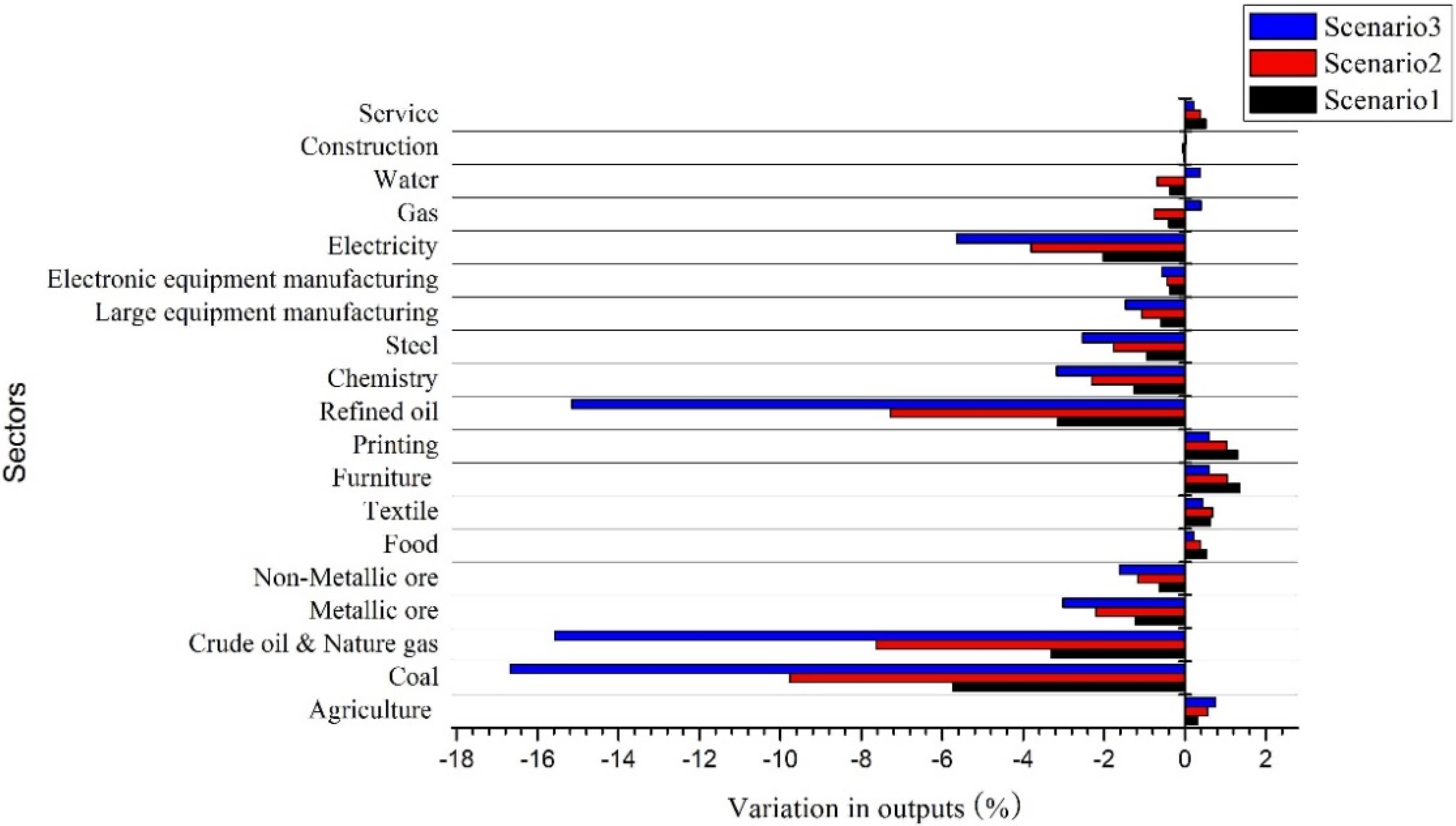
Figure 4. Change of industry level output in Scenario 1, Scenario 2 and Scenario 3.

Figure 4. Change of industry level output in Scenario 1, Scenario 2 and Scenario 3.

In Figure 4, there are changes of output in each industry after levying the environmental tax. As we mentioned above, the biggest drop appeared in enterprise revenue, so it is necessary to analyze the changes at an industry level.

Simulation results show that the vast majority of the industries suffer negative impacts and the extent of impacts are proportional to the emissions intensity. The five kinds of energy industries suffer great output losses, and other high-emission industries such as chemicals, steel, the manufacturing industry, and the selection, smelting and processing of mineral products also experience sharply declines of outputs. In addition, with the increase of tax rate, the extent of the decline shows an increasing trend.

What is noteworthy is that not all the industries’ outputs drop, for example food, service, agriculture, furniture and so on. Their outputs show an increasing trend rather than a sharp drop.

4.2. The Simulation Results of Different Tax Refund

This part shows the results of different tax refunds, including the impacts of the environmental tax on the macroeconomic variables and the impacts on industry levels. The results are reported in Table 3 and Figure 5. In Table 3, most of macroeconomic indexes also decline, but in the Scenarios 5 and 6, the losses of most macroeconomic indexes such as GDP, enterprise revenue, enterprise savings and so on are relatively smaller than in Scenario 4. In Scenarios 5 and 6, the inhabitant consumption increases slightly, the government revenue decreases remarkably and the government expenditure experiences a decline compared to Scenario 4. What’s more, the emission reduction effects are weakened, and the ratio of emission reduction is decreased. For example, the decreases of CO₂ in Scenarios 4–6 are 9.64%, 7.33% and 8.27%, so obviously, the worst emission reduction appears in Scenario 5. As for the reasons, we will discuss them later.

Table 3. The impacts of different environmental tax refund methods on macroeconomic variables.

Index	2010			2020
	Scenario 4	Scenario 5	Scenario 6	Scenario 4	Scenario 5	Scenario 6
Macro-Economic Indexes (%)
GDP	−0.805	−0.312	−0.463	−0.604	−0.285	−0.325
Inhabitant consumption	0.159	0.279	0.186	0.068	0.132	0.086
Investment	−0.364	−0.037	−0.198	−0.318	−0.022	−0.09
Exports	−0.512	0.124	0.234	−0.509	0.236	0.2
Imports	−2.603	−2.132	−1.541	−2.603	−2.024	−1.378
Inhabitant income	0.159	0.279	0.186	0.068	0.132	0.086
Enterprise revenue	−3.472	−1.579	−1.902	−2.602	−1.385	−1.744
Enterprise saving	−3.136	−1.212	−1.368	−3.136	−1.367	−1.142
Government revenue	9.523	1.148	0.901	8.068	0.589	0.685
Government expenditure	0.483	−0.237	−0.261	0.450	−0.128	−0.234
Emission Reduction Effect (% Decreased Amount)
CO2	9.642	7.326	8.271	8.797	7.132	7.871
SO2	8.569	7.013	7.681	7.364	6.724	7.042
NOx	7.284	6.582	6.951	6.978	6.013	6.751
CO	9.234	7.241	8.032	8.262	7.182	7.679

Table 3. The impacts of different environmental tax refund methods on macroeconomic variables.

Index	2010			2020
	Scenario 4	Scenario 5	Scenario 6	Scenario 4	Scenario 5	Scenario 6
Macro-Economic Indexes (%)
GDP	−0.805	−0.312	−0.463	−0.604	−0.285	−0.325
Inhabitant consumption	0.159	0.279	0.186	0.068	0.132	0.086
Investment	−0.364	−0.037	−0.198	−0.318	−0.022	−0.09
Exports	−0.512	0.124	0.234	−0.509	0.236	0.2
Imports	−2.603	−2.132	−1.541	−2.603	−2.024	−1.378
Inhabitant income	0.159	0.279	0.186	0.068	0.132	0.086
Enterprise revenue	−3.472	−1.579	−1.902	−2.602	−1.385	−1.744
Enterprise saving	−3.136	−1.212	−1.368	−3.136	−1.367	−1.142
Government revenue	9.523	1.148	0.901	8.068	0.589	0.685
Government expenditure	0.483	−0.237	−0.261	0.450	−0.128	−0.234
Emission Reduction Effect (% Decreased Amount)
CO2	9.642	7.326	8.271	8.797	7.132	7.871
SO2	8.569	7.013	7.681	7.364	6.724	7.042
NOx	7.284	6.582	6.951	6.978	6.013	6.751
CO	9.234	7.241	8.032	8.262	7.182	7.679

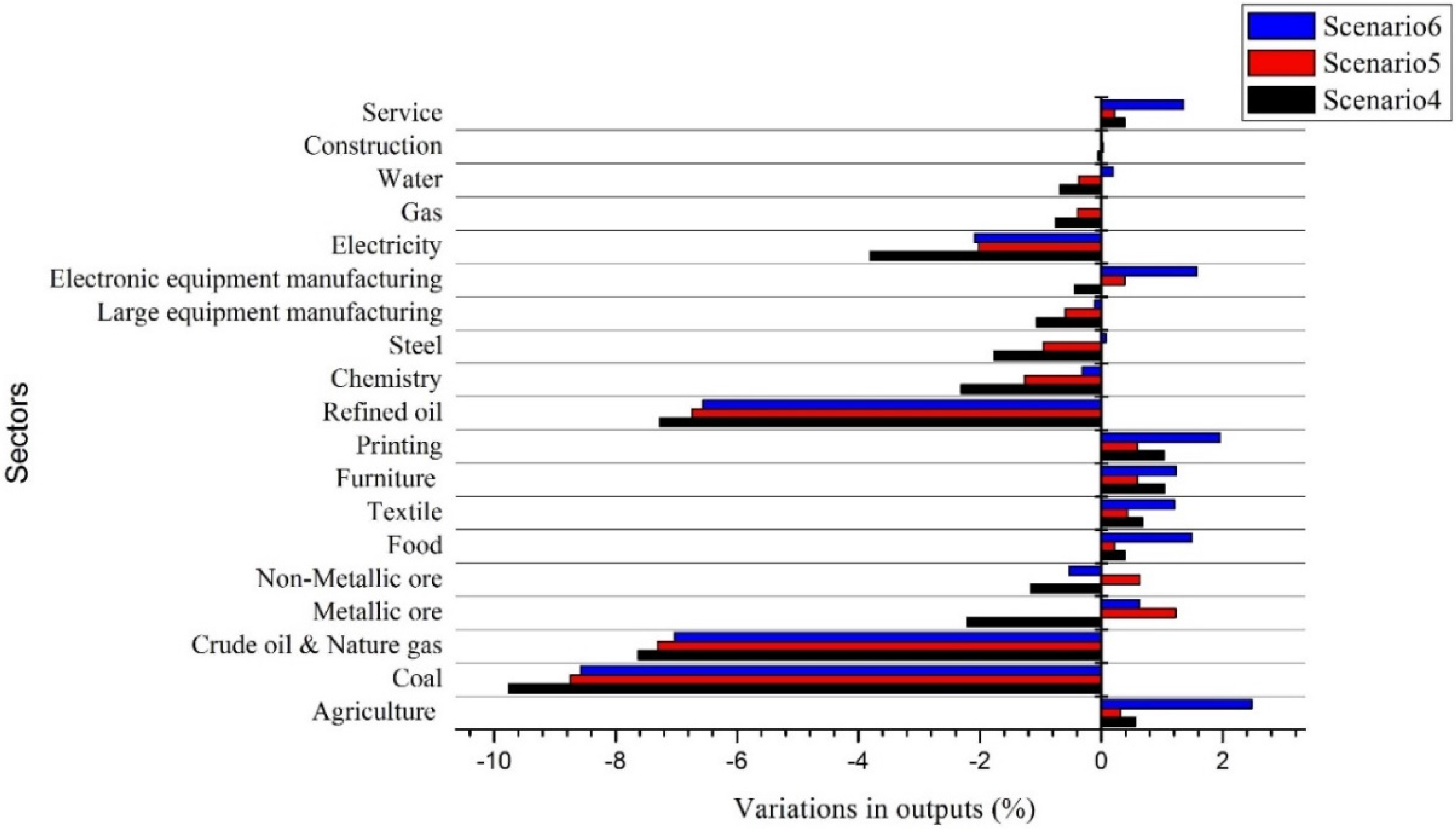
Figure 5. Change of output at the industry level in Scenario 4, Scenario 5 and Scenario 6.

Figure 5. Change of output at the industry level in Scenario 4, Scenario 5 and Scenario 6.

In Figure 5, there are changes of output in each industry with different tax refund methods. The simulation show that a vast majority of the industries suffer negative impacts and the energy sectors still suffer great output losses. In Scenarios 5 and 6, the losses in most energy-intensive sectors are smaller than in Scenario 4. It is worth noticing that some sectors such as service, food, furniture and so on which have rising outputs without tax refunds have significant output increases in Scenario 6. Additionally, the simulation results show that there are still differences in the different tax refund methods.

5. Discussion

5.1. Discussion of Different Tax Rates

5.1.1. Impacts on Macroeconomic Variables

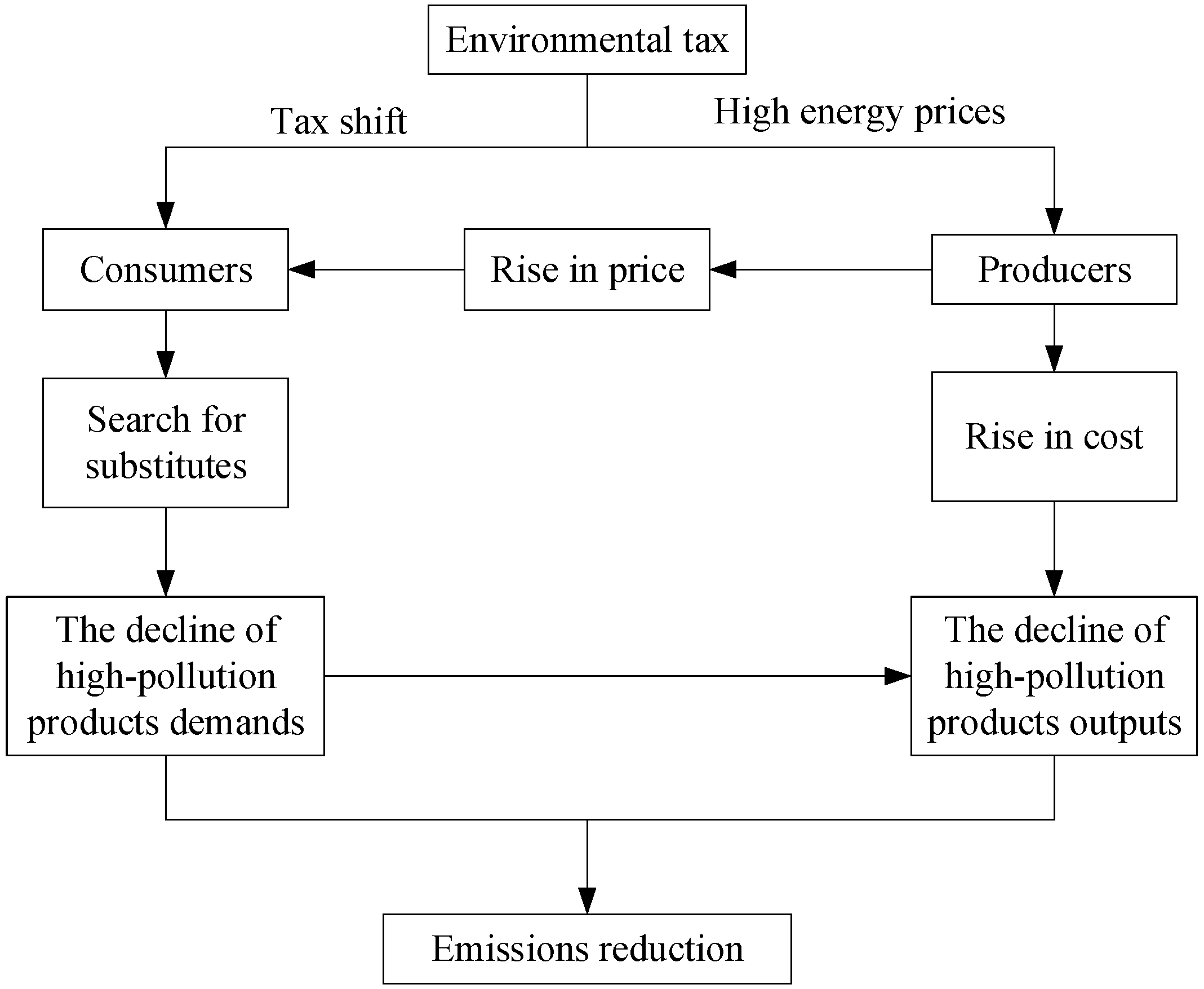
Needless to say, the environmental tax will affect the market mechanisms especially the demand-supply mechanism and price mechanism, which are both key factors to determine the market equilibrium. Price conduction mechanism means that the market price is influenced by many factors, and these factors can interact with relative prices in a certain way. The highly articulated price chain presents an organic connection of commodity prices, which means any change in the price chain will transfer to other parts through cost-push or demand-pull. The environmental tax is an indirect tax, in accordance with the tax shifting and price conduction mechanism, a tax imposed upstream will transfer downstream through cost-push. For example, if the environmental tax is imposed on the coal sector, the price of coal will increase. The higher coal price will lead to a rising cost for power generation enterprises and the electricity price shall increase accordingly. Obviously, electricity is a basic necessity in production and residents’ life, so the rise in electricity price will inevitably give rise to a rise in the price levels in the whole society. The environmental tax will cause a series of chain reactions just like we mentioned above, and all these changes will lead to the changes in the macroeconomic environment, such as the loss in GDP, the decline in enterprise revenue and so on. The environmental tax transmission mechanism is shown in Figure 6.

Figure 6. Transmission of the environmental tax in the economy.

Figure 6. Transmission of the environmental tax in the economy.

Given the broad effects and impact scopes of levying the environmental tax, the behaviors, such as consumption, investment, and saving of three economic subjects are the things that we most care about:

(1)

GDP

Regarding the GDP, the core index of national economic accounting, the impacts of environmental tax shows negative effects on it; fortunately, the negative effects are not as strong as we predict. Under Scenarios 1–3 in 2010, the impacts of environmental tax of the three levels on GDP are −0.46%, −0.81%, and −1.27%. Even levying the high level of tax, the GDP fluctuation still remains in a relatively small range. In the long run, the negative effects on GDP show a decreasing trend, in the same scenario but different year, the negative effects on GDP are much lower in 2020 compared to the initial impacts in 2010.

(2)

Inhabitant Behavior

The consumption of inhabitants increases by a small margin, meanwhile, the income of inhabitant increases slightly. In Scenarios 1–3 in 2010, the increases of consumption are 0.04%, 0.16%, and 0.14%, and the increases of income are 0.04%, 0.16%, and 0.14%. As we all know, levying an environmental tax can reduce the GDP, which means the economy is contracting, thus this can lead to falling revenues. Furthermore, the deterioration of trade terms also leads to an income decrease. Why does the income increase rather than decrease? Although the wage income of inhabitants is decreased by the shrinking labor demand, the government income will increase, thus the transfer payments from the government to inhabitants will increase.

As for inhabitants’ consumption, the increases of consumption are caused by the rising prices rather than increasing demand. Under the condition of unchanged living consumption, the rising prices will lead to an increase of living costs, but in Scenario 3 the increment of consumption is smaller than Scenario 2, mainly because the high level tax causes a substantial growth in commodity prices, so the inhabitants have to cut their demand.

(3)

Enterprise Behavior

Enterprises are the biggest economic subjects among the three subjects, so the environmental tax will exert significant impacts on enterprises. Under Scenarios 1–3 in 2010, the enterprise revenue decreases sharply by 1.86%, 3.47%, and 5.12% respectively. After introducing the environmental tax into the economy, the enterprises, especially the carbon-intensive industries, suffer a lot of direct shock from the policy.

The downtrend of output level in each production department can be interpreted by the principle of equilibrium price: the equilibrium output and equilibrium price are determined by the interaction between supply and demand. On the one hand, the environmental tax raises the energy cost of the production department, so that the supply decreases. On the other hand, the environmental tax also reduces the demand for high-polluting energy, however, the change of the demand for energy affects the equilibrium output and equilibrium price of the energy sector, and also affects the production cost of other production departments. Finally, market equilibrium is accomplished by the linkage effect between price and output, and most of the enterprises’ outputs decreased.

(4)

Government Behavior

The government benefits from the environmental tax. Under Scenarios 1–3 in 2010, the government revenue increases by 4.98%, 9.52%, and 15.28%, respectively, and the government expenditures increase by 0.26%, 0.48%, and 0.72%. In these three scenarios, the government imposes the environmental tax without tax refunds, and environmental tax is retained as part of the government’s budget. Although the government obtains considerable revenue, it is not conducive to economy operation. The benefit maximization is not the aim of the government, it should, and even must reduce the impacts of the environmental tax via fiscal and monetary policy, which we will discuss later.

(5)

Investment

The investment drops in all scenarios. Under Scenarios 1–3 in 2010, the investments decrease by 0.20%, 0.36%, and 0.90%, respectively. When levying an environmental tax, most industries may be adversely affected, especially high energy-consuming and carbon-intensive industries. These industries tend to be more capital-intensive than their low-emission peers. The decline of capital stock results in investment decline, which also contributes to a decline in GDP.

5.1.2. Impacts on Industry

After analyzing the macroeconomic variables, we will analyze the impacts of the environmental tax on each production department. The subdivision of industry enables us to understand the impacts of the policy transmission mechanism at the industry level. The output variations in three scenarios are shown in Figure 4. Simulation results show that the vast majority of the industries suffer negative impacts and the extent of impacts are proportional to their emissions intensity.

Theoretically, levying an environmental tax will increase the cost of energy, and the rising cost will pass on to consumer in the form of higher prices, and high prices will in return suppress consumption. Thus, a series of changes contribute to the decreases of output in the energy department.

In addition, the energies whose elasticity demands are small have low substitutability, and some production departments have no choice but accept the high prices of energy, which will lead to higher prices of their output. Therefore, the decreases of outputs not only occur in the energy sectors, but also occur in the energy-intensive industries as well, such as metallic and non-metallic ore, manufacturing, steel, chemicals and so on.

It is interesting to notice that not all industries suffer a decline of outputs, for example agriculture, tertiary industries, and light industries. On the contrary, the outputs of these industries increase rather than decrease. The main reason is that the demand of energies in these industries are lower than those of the heavy industries, and they can also substitute the low emission energies for high emission energies.

Will all high-emission industries suffer great outputs losses? No, such as the case of electricity. Compared with coal, oil and natural gas, the electricity industry has its particularity. In China, thermal power accounts for about 75% m of the production, that is, electricity generation will cause high emissions, but its output decline is relatively small. In this paper, we follow the principal “the polluter pays”. The end-use of electricity is zero emission, thus, the price of electricity is lower than that of other energies and some industries substitute electricity for other energies.

5.2. Discussion of Different Tax Refund

With the increasing tax rates, most of the macroeconomic variables are adversely affected. Obviously, without the complementary methods, the negative market impacts would be serious and broad-based. Therefore, it is necessary for government to use fiscal policy to help the market adapt to the changes caused by an environmental tax.

5.2.1. Impacts on Macroeconomic Variables

(1)

GDP

With respect to the GDP, the GDP loss under Scenario 6 (−0.46%) is only about half of that under Scenario 4 (−0.81%). Compared to Scenario 6 where the corporate income tax is deducted, the GDP shock is slightly reduced if the tax revenue is used to deduct the production tax (−0.31%). It could be interpreted that tax refunds can stimulate consumption and other behaviors to offset some negative impacts.

(2)

Investment

The most obvious change took place in investment, which mainly contributes to the growth of GDP. As we explained above, the recipients of the impacts are production departments, especially capital-intensive industries, and the tax refund can stimulate capital investment, and then the increase of capital will lead to rising outputs. However, these two kinds of tax reduction have remarkably different effects, and compared to Scenario 6 (−0.20%), the investment loss under Scenario 5 (−0.04%) is only one fifth.

(3)

Enterprise behavior

In terms of enterprise revenue, the two kinds of tax refund will exert a marked influence, so we analyze them emphatically. Under Scenarios 4–6 in 2010, the enterprise revenue decreased by 3.47%, 1.58%, and 1.91%, respectively. Scenario 4 is the base scenario without tax refund, in which the negative impacts are highest compared with Scenarios 5 and 6. Refunding the environmental tax to enterprises can reduce the additional cost so that the commodity prices will decline, then the lower prices will stimulate inhabitant consumption. Although it cannot completely offset the negative effects, the chain reaction will at least lead to an increase of enterprise revenue. It is obvious that there still exist different effects between the two kinds of tax refund methods, and the difference is what policymakers should focus on. Production tax includes added value tax, business tax and so on, which covers the entire production process. In other words, the production tax covers a broader tax base than the corporate income tax, thus, the impacts of deducting the production tax are bigger than deducting the income tax. The former can offset more negative effects in the enterprise revenue.

(4)

Government behavior

Because the government refunds the environmental tax, both the government revenue and government expenditure are greatly decreased compared with Scenario 4. That is, the government sacrifices its welfare to make up the negative effects exert by an environmental tax.

(5)

Emission

If the tax revenue is recycled to deduct the production or income tax, the emission reduction effects still exist, but no matter what refund method is used, the emission reduction effects will slightly drop compared with Scenario 4. The tax that is refunded to enterprises has three purposes: (a) stimulate the technical reform of existing enterprises; (b) reduce the negative impacts on production departments, especially the energy-intensive departments; (c) promote a smooth structural transition. On the contrary, some enterprises prefer to cut production costs rather than reform their technology. This may lead to an increase of emissions. What’s more, the tax refunded to enterprises will lead to the decrease of prices and increase of outputs, which can also contribute to the increase of emissions.

5.2.2. Impacts on Industry

Similarly, we analyze the impacts on each department. The output variations in three scenarios are shown in Figure 5. It is obvious that most department outputs are affected adversely in these scenarios, especially the high-emission and energy-intensive industries. For the energy sectors, the coal sector still suffers the most and other energy sectors suffer from negative impacts too.

When we compare these scenarios, good growth momentum appears in Scenarios 5 and 6, and some industries such as agriculture, furniture, food, service and so on, most of which are low-emission industries, have positive responses. The tax refund can offset the rising costs caused by the environmental tax, and consequently stimulate the output of enterprises. The low-emission industries suffer less than high-emission industries, and their outputs even increase without the tax refund in Scenario 4, let alone when the government refunds the environmental tax. For those energy-intensive industries, although the outputs are still negative, the degree of negative impacts become smaller compared with Scenario 4. In other words, the refunded tax can offset part of the negative effects caused by an environmental tax in energy-intensive industries. The two kinds of tax refund have different effects, when the environmental tax is refunded to deduct the production tax, the positive effects are greater than deducting the enterprise income tax, which is in line with the macroeconomic variable changes.

5.3. Discussion of Dynamic Impacts

The results also show some dynamic impacts, and the details are shown in Table 2 and Table 3. The dynamic mechanism means that the model simulates the external shocks each year in the future according to the growth rate of capital and labor we set before, thus we can measure the impacts of environmental tax on economic market in the next few years. First, we analyze the dynamic impacts of different tax rates.

The majority of macroeconomic variables in Scenarios 1–3 are lowered in 2020 compared to the initial impact in 2010. However, the percentage deviations of these variables are different. The variables in Scenario 1 are close to the baseline, that is, the market can much easily accept a low environmental tax rate. That’s why the low-level tax rate should be introduced in the economic market. The markets are capable of regulating themselves, they can absorb relatively small external shocks, and adjust themselves by the market mechanism.

Regarding the inhabitant consumption, there are different levels of decline in all three scenarios in 2020. The reason might be that inhabitants can optimize their behavior due to the rising costs, they can adjust their consumption structure, replacing high-pollution commodities by low-emission commodities. In the long run, although the cost of living is rising, the consumption increment experiences a downward trend.

In addition, the industrial structure is progressively adjusted. Enterprises, like inhabitants, have behavioral optimization. With the rising cost, the demand for commodities produced by high energy-consuming and carbon-intensive industries decreases. Hence, the industrial structure gradually transfers to a low carbon-orientation. This also justifies the fact that the loss of enterprise revenue shows a decreasing trend in the long run.

The results also show some dynamic impacts of different tax refunds. Most variation trends are the same as the dynamic impacts of different tax rates, but there still exist some differences. In Scenarios 5 and 6, the GDP adjusts back to its baseline projection more quickly than Scenario 4, which means that the tax refund can help the market offset the external impacts. Additionally, the variations between 2010 and 2020 in enterprise revenue are much smaller than that in Scenario 4. The reason may be that the initial negative shock on the economic system is comparatively small in Scenarios 5 and 6 due to the tax revenue being recycled back to production departments which offsets the environmental tax shock a lot. Hence, the consequent dynamic impacts on enterprises are stable in the long run.

Although the tax refund may stimulate the outputs of enterprises, and the effect of emission reductions is affected, it is slightly lower in 2020 compared to the initial impact in 2010 in Scenarios 5 and 6. This implies that an environmental tax shock will extends its impact on emissions over a certain time period in China. This further confirms that an environmental tax is effective in reducing four kinds of pollutant emissions also from a time horizon perspective.

6. Conclusions and Policy Implications

As the environmental tax reform has been gradually put on the agenda in China, carrying out the study of environmental tax has become increasingly significant. In this paper, we studied the influence of an environmental tax on China’s economy through a dynamic recursive multi-sector CGE model, including the effects of different environmental tax rates and different tax refunds.

Our simulation results show that environmental tax is conducive to environment improvement but negative effects on macroeconomic variables appear simultaneously, such as the reduction of GDP, the decline of enterprise income and so on. A higher rate can result in a better emission reduction effect, but conversely cause more negative effects. Since levying an environmental tax would have negative impacts, so the question is whether if the government refunds the environmental tax will bring positive benefits? A finding derived from the simulation results shows that the tax refund can relieve the negative impacts, such as recovery in GDP and the stimulation of output in low-emission industries. Nevertheless, there are lower positive benefits in high-emission industries and energy sectors. What’s more, the increase of output will harm the emission reduction effect.

The simulation results also show the comparison between short run and long run. Although the negative impacts are relatively large in the short run, they will be weakened in the long run. The policy makers should not only focus on the short term, the long-term change should also be considered.

Although the effects of tax refunds are limited in China, it provides a new way of thinking, that is, combining the environmental tax with overall tax reform. This is conducive to achieve environmental protection, and can also reduce the negative impacts on the economy at the same time. In recent years, the Chinese government has been gradually promoting environmental tax reform, such as value-added tax relief, investment tax compensation, and import and export tariff preferences.

The determination of the best environmental tax rate is a burning question. The tax rate should cover pollution control costs at least, which can stimulate the reduction behavior of enterprises. However, this optimum tax rate is difficult to get. The policy makers should repeatedly adjust it after policy implementation. In addition, the marginal social cost of each pollutant in different regions is quite different. Therefore, it is necessary to establish a disparate tax rate system in accordance with the actual situation of different regions. What’s more, the four environmental taxes we considered have synergistic effects. The usage of a certain type of fossil fuel can cause multiple pollutants. e.g., the usage of coal can cause emissions of all four kinds of pollutants. Hence, the increase of a certain type of tax rate can also cause emission reduction of other pollutants. Needless to say, the environmental taxes have better performance than a single tax, but the balance between the environmental taxes is noteworthy.

Designing the environmental tax scheme would be a complex process. The current study is preliminary, and further work is required to improve the model. One of our future activities would be to further disaggregate the energy sectors with more available data, especially for clean energy and renewable energy. Moreover, the “double dividends” should be focused on. The first dividend, needless to say, it is easy to achieve, but no definite conclusions can be made about the second dividend so far because of the different backgrounds, economic structures, and systems in various countries. It is necessary to analyze the realization of “DD (Double Dividends)” in China.