
A Dynamically Adaptable Impedance-Matching System for Midrange Wireless Power Transfer with Misalignment

Abstract
:
1. Introduction
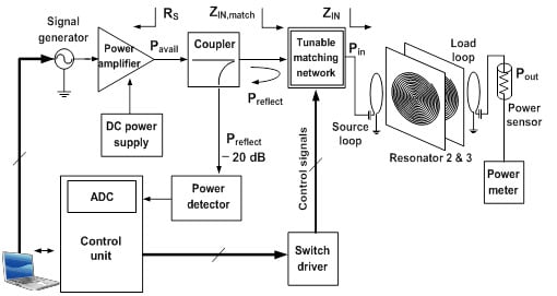
2. Design
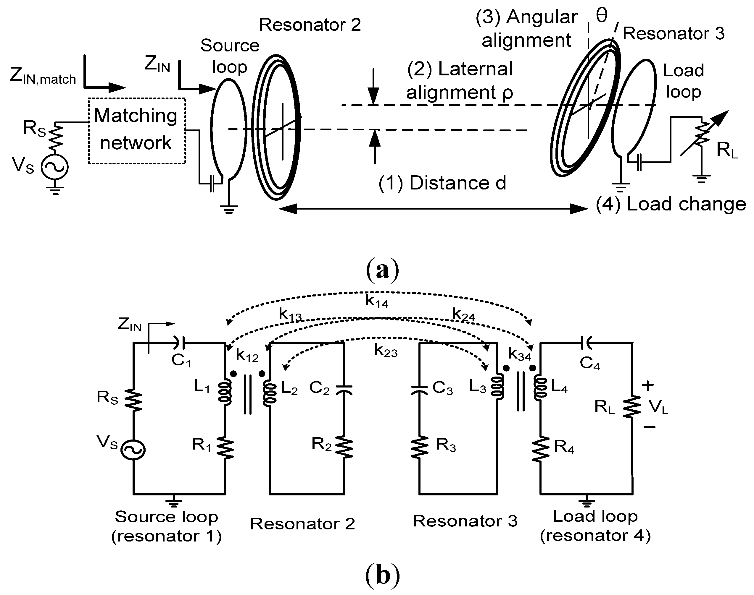
2.1. System Model

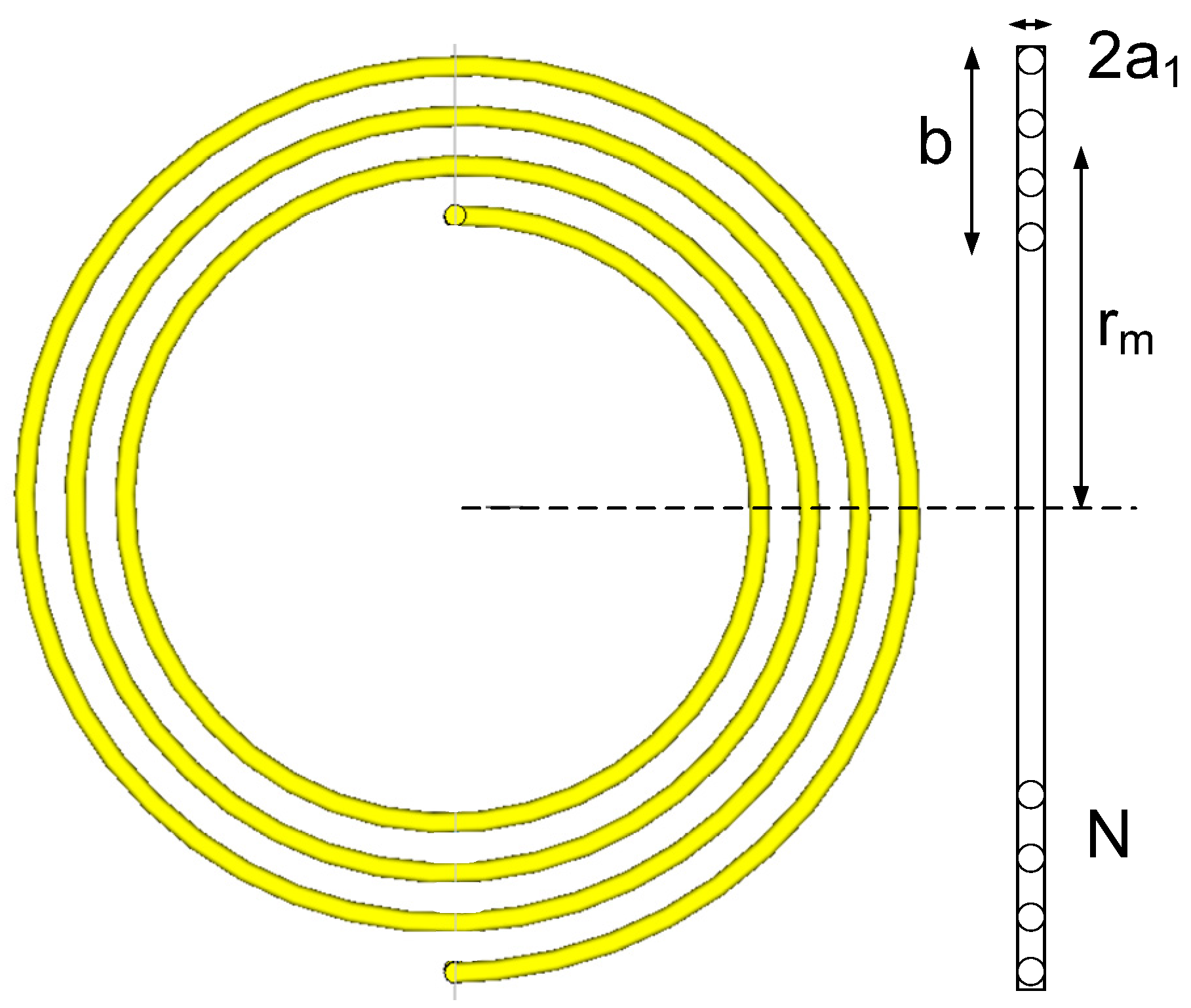
2.2. Parameter Extraction


| Parameters | Inductance (μH) | Resistance (Ω) | Resonant frequency (MHz) | Q factor @ f0 |
|---|---|---|---|---|
| Source loop | 1.33 | 0.5 | 6.75 | 113 |
| Resonator 2 | 40.1 | 5.5 | 6.76 | 311 |
| Resonator 3 | 39.5 | 5.2 | 6.78 | 324 |
| Load loop | 1.35 | 0.4 | 6.73 | 144 |
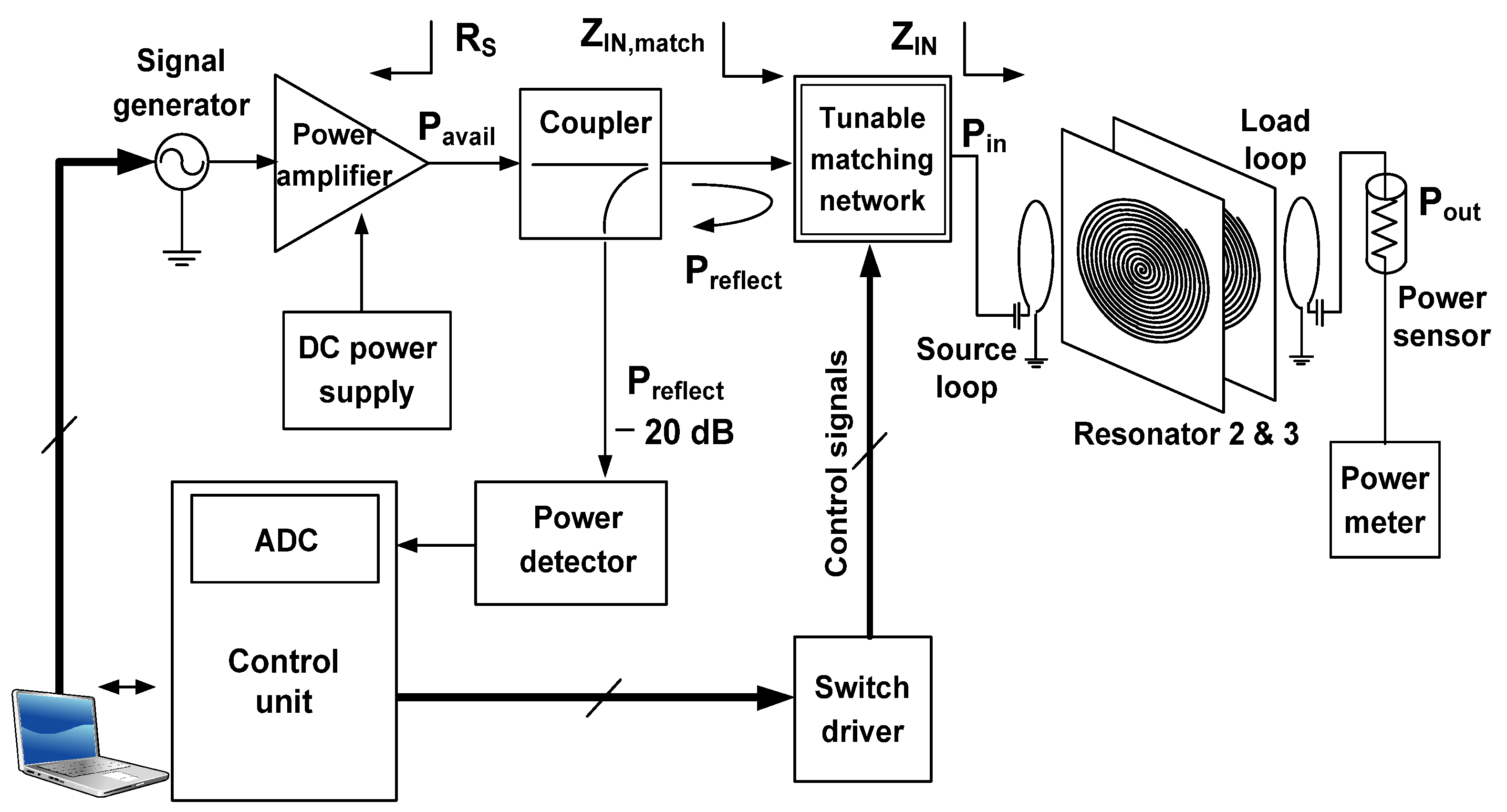
3. Implementation
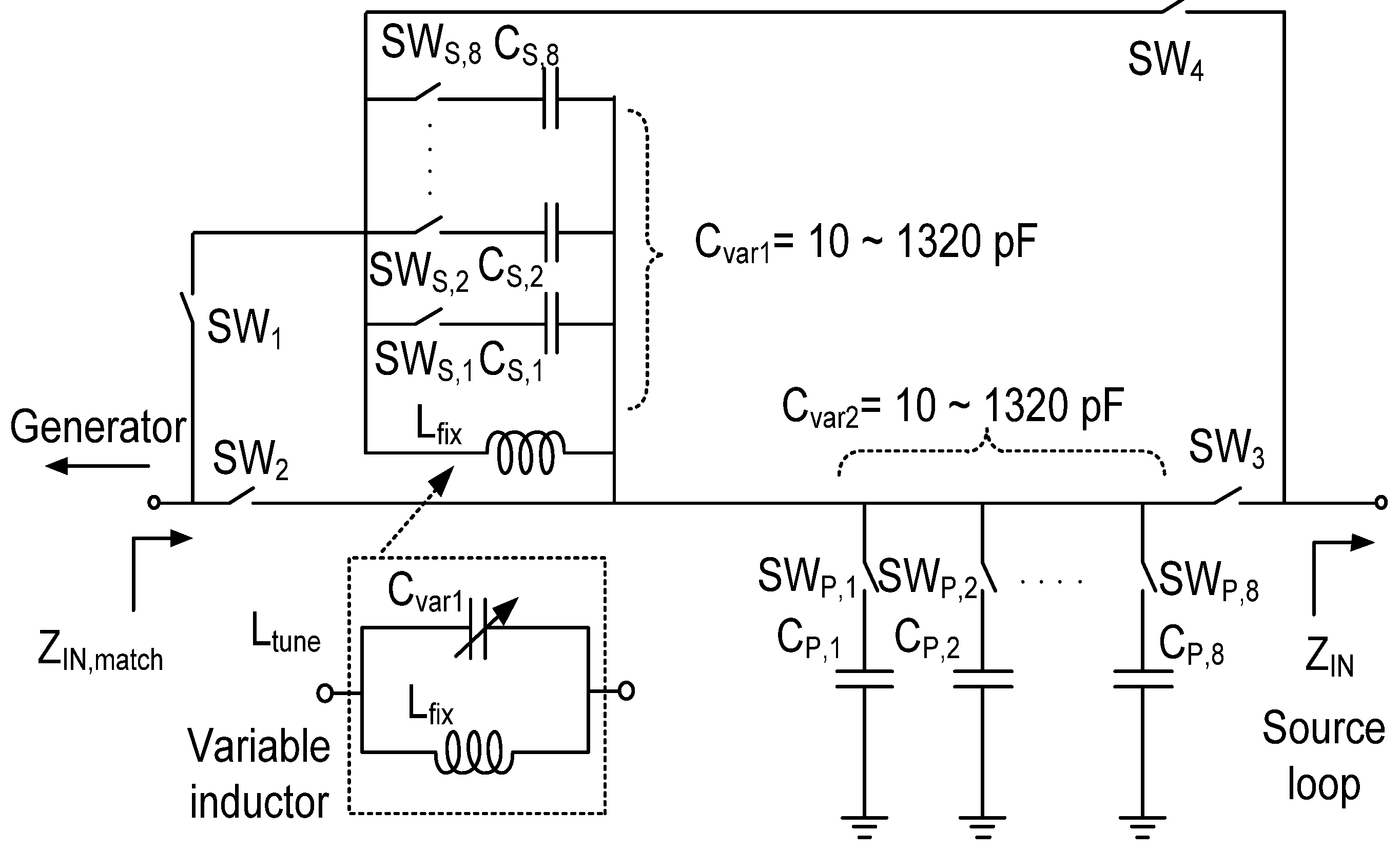
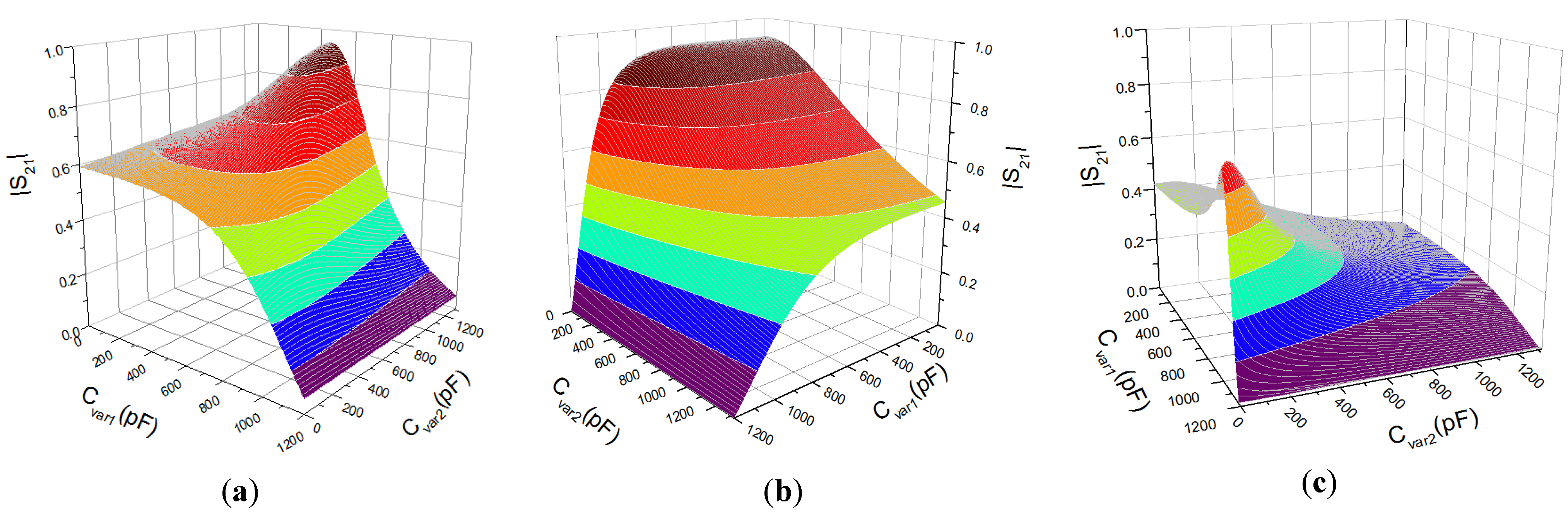
3.1. Tunable Matching Network


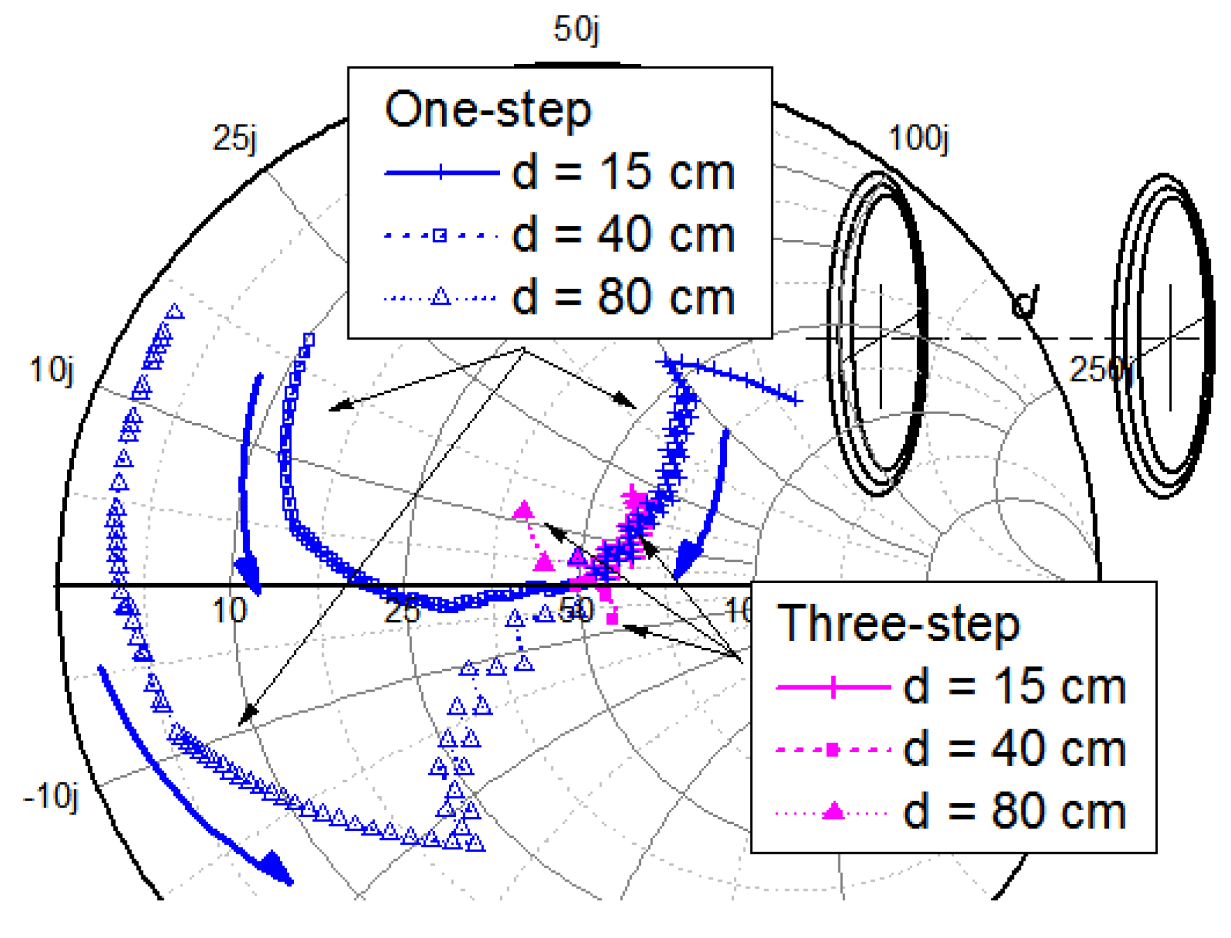
3.2. Three-Step Searching Method

- (1)
- Using the matching component values calculated in Step 2, set the initial starting point z(n,m) ϵ Z.
- (2)
- Add point z to the list of visited points L, or L = {z}.
- (3)
- Determine the set of eight neighboring points A(z) based on current location z.
- (4)
- Find the set of unvisited neighboring points R(z) using A(z) and list L.
- (5)
- Using the detected Preflect at the coupler, find the best matching point zopt among the eight neighboring points in R(z).
- (6)
- Check whether zopt remains unchanged. If yes, the system process ends. If no, add the already examined points R(z) to the list L; i.e., L = L U {z’| z’ ϵ R(z)}.
- (7)
- Assign new starting point z using local optimal point zopt for the next loop, and proceed to Step 3 (3).
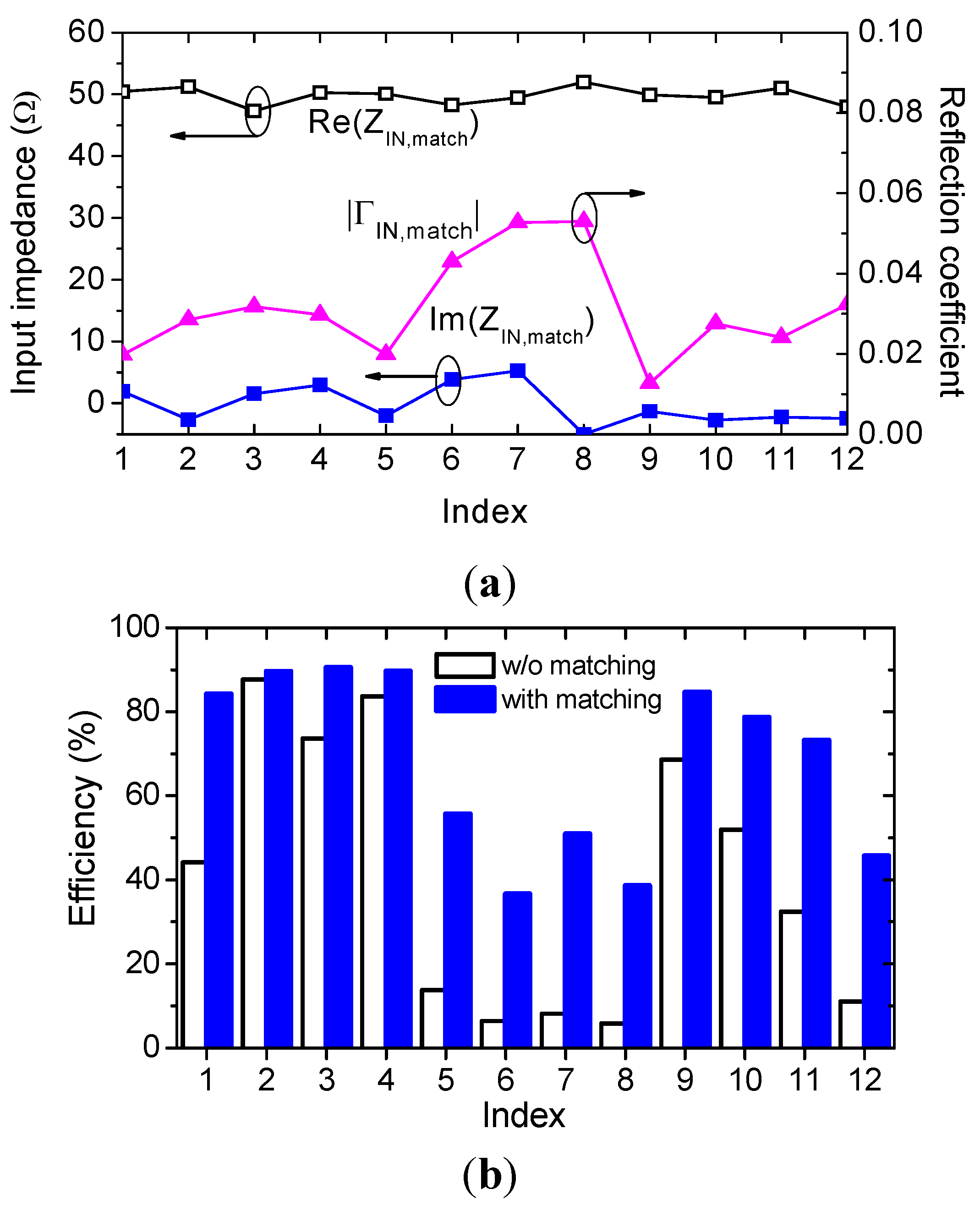
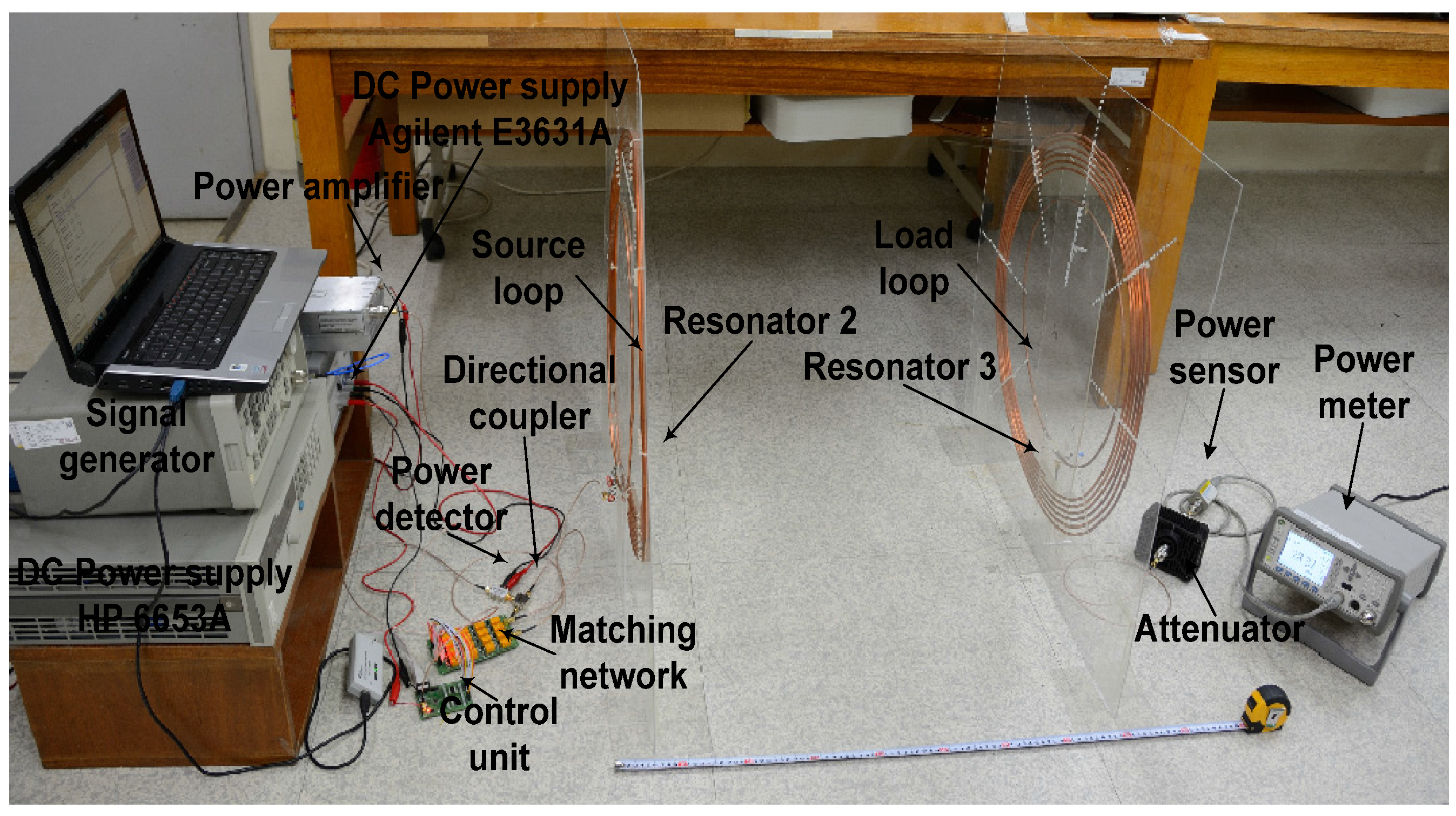
4. Experimental Results

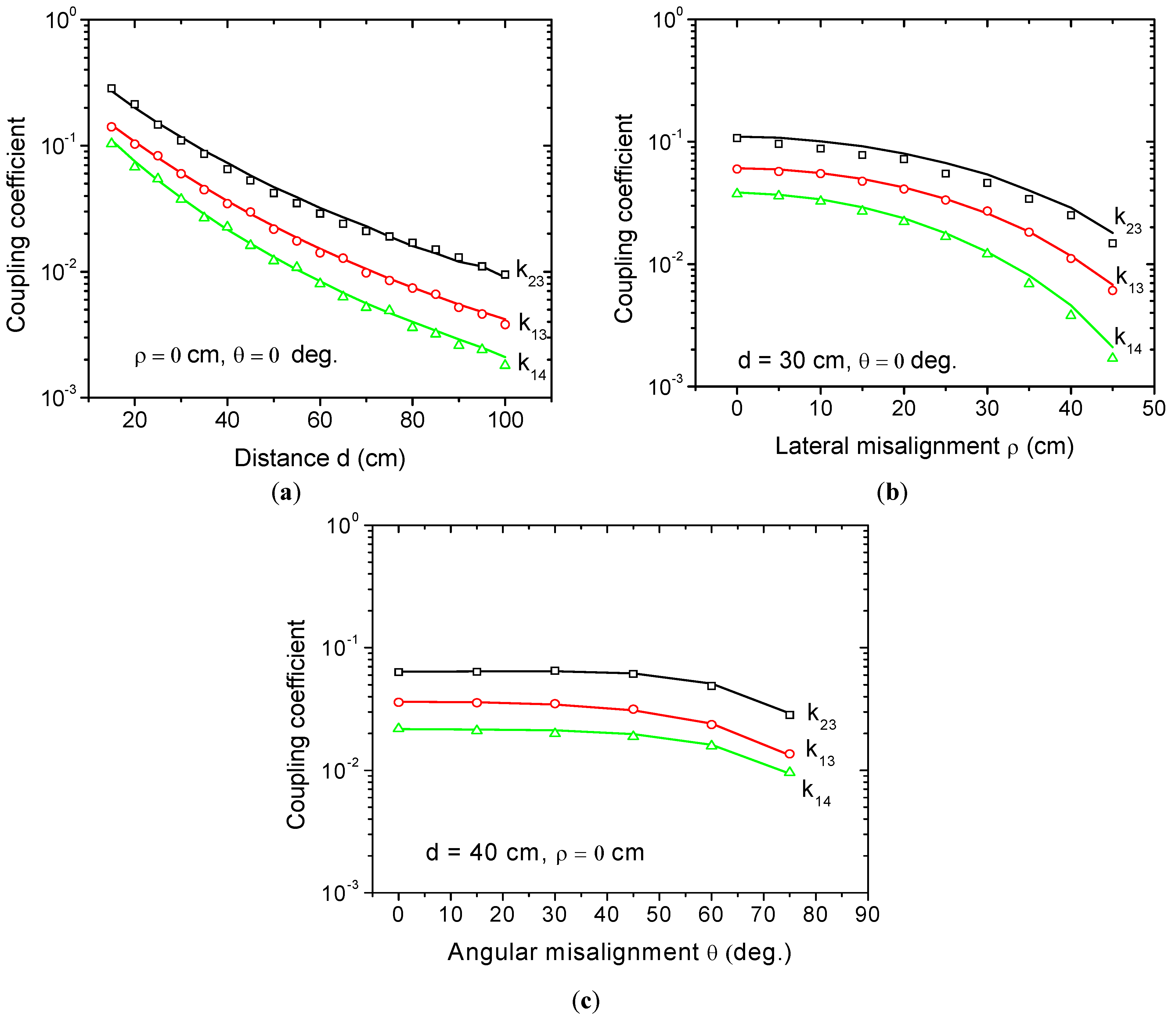
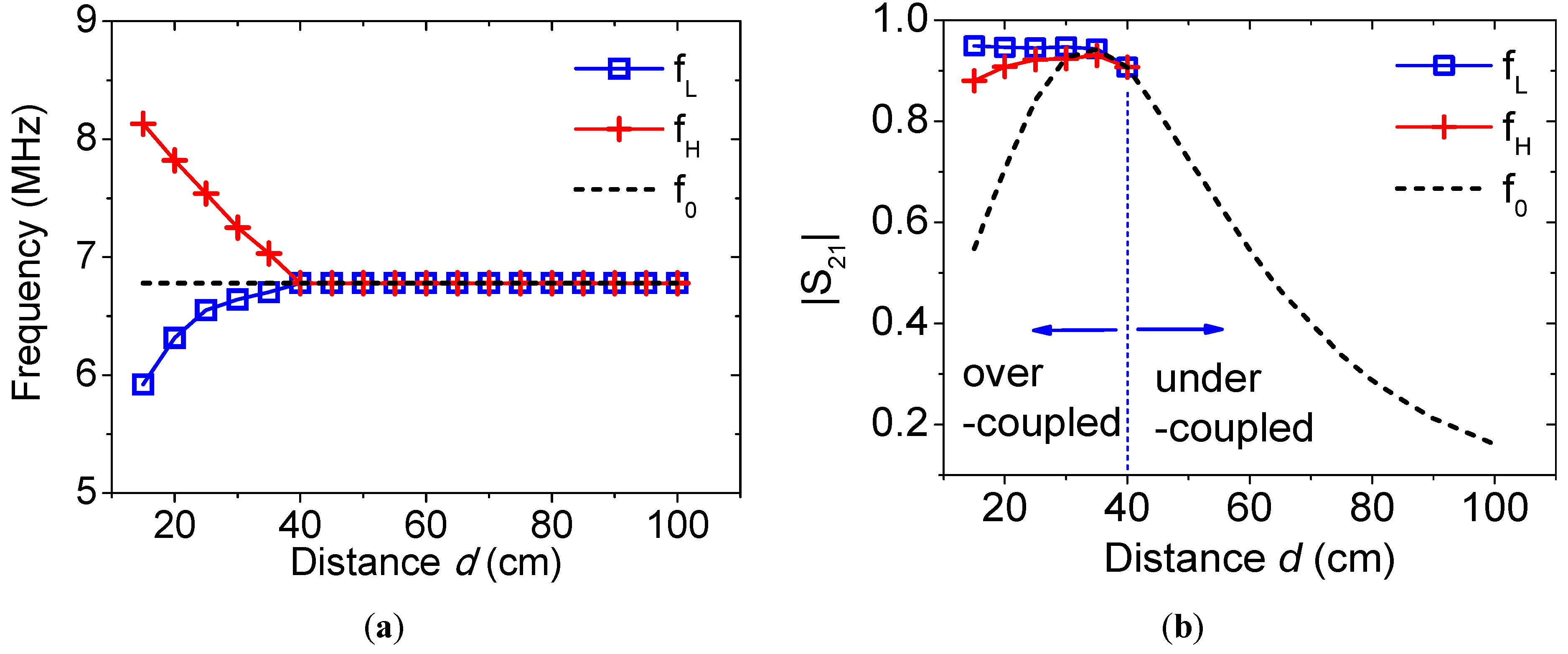
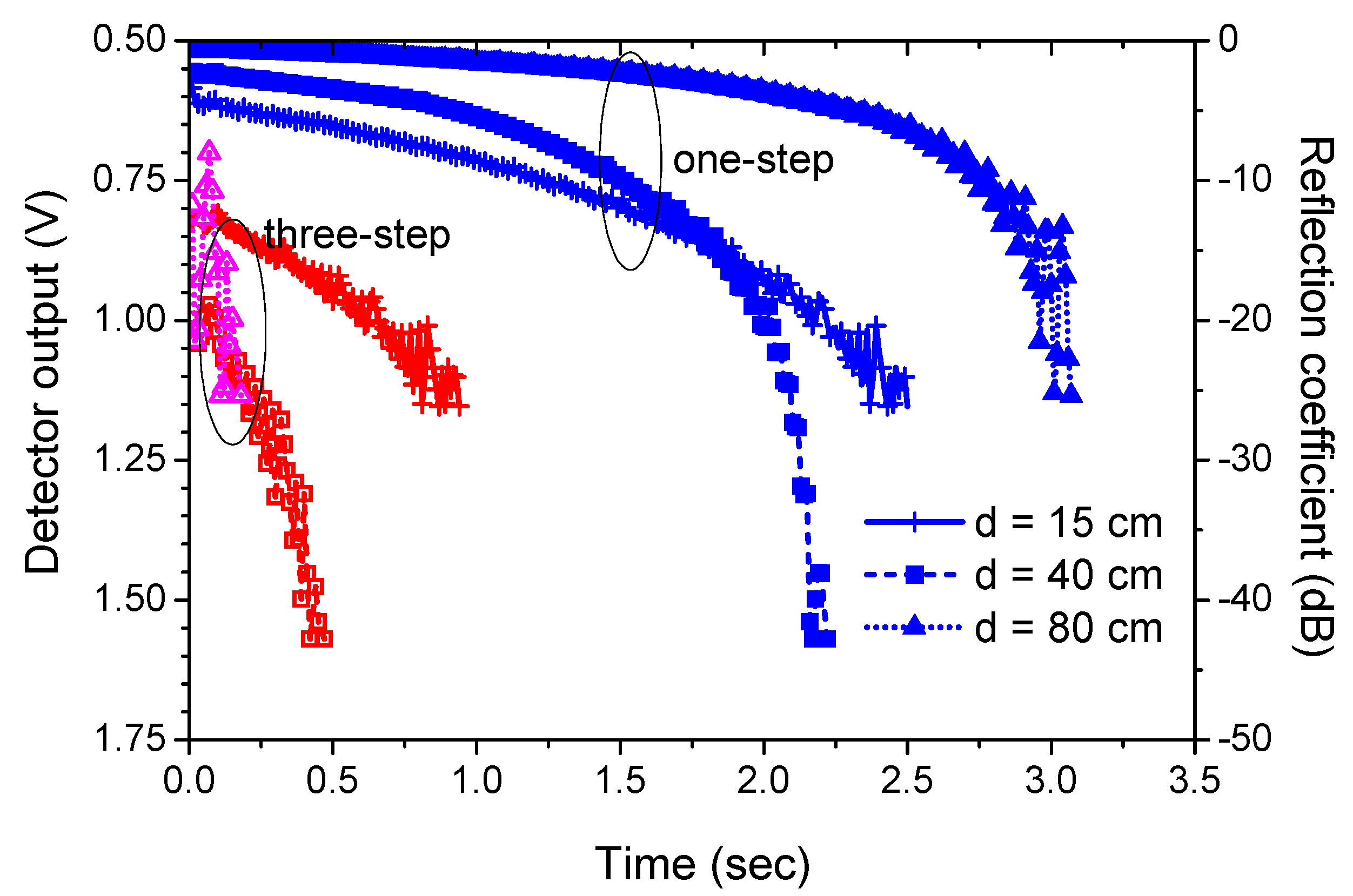
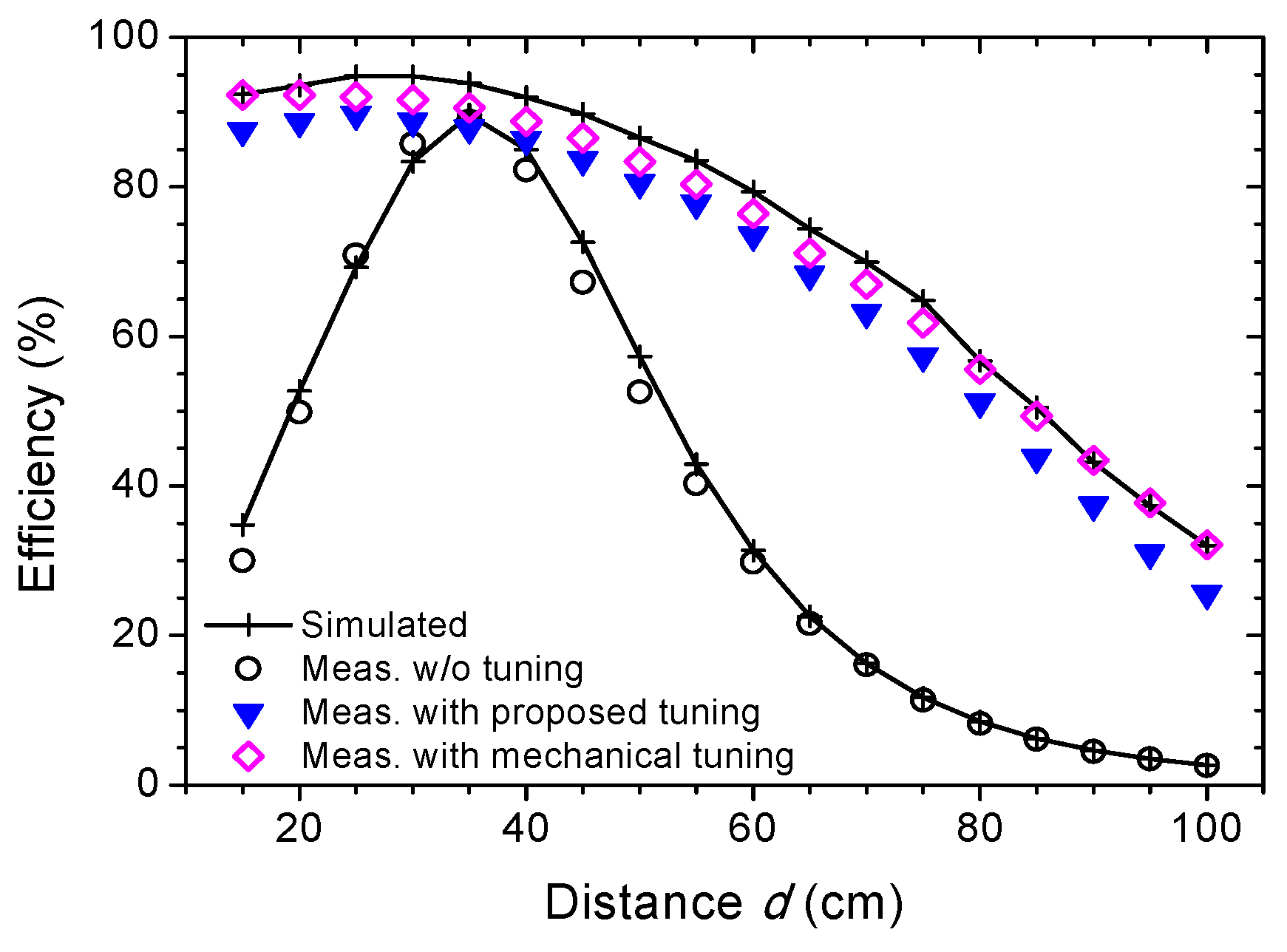
4.1. Distance Change

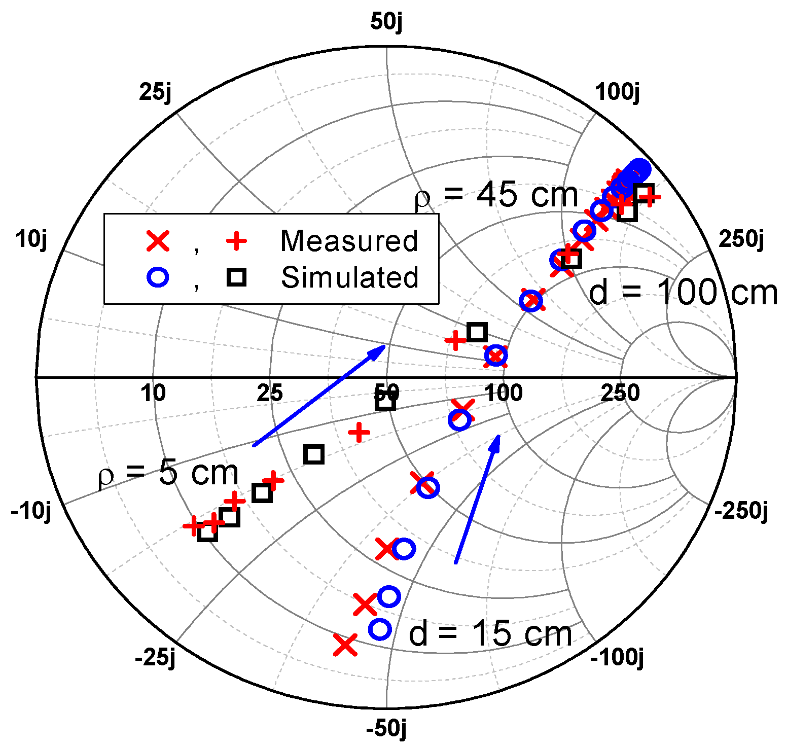
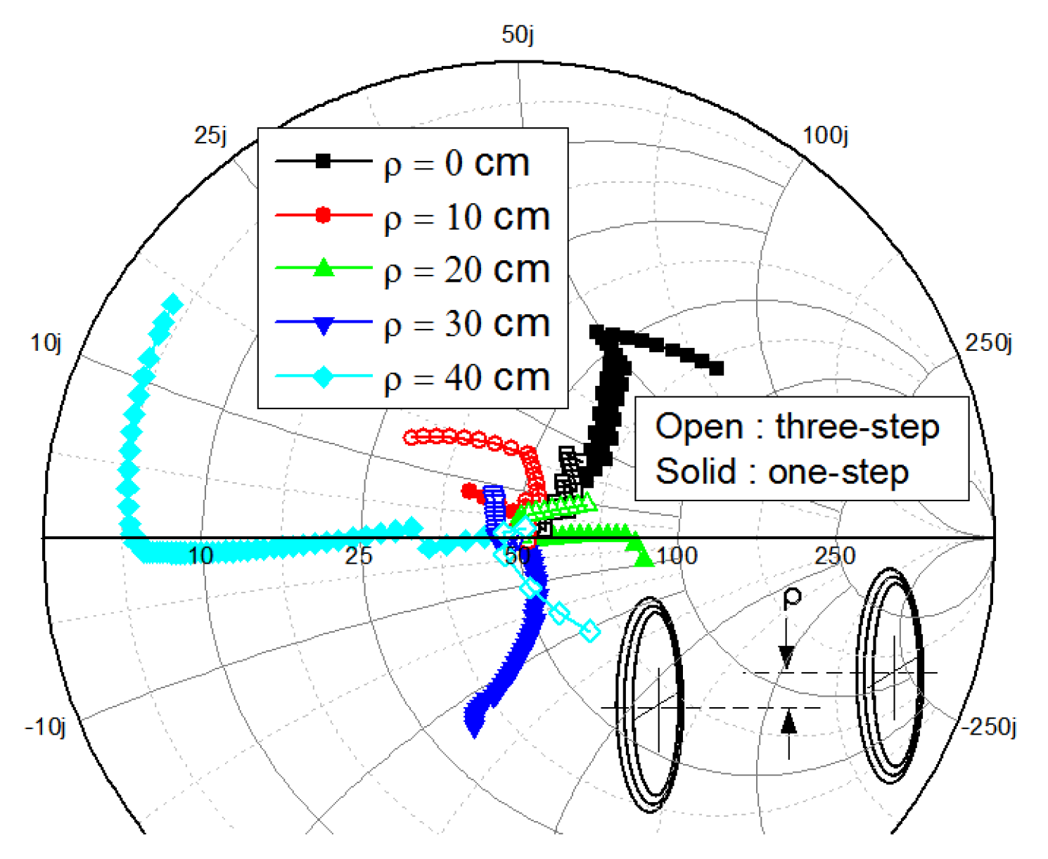
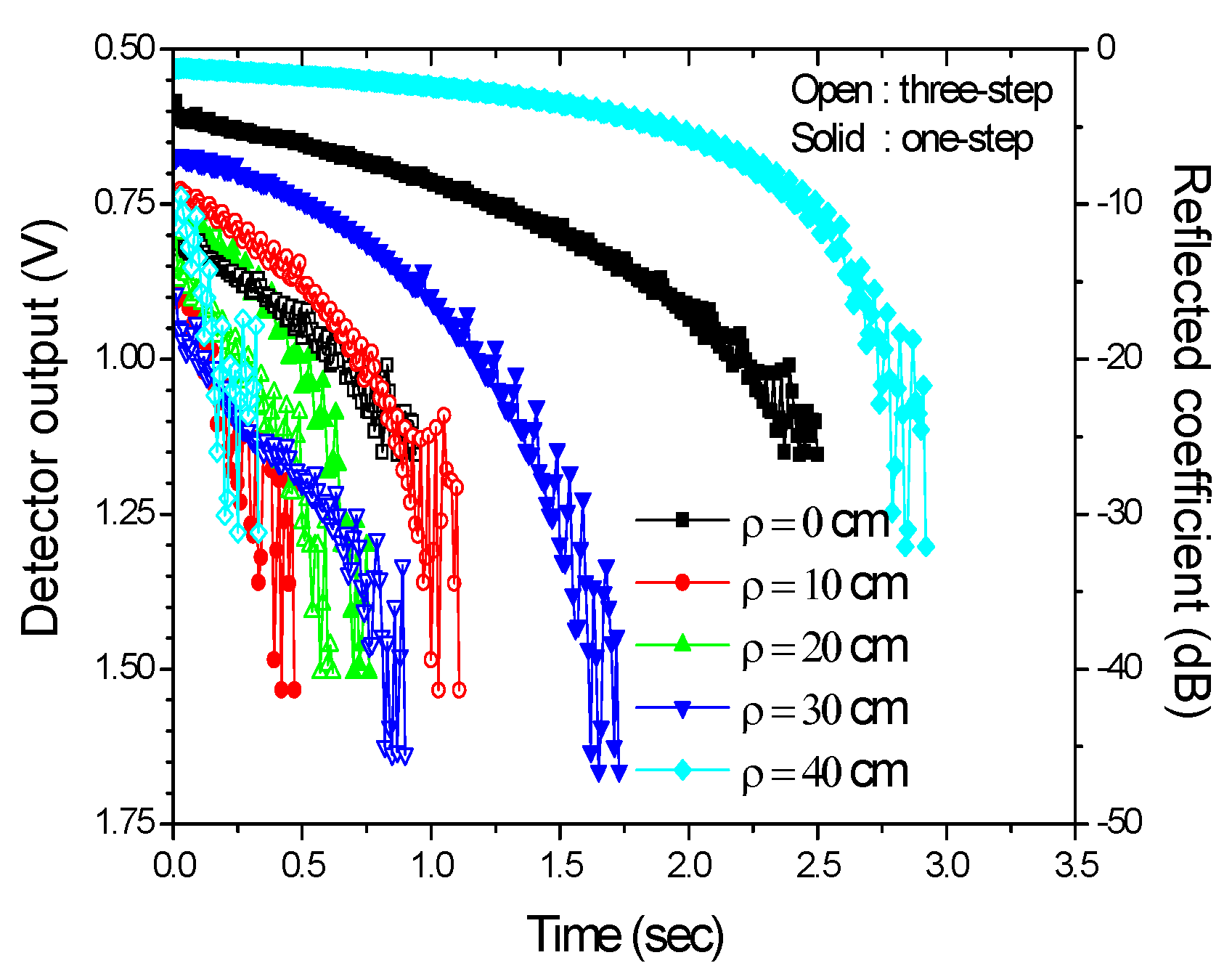
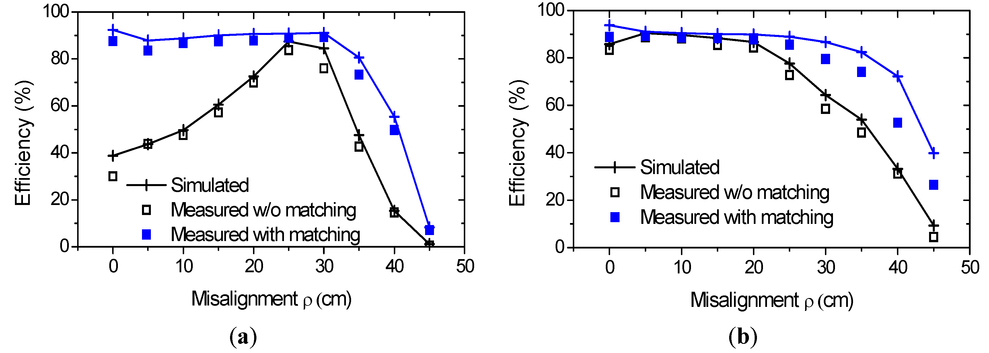
4.2. Lateral Misalignment

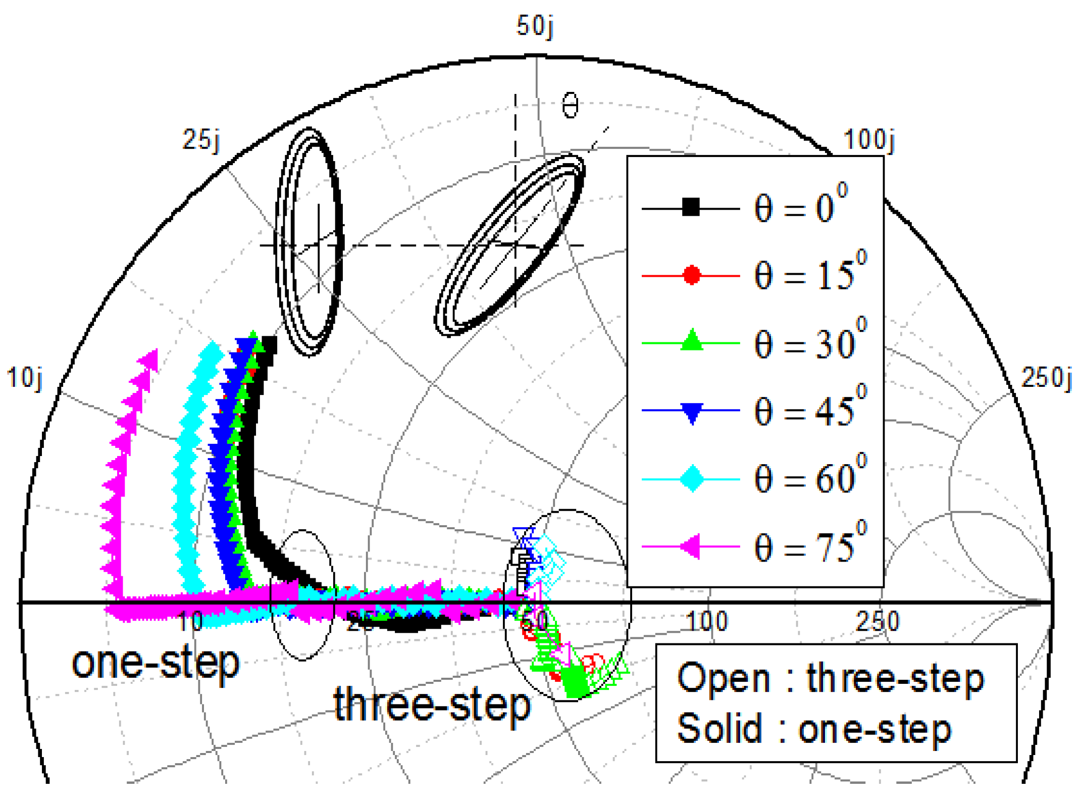
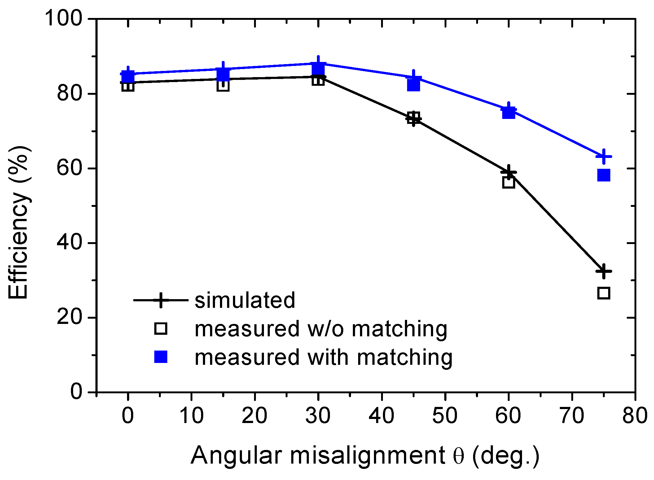
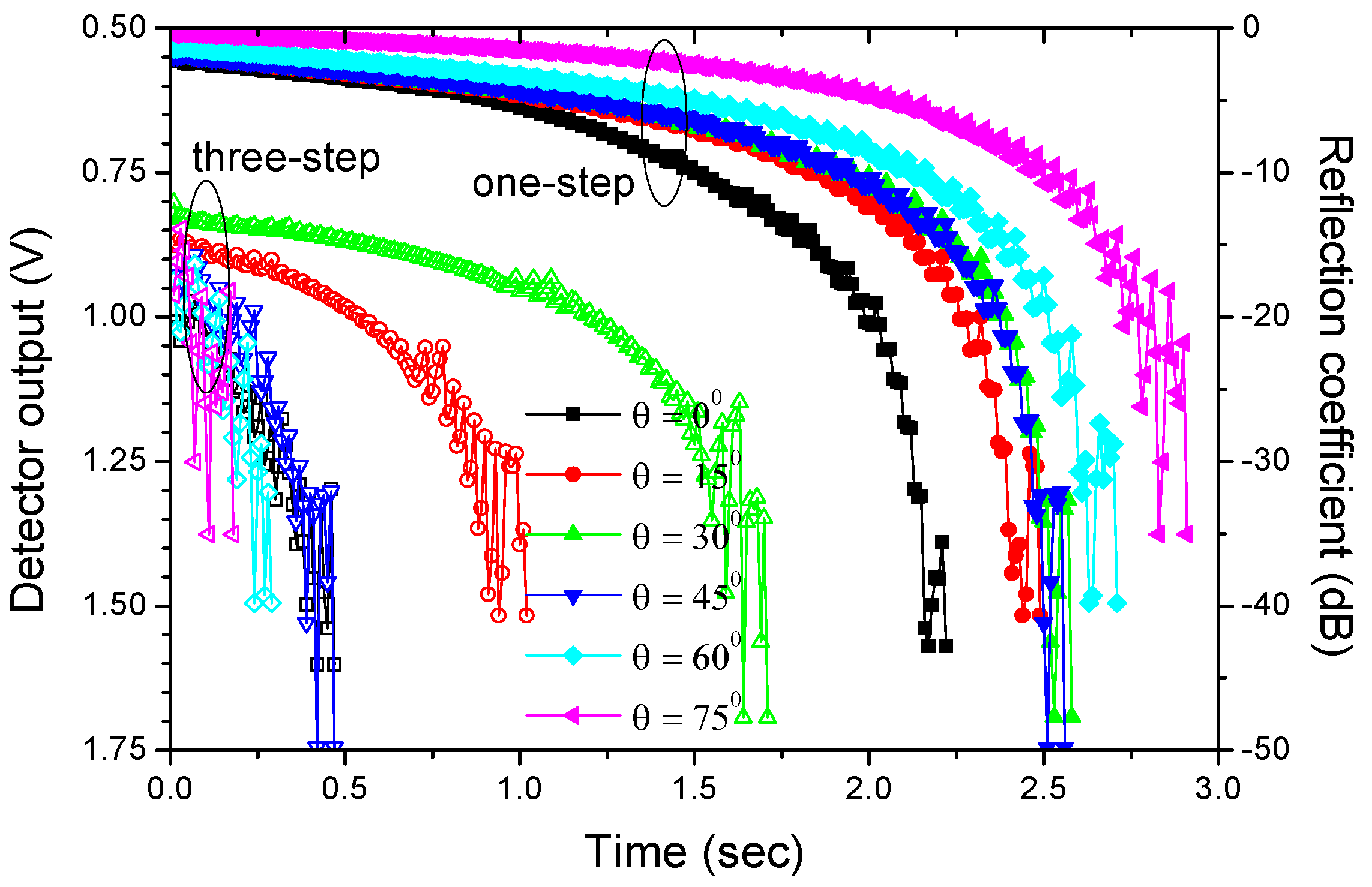
4.3. Angular Misalignment


5. Conclusions
Acknowledgments
Author Contributions
Conflicts of Interest
References
- Hui, S.Y.; Zhong, W.X.; Lee, C.K. A critical review of recent progress in mid-range wireless power transfer. IEEE Trans. Power Electron. 2014, 29, 4500–4511. [Google Scholar] [CrossRef]
- Wireless Power Consortium. Available online: http://www.wirelesspowerconsortium.com (accessed on 12 November 2014).
- Ahn, D.; Hong, S. A study on magnetic field repeater in wireless power transfer. IEEE Trans. Ind. Electron. 2013, 60, 360–371. [Google Scholar] [CrossRef]
- Rajagopalan, A.; RamRakhyani, A.K.; Schurig, D.; Lazzi, G. Improving power transfer efficiency of a short-range telemetry system using compact metamaterials. IEEE Trans. Microw. Theory Tech. 2014, 62, 947–955. [Google Scholar] [CrossRef]
- Ranaweera, A.L.A.K.; Duong, T.P.; Lee, J.W. Experimental investigation of compact metamaterial for high efficiency mid-range wireless power transfer applications. J. Appl. Phys. 2014, 116. [Google Scholar] [CrossRef]
- Kurs, A.; Karalis, A.; Moffatt, R.; Joannopoulos, J.D.; Fisher, P.; Soljacic, M. Wireless power transfer via strongly coupled magnetic resonances. Science 2007, 317, 83–86. [Google Scholar] [CrossRef] [PubMed]
- Chen, L.; Liu, S.; Zhou, Y.C.; Cui, T.J. An optimizable circuit structure for high-efficiency wireless power transfer. IEEE Trans. Ind. Electron. 2013, 60, 339–349. [Google Scholar] [CrossRef]
- Sample, A.P.; Meyer, D.A.; Smith, J.R. Analysis, experimental results, and range adaptation of magnetically coupled resonators for wireless power transfer. IEEE Trans. Ind. Electron. 2011, 58, 544–554. [Google Scholar] [CrossRef]
- Imura, T.; Hori, Y. Maximizing air gap and efficiency of magnetic resonant coupling for wireless power transfer using equivalent circuit and Neumann formula. IEEE Trans. Ind. Electron. 2011, 58, 4746–4752. [Google Scholar] [CrossRef]
- Zhong, W.; Lee, C.K.; Hui, S.Y.R. General analysis on the use of Tesla’s resonators in domino forms for wireless power transfer. IEEE Trans. Ind. Electron. 2013, 60, 261–270. [Google Scholar] [CrossRef] [Green Version]
- Waffenschmidt, E. Wireless power for mobile devices. In Proceedings of the International Telecommunications Energy Conference, Amsterdam, The Netherlands, 9–13 October 2011; pp. 1–9.
- Lee, S.G.; Hoang, H.; Choi, Y.H.; Bien, F. Efficiency improvement for magnetic resonance based wireless power transfer with axial-misalignment. Electron. Lett. 2012, 48, 339–340. [Google Scholar] [CrossRef]
- Park, J.; Tak, Y.; Kim, Y.; Kim, Y.; Nam, S. Investigation of adaptive matching methods for near-field wireless power transfer. IEEE Trans. Antennas Propag. 2011, 59, 1769–1773. [Google Scholar] [CrossRef]
- Kim, N.Y.; Kim, K.Y.; Choi, J.; Kim, C.-W. Adaptive frequency with power-level tracking system for efficient magnetic resonance wireless power transfer. Electron. Lett. 2012, 48, 452–454. [Google Scholar] [CrossRef]
- Sample, A.P.; Waters, B.H.; Wisdom, S.T.; Smith, J.R. Enabling seamless wireless power delivery in dynamic environments. Proc. IEEE 2013, 101, 1343–1358. [Google Scholar] [CrossRef]
- Waters, B.H.; Sample, A.P.; Smith, J.R. Adaptive impedance matching for magnetically coupled resonators. In Proceedings of the PIERS 2012, Moscow, Russia, 19–23 August 2012.
- Beh, T.C.; Kato, M.; Imura, T.; Oh, S.; Hori, Y. Automated impedance matching system for robust wireless power via magnetic resonance coupling. IEEE Trans. Ind. Electron. 2013, 60, 3689–3698. [Google Scholar] [CrossRef]
- Lim, Y.; Tang, H.; Lim, S.; Park, J. An adaptive impedance-matching network based on a novel capacitor matrix for wireless power transfer. IEEE Trans. Power Electron. 2014, 29, 4403–4413. [Google Scholar] [CrossRef]
- Yamakawa, M.; Shimamura, K.; Komurasaki, K.; Koizumi, H. Demonstration of automatic impedance-matching and constant power feeding to and electric helicopter via magnetic resonance coupling. Wirel. Eng. Technol. 2014, 5, 45–53. [Google Scholar] [CrossRef]
- Cannon, B.L.; Hoburg, J.F.; Stancil, D.D.; Goldstein, S.C. Magnetic resonant coupling as a potential means for wireless power transfer to multiple small receivers. IEEE Trans. Power Electron. 2009, 24, 1819–1825. [Google Scholar] [CrossRef]
- Ramo, S.; Whinnery, J.R.; Duzer, T.V. Fields and Waves in Communication Electronics, 3rd ed.; John Wiley & Sons: Mississauga, ON, Canada, 1993. [Google Scholar]
- Wheeler, H.A. Simple inductance formulas for radio coils. Proc. Inst. Radio Eng. 1928, 16, 1398–1400. [Google Scholar] [CrossRef]
- Akyel, C.; Babic, S.; Kinics, S. New and fast procedures for calculating the mutual inductance of coaxial circular coils. IEEE Trans. Magn. 2002, 38, 2367–2369. [Google Scholar] [CrossRef]
- Zierhofer, C.; Hochmair, E. Geometric approach for coupling enhancement of magnetically coupled coils. IEEE Trans. Biomed. Eng. 1996, 43, 708–714. [Google Scholar] [CrossRef] [PubMed]
- Grover, F.W. The calculation of the mutual inductance of circular filaments in any desired positions. Proc. IRE 1944, 32, 620–629. [Google Scholar] [CrossRef]
- Grover, F.W. Inductance Calculations; Dover Publications: Mineola, NY, USA, 1964. [Google Scholar]
- Babic, S.; Sirois, F.; Akyel, C.; Girardi, C. Mutual inductance calculation between circular filaments arbitrarily positioned in space: Alternative to Grover’s formula. IEEE Trans. Magn. 2010, 46, 3591–3600. [Google Scholar] [CrossRef]
- Hong, J.; Lancaster, M.J. Microstrip Filters for RF/Microwave Applications; John Wiley & Sons: Mississauga, ON, Canada, 2001. [Google Scholar]
- Jrad, A.; Perrier, A.-L.; Bourtoutian, R.; Dechamp, J.-M.; Ferrari, P. Design of an ultra compact electronically tunable microwave impedance transformer. Electron. Lett. 2005, 41, 707–709. [Google Scholar] [CrossRef]
- DS Relays—Panasonic Industrial Devices DS2E. Available online: https://www3.panasonic.biz/ac/e_download/control/relay (accessed on 6 May 2014).
- Esram, T.; Chapman, P.L. Comparison of photovoltaic array maximum power point tracking techniques. IEEE Trans. Energy Convers. 2007, 22, 439–449. [Google Scholar] [CrossRef]
- RF Power Amplifier KMA2040. Available online: http://www.arww-modularrf.com/home_modular_rf.cfm (accessed on 6 May 2014).
- Directional Coupler MC05100–20. Available online: http://www.fairviewmicrowave.com/coaxial_directional_couplers.htm (accessed on 6 May 2014).
- Coaxial Power Detector ZX47–40+. Available online: http://www.minicircuits.com (accessed on 6 May 2014).
- Duong, T.P.; Lee, J.-W. Experimental results of high-efficiency resonant coupling wireless power transfer using a variable coupling method. IEEE Microw. Wirel. Compon. Lett. 2011, 21, 442–444. [Google Scholar] [CrossRef]
- Christ, A.; Douglas, M.; Roman, J.; Cooper, E.; Sample, A.; Waters, B.; Smith, J.; Kuster, N. Evaluation of wireless resonant power transfer systems with human electromagnetic exposure limits. IEEE Trans. Electromagn. Compat. 2013, 55, 265–274. [Google Scholar] [CrossRef]
- IEEE Std C95.1 IEEE Standard for Safety Levels With Respect to Human Exposure to Radio Frequency Electromagnetic Fields, 3 kHz to 300 GHz; IEEE SCC28; IEEE Standards Department, International Committee on Electromagnetic Safety, the Institute of Electrical and Electronics Engineers: New York, NY, USA, 1999.
- Moh, K.G.; Neri, F.; Moon, S.; Yeon, P.; Yu, J.; Cheon, Y.; Roh, Y.S.; Ko, M.; Park, B.H. A fully integrated 6W wireless power receiver operating at 6.78 MHz with magnetic resonance coupling. In IEEE International Solid State Circuits Conference, San Francisco, CA, USA, 1–4 February 2015; pp. 230–231.
© 2015 by the authors; licensee MDPI, Basel, Switzerland. This article is an open access article distributed under the terms and conditions of the Creative Commons Attribution license (http://creativecommons.org/licenses/by/4.0/).
Share and Cite
Duong, T.P.; Lee, J.-W. A Dynamically Adaptable Impedance-Matching System for Midrange Wireless Power Transfer with Misalignment. Energies 2015, 8, 7593-7617. https://doi.org/10.3390/en8087593
Duong TP, Lee J-W. A Dynamically Adaptable Impedance-Matching System for Midrange Wireless Power Transfer with Misalignment. Energies. 2015; 8(8):7593-7617. https://doi.org/10.3390/en8087593
Chicago/Turabian StyleDuong, Thuc Phi, and Jong-Wook Lee. 2015. "A Dynamically Adaptable Impedance-Matching System for Midrange Wireless Power Transfer with Misalignment" Energies 8, no. 8: 7593-7617. https://doi.org/10.3390/en8087593