1. Introduction
High-speed trains demand a power of about 12–16 MW to be able to reach speeds over 300 km/h. The normal method to provide such high levels of power comprises two power supply conductors and a grounded return one, which is called a 2 × 25 kV traction system, although there are other power supply systems with differently rated voltages [
1].
This power supply system has a positive conductor (usually called catenary) at 25 kV AC voltage with a positive polarity with respect to ground, and a negative voltage conductor (usually called feeder) at 25 kV AC voltage with a negative polarity with respect to ground. The supply to the trains employs the catenary and the grounded rail.
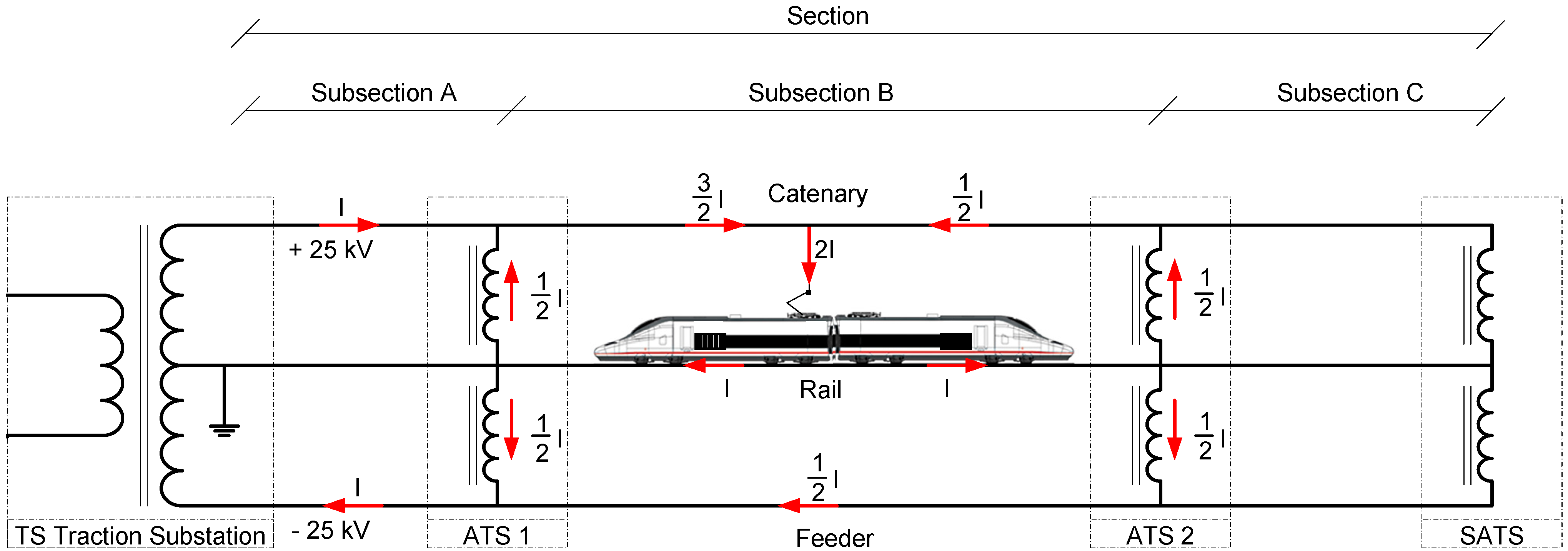
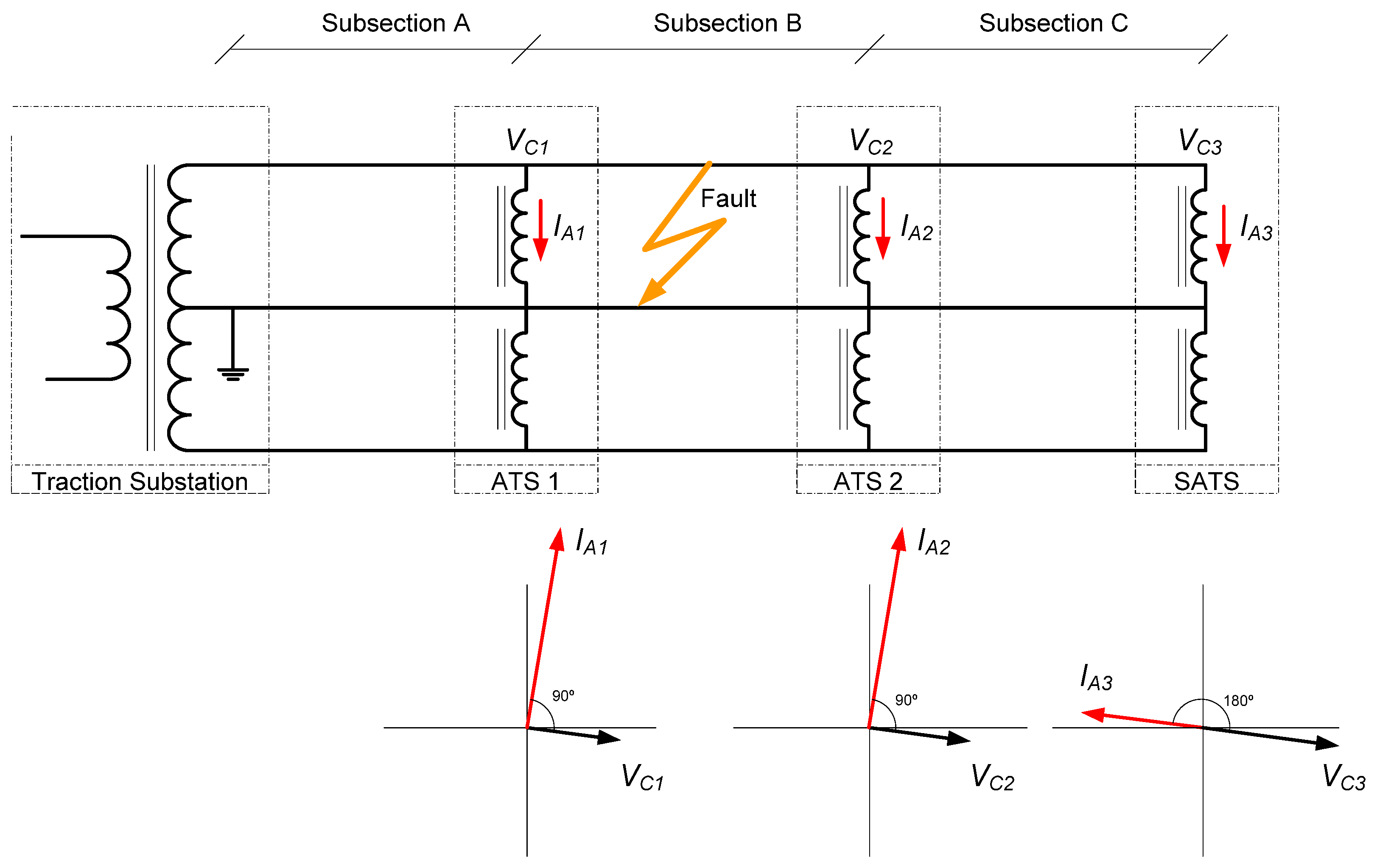
In these power systems, the complete traction line is supplied by several traction substations (TS). Each traction substation supplies two sections. Moreover, in each section, there are several subsections at regular intervals which are delimited by stations with power autotransformers (ATS). The autotransformer terminals are connected to the catenary and feeder, whereas its middle winding point is connected to the rail. At the end of each section another autotransformer station (SATS) is installed, where an autotransformer is connected in a similar way. In
Figure 1, a traction line section with three sub-sections is shown, as well as the theoretical current distribution.
Figure 1.
Simplified diagram of a 2 × 25 kV power system and current distribution in a section comprising three subsections.
Figure 1.
Simplified diagram of a 2 × 25 kV power system and current distribution in a section comprising three subsections.
In 2 × 25 kV power systems, the traction power demanded is delivered at 50 kV while it is used at 25 kV. This fact reduces the current needed to supply the power required by high-speed trains [
2]. In consequence, as this configuration presents lower losses and voltage drops along the line in comparison to 1 × 25 kV substation topologies, the length of the sections can be greater and the number of traction substations lower.
Another remarkable advantage of the 2 × 25 kV traction systems is the great reduction of electromagnetic interference on communication facilities and railway signalling circuits (signalling track circuits) as well as in nearby telecommunication lines [
3,
4].
Protection systems are essential to ensure the safe and efficient operation of any electrical installation [
5,
6]. Also, the proper management of these systems is an important factor to take into account in the profitability of these facilities [
7].
All electrical systems, especially railway traction systems, can have internal failures of their equipment and external faults caused by accidental events. Furthermore, in the traditional 1 × 25 kV power supply systems, most faults are caused by outdoor short circuits between the catenary and ground, while in the 2 × 25 kV power systems most of them are caused by outdoor short circuits between the catenary or the feeder to ground [
8,
9]. However, the detection and location of ground faults in the 2 × 25 kV lines are much more complex than in 1 × 25 kV lines, mainly because of the use of autotransformers [
10] in the ATS substations to which the catenary, feeder and rails are connected.
The complexity of the detection and location of ground faults in the 2 × 25 kV lines means that the identification of the subsection and the conductor where the ground fault has happened [
11,
12] is the main task of the protection systems in order to disconnect immediately the conductor with the ground fault in the corresponding subsection [
13]. This means only trains running in the subsection with the ground fault, in the case that the fault is in the catenary, will be disconnected from the power supply.
This paper describes a new method for identifying the subsection and the conductor (catenary or feeder) in which there is a ground fault in an easy and economical way. As the identification is done immediately, the subsection and conductor can be disconnected while keeping the rest of the power system in service. Another important advantage is that most of the elements that this method needs to be operative are already installed in any 2 × 25 kV power supply system, and consequently little new investment is required.
This new method has been validated through numerous computer simulations and experimental laboratory tests, obtaining excellent results. This paper first presents in
Section 2 an overview of the problem of ground fault location in 2 × 25 kV power systems and a brief description of the current methods. Then,
Section 3 details the principles of the proposed method, and
Section 4 presents an analysis of the simulations developed with MATLAB
® software.
Section 5 presents the results of experimental tests carried out in a laboratory set-up. Finally,
Section 6 concludes with the main contributions of the proposed new technique.
2. Ground Fault Location in 2 × 25 kV Power Systems: Description of the Problem
In traction power systems with ATS’s (2 × 25 kV), whose electrical scheme and current distribution are represented in
Figure 1, as well as in single-phase (1 × 25 kV) power systems, the main protection system is normally based on distance protection relays [
14]. These protection relays are usually installed at the traction substations and measure the impedance as the ratio between the voltage of the catenary and the difference of the catenary and feeder currents.
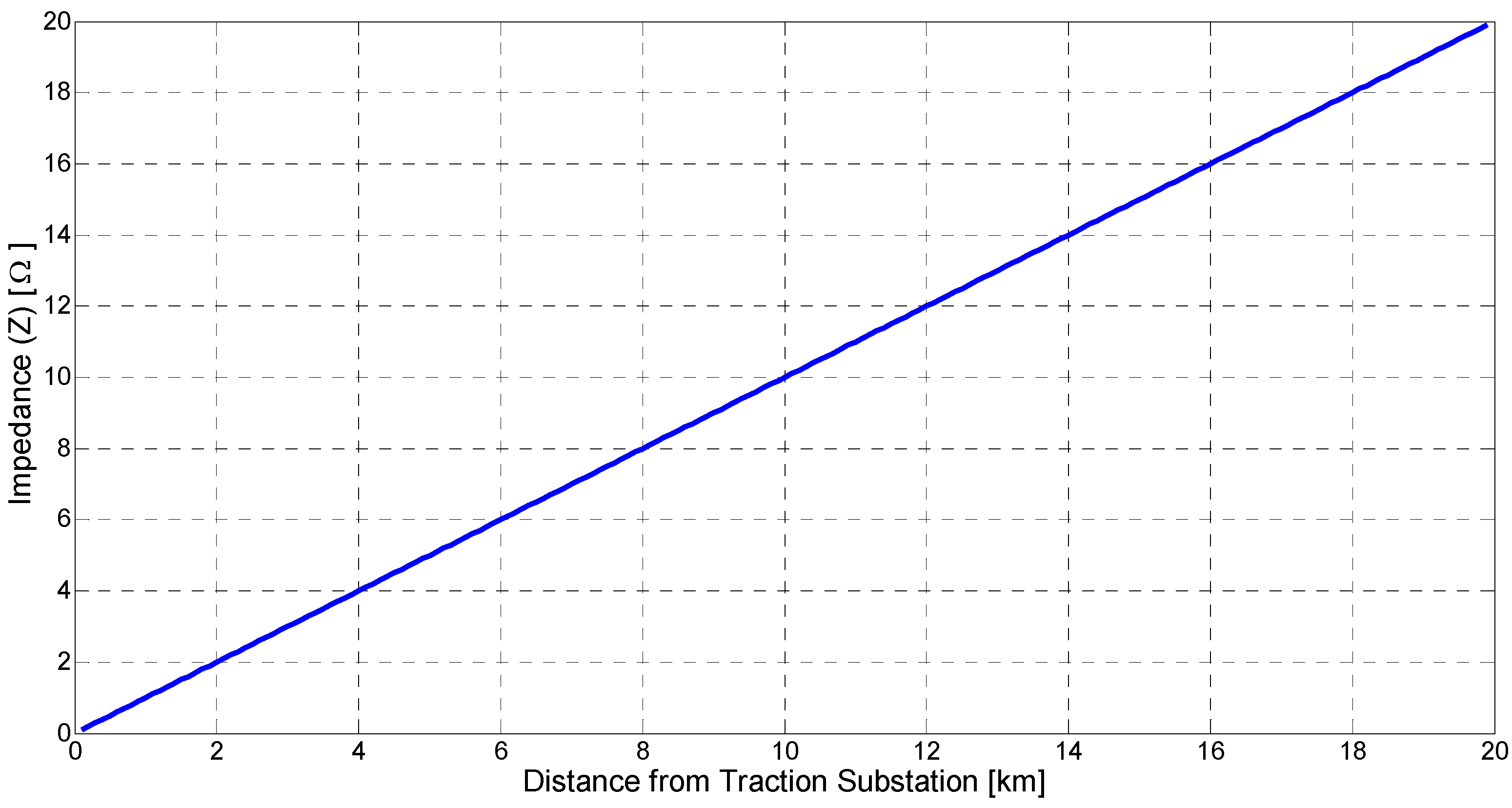
However, such traction power systems with ATSs (2 × 25 kV) do not make use of ground fault location based on the linear ratio between the impedance (Z) seen from the traction substation and the distance to the ground fault. This linear ratio, represented in
Figure 2, does, however, allow the distance protection relays to detect the ground fault and calculate the distance to the defect [
15,
16,
17] in one-conductor power systems (1 × 25 kV).
Figure 2.
Modulus of the fault impedance (Z) seen from the traction substation as a function of the distance in 1 × 25 kV traction power systems.
Figure 2.
Modulus of the fault impedance (Z) seen from the traction substation as a function of the distance in 1 × 25 kV traction power systems.
However, in traction power systems with ATSs (2 × 25 kV), the variation of the impedance value measured as a function of the distance to the ground fault is non-linear [
11,
16].
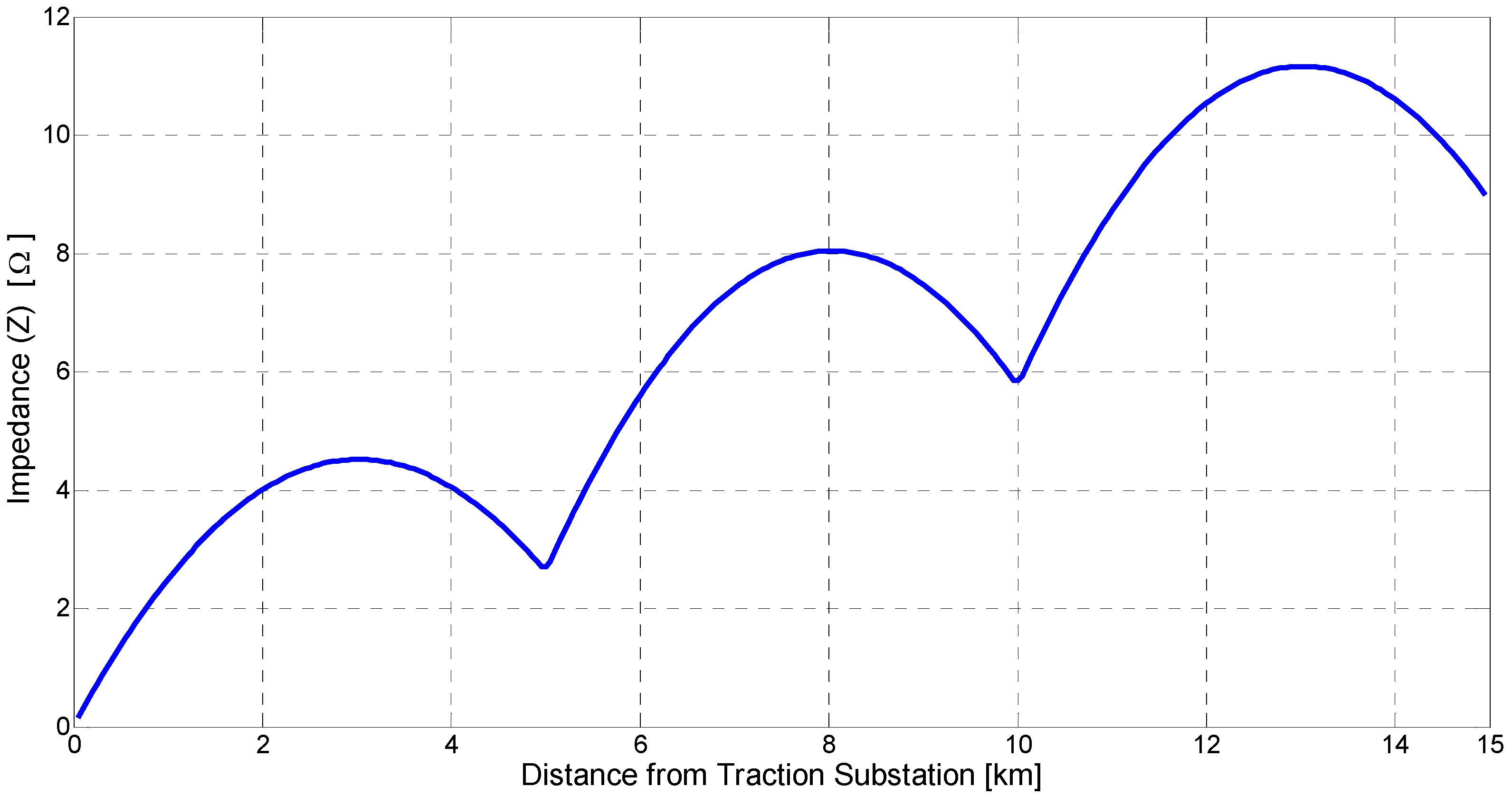
Figure 3 shows the real values of the fault impedance measured, where it can be seen that the ratio is non-linear in every subsection between two ATSs. The minimum values of the impedance measured correspond to the ATS’s emplacements.
Figure 3.
Modulus of the fault impedance seen from the traction substation in function of the distance in 2 × 25 kV traction power systems.
Figure 3.
Modulus of the fault impedance seen from the traction substation in function of the distance in 2 × 25 kV traction power systems.
Figure 3 reveals clearly that only measuring the modulus of the impedance to the ground fault in a subsection does not allow the location of the fault to be identified. Even when the modulus of the impedance is known, it is not possible to define in which subsection between two ATSs the ground fault has occurred, because the same value of measured impedance can be obtained from different subsections. As a result, it is standard practice at railway facilities to follow the protocol described in the following paragraphs.
When a ground fault happens, the distance protection relays register an impedance value lower than their settings values and a tripping command is released to the normally used double pole circuit-breakers in the substation, with a consequent interruption of the power supply in all subsections and ATS’s of the section with the defect.
After a pre-set time, the distance protection relays conduct automatic reclosing manoeuvres and again feed the subsections and ATSs, checking that the defect is not permanent. If the ground fault is still active, the distance protection relays switch off the circuit-breakers again and open the motor-driven disconnectors installed at the ATS’s substations. The next step is to switch on the circuit-breakers again. Now, as the catenary and feeder conductors are electrically isolated (the system operates as 1 × 25 kV), the distance protection relays will allow the conductor where the ground fault took place to be identified, as well as the relatively accurate identification of the subsection [
18].
To isolate the subsection with the ground fault, the information provided by the distance protection relay is used. As the circuits of the two conductors are now totally independent, the distance from the substation to the ground fault is obtained from the impedance measured by the distance protection relay. Once the subsection is isolated through its corresponding motor-driven disconnectors, the rest of the subsections without a ground fault are powered again. In the case of a lack of accuracy in the determination of the distance to the ground fault, a subsection which is closer to or farther away from the real distance to the fault may remain without power supply for an unacceptable time [
19].
To avoid this delay in the isolation of the true subsection with the ground fault, it is very useful to know, as soon as the ground fault has been detected, in which subsection between ATSs this has taken place and if it happened in the catenary or feeder conductor. The new system presented in this paper allows us to know just after the ground fault which subsection has the ground defect and if the fault is located between the catenary and rail or between the feeder and rail conductors. As this information is sent to the control centre immediately, automatic or manual decisions can be taken to restore the power supply to the subsections without any ground fault.
3. Principles of the New Ground Fault Subsection Identification Method
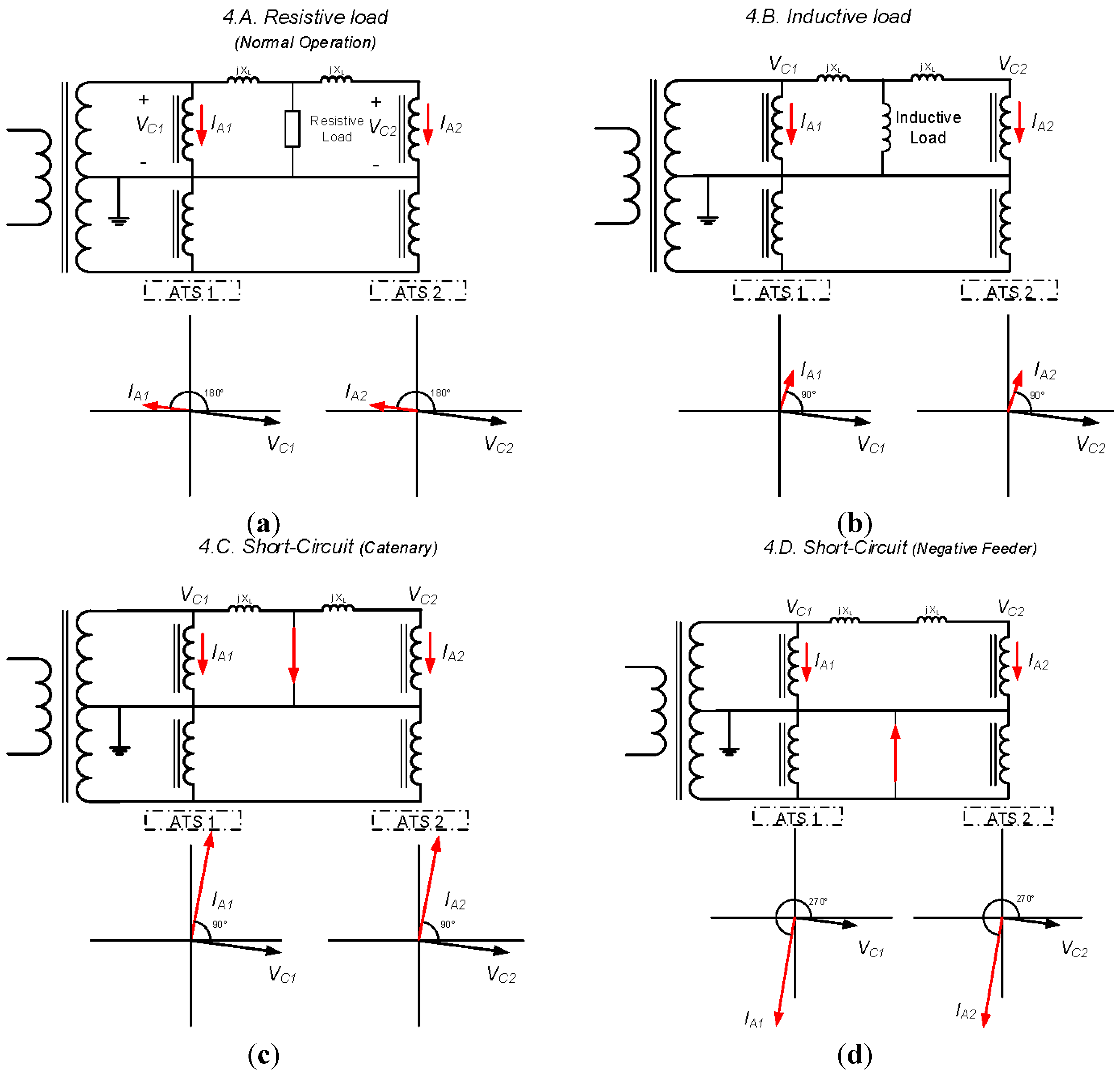
According to the theoretical current distribution of 2 × 25 kV power system (
Figure 1), the phase angle between voltage and current in the autotransformer is close to 180° in case of resistive load (
Figure 4a). In this case, the catenary inductance (X
L) can be neglected.
On the other hand, in case of an inductive load the phase angle between voltage and current in the autotransformer is close to 90°, as shown in the
Figure 4b.
The power factor of the high-speed trains is close to the unit; therefore, the current distribution under normal operation of a 2 × 25 kV power system is similar to the resistive load case shown in
Figure 4a.
The catenary short-circuit current is similar to the inductive load case, as the impedance seen from the autotransformer is the catenary inductance X
L. (
Figure 4c).
Finally in the
Figure 4d the feeder short-circuit case is represented, and it is symmetrical to the above case.
Figure 4.
2 × 25 kV theoretical currents distribution in case of resistive load (a); inductive load (b); short-circuit (catenary) (c); and short-circuit (negative feeder) (d).
Figure 4.
2 × 25 kV theoretical currents distribution in case of resistive load (a); inductive load (b); short-circuit (catenary) (c); and short-circuit (negative feeder) (d).
When there is a ground fault on a line between the catenary and rail or between the feeder and rail in a 2 × 25 kV traction power system, there is a substantial increase in the current circulating through the windings of the ATSs closest to the defect location. This current increase can be detected easily by measuring the currents in the windings of the ATSs. Furthermore, when the fault happens, the angles between the currents and voltages change in the ATSs closest to the fault location.
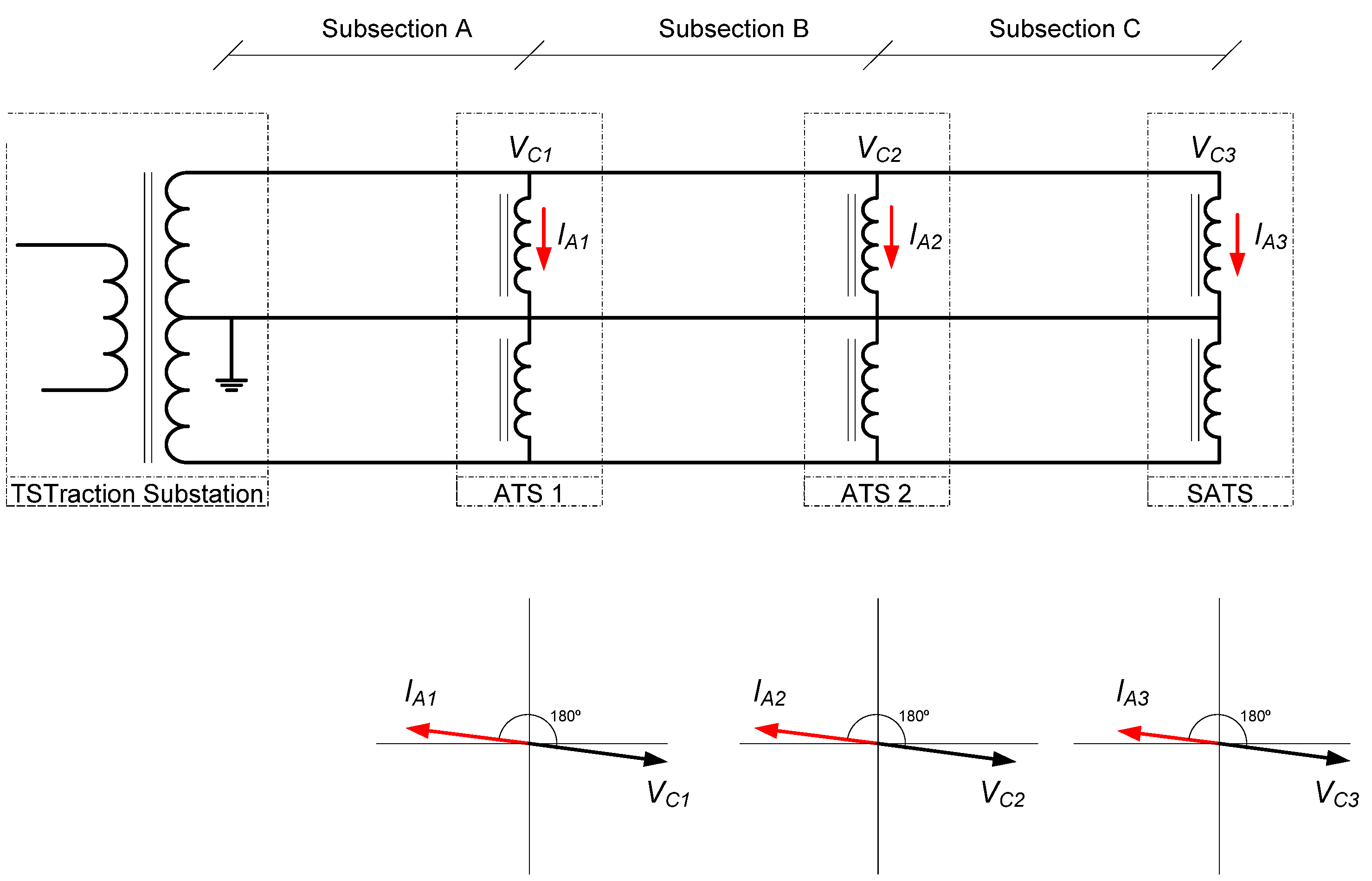
In normal operation, these angles between the currents and voltages in the autotransformers are close to 180°, as shown in
Figure 5. On the other hand, in the case of a ground fault, the phase angle between the voltage and current in the autotransformers will shift by 90°, as will be shown later.
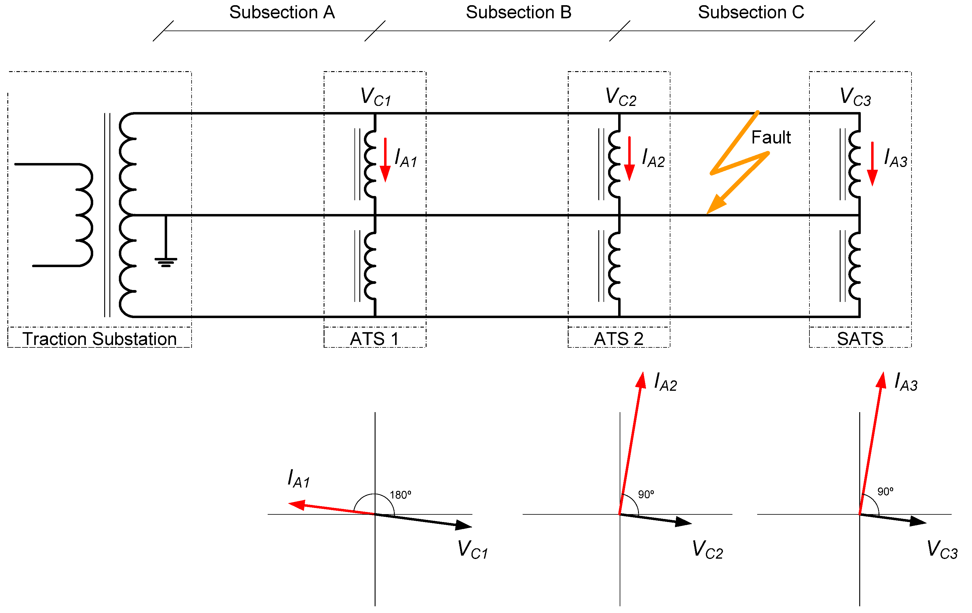
As an example, we can consider a ground fault in subsection C as shown in
Figure 6, where the modulus of the currents IA2 and IA3 increase their value by a great deal, whereas the current IA1 does not undergo any remarkable change in its value.
Figure 5.
2 × 25 kV power system currents (IA) and voltages (VC) distribution in normal operation.
Figure 5.
2 × 25 kV power system currents (IA) and voltages (VC) distribution in normal operation.
Figure 6.
2 × 25 kV power system currents (IA) and voltages (VC) distribution with a ground fault in the catenary in Subsection C.
Figure 6.
2 × 25 kV power system currents (IA) and voltages (VC) distribution with a ground fault in the catenary in Subsection C.
Furthermore, the angles between such currents I
A2 and I
A3 and the respective catenary to rail voltages V
C2 and V
C3 will change dramatically. In this case, as the fault is between the catenary and the rail in Subsection C, the angle between I
A2 and V
C2 changes in value from approximately 180° to 90° (see
Figure 5 and
Figure 6).
The angle between I
A3 and V
C3 is also reduced from close to 180° to near 90°. As indicated before, the angle between I
A1 and V
C1 remains stable with almost no variation, as can be seen in
Figure 6.
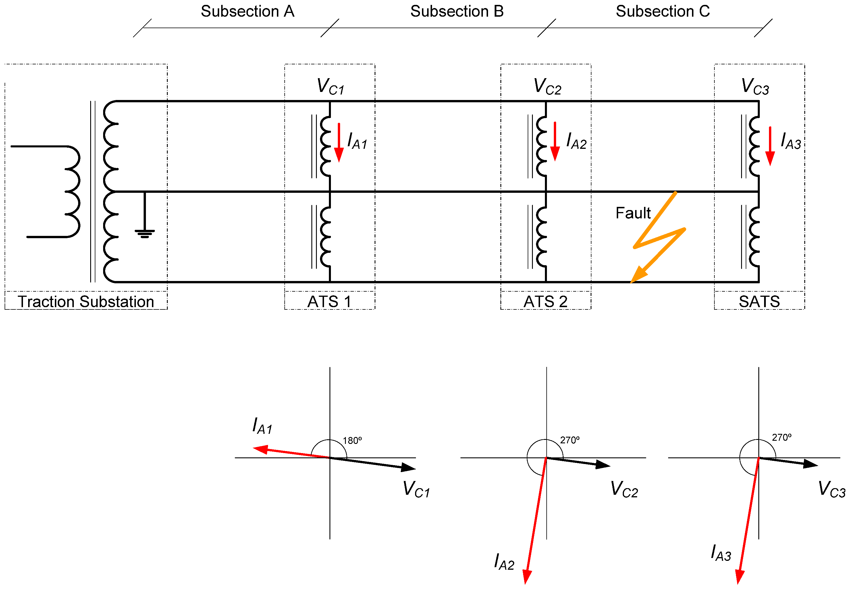
Now, if the ground fault happens in the same Subsection C but between the feeder and rail, the angle between I
A2 and V
C2 changes from 180° to 270° (see
Figure 5 and
Figure 7). There is also the same angle change between I
A3 and V
C3. Again, there is no significant change in the angle between I
A1 and V
C1.
If the ground fault happens in Subsection B, the current increase will affect only currents I
A1 and I
A2 and there will be no remarkable change in current I
A3. The angles between I
A1 and V
C1, and I
A2 and V
C2 respectively will change, but not the angle between I
A3 and V
C3. These phase angle changes will also be from 180° to 90° in the case of a fault between the catenary and rail (see
Figure 5 and
Figure 8), and from 180° to 270° if the fault is between the feeder and rail.
Figure 7.
2 × 25 kV power system current (IA) and voltage (VC) distribution with a ground fault in the feeder in subsection C.
Figure 7.
2 × 25 kV power system current (IA) and voltage (VC) distribution with a ground fault in the feeder in subsection C.
Figure 8.
2 × 25 kV power system currents (IA) and voltages (VC) distribution with a ground fault in the catenary in subsection B.
Figure 8.
2 × 25 kV power system currents (IA) and voltages (VC) distribution with a ground fault in the catenary in subsection B.
However, if there is a ground fault in Subsection A, only the current IA1 increases in value, while currents IA2 and IA3 remain stable with no significant changes in their values. Therefore, the change in the phase angle only affects the current IA1 and voltage VC1, but not the currents and voltages in the ATS2 and SATS. This variation in the phase angle between the current and voltage in the ATS1 installed at the end of the first subsection indicates that the ground fault is located in the first Subsection A.
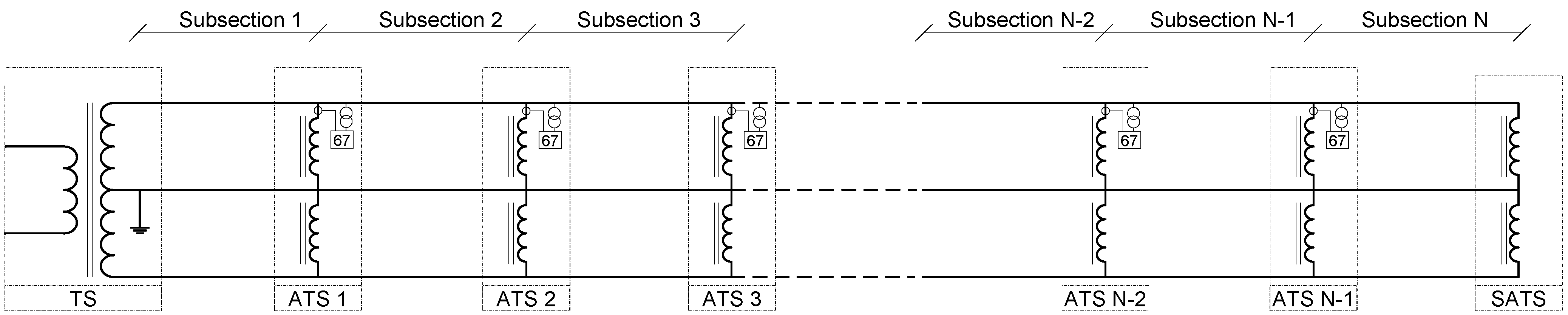
In fact, in facilities whose sections have more than two subsections, it is possible to avoid taking measurements at the station with ATS situated at the end of the last subsection (SATS). This is because when there is a current increase and a variation of the angle between the current and voltage only in the previous ATS (ATSN-1), the ground fault is located in the last subsection N.
Figure 9 represents a section formed by N subsections (with N > 2) with measuring devices for current and voltage in all stations with ATSs except in the last one (SATS).
Figure 9.
Section with N subsections supplied from the traction substation (TS) with N-1 measurement devices for current and voltage.
Figure 9.
Section with N subsections supplied from the traction substation (TS) with N-1 measurement devices for current and voltage.
The changes of the angle between the currents and voltages when there is a ground fault in the system represented in
Figure 9 are listed in
Table 1.
Table 1.
Angle variation between IA and VC as a function of the subsection with the ground fault.
Table 1.
Angle variation between IA and VC as a function of the subsection with the ground fault.
| Fault location | ATS1 | ATS2 | ATS3 | ATSN-3 | ATSN-2 | ATSN-1 |
|---|
| Fault at catenary in Subsection 1 | 90° | 180° | 180° | 180° | 180° | 180° |
| Fault at feeder in Subsection 1 | 270° | 180° | 180° | 180° | 180° | 180° |
| Fault at catenary in Subsection 2 | 90° | 90° | 180° | 180° | 180° | 180° |
| Fault at feeder in Subsection 2 | 270° | 270° | 180° | 180° | 180° | 180° |
| Fault at catenary in Subsection 3 | 180° | 90° | 90° | 180° | 180° | 180° |
| Fault at feeder in Subsection 3 | 180° | 270° | 270° | 180° | 180° | 180° |
| Fault at catenary in Subsection N-3 | 180° | 180° | 180° | 90° | 180° | 180° |
| Fault at feeder in Subsection N-3 | 180° | 180° | 180° | 270° | 180° | 180° |
| Fault at catenary in Subsection N-2 | 180° | 180° | 180° | 90° | 90° | 180° |
| Fault at feeder in Subsection N-2 | 180° | 180° | 180° | 270° | 270° | 180° |
| Fault at catenary in Subsection N-1 | 180° | 180° | 180° | 180° | 90° | 90° |
| Fault at feeder in Subsection N-1 | 180° | 180° | 180° | 180° | 270° | 270° |
| Fault at catenary in Subsection N | 180° | 180° | 180° | 180° | 180° | 90° |
| Fault at feeder in Subsection N | 180° | 180° | 180° | 180° | 180° | 270° |
If the variation of the phase angle between the current and voltage only takes place at the ATSN-1 installed between Subsections N and N-1, the ground fault is located in Subsection N. It is also observed that if the variation of such angle only happens in ATS1, the ground fault is in Subsection 1. Therefore, if variation of the angles between currents and voltages occurs in two ATS’s, the ground fault is in the subsection delimited by those ATS’s.
In the case that a section only has two subsections, it is also necessary to measure the currents and voltages at the installed end autotransformer SATS. If so, when there is only a variation in the angle between the current and voltage in ATS1, the ground fault is in the first subsection, and if the fault occurs in the second subsection, the angle variation happens at both ATS1 and SATS.
If the angle is measured between the incoming current from the feeder in the winding of each ATS and catenary voltage VC, in the case of a fault between the catenary and rail, this angle will be 270°, whereas if the fault is located between the feeder and rail, this angle will now be 90°. This angle situation is exactly the opposite when the incoming current in the winding of each ATS from the catenary is measured.
4. Experimental Simulations
In order to check the validity of the fundamentals of the proposed new method, numerous simulations were carried out using MATLAB
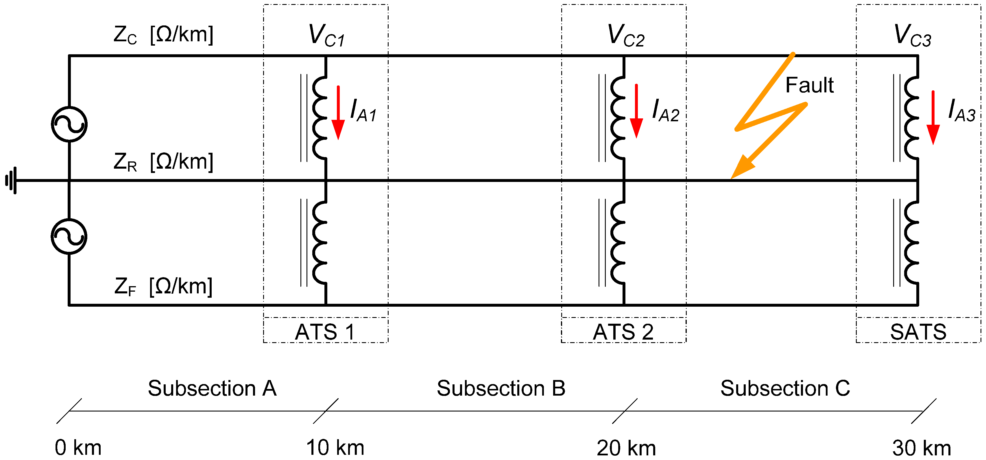
® software. For this purpose, the circuit shown in
Figure 10 was programmed using the modified nodal circuit analysis method [
20]. The experimental circuit is supplied from one end with two 25 kV AC sources with reverse polarity in each one. This circuit has three parts, A, B and C, each with a length of 10 km
Figure 10.
Simulated power supply system with two conductors and return grounded wire 2 × 25 kV.
Figure 10.
Simulated power supply system with two conductors and return grounded wire 2 × 25 kV.
To obtain the self-impedance values per length unit of the catenary Z
C, the feeder Z
F and rail connected to ground Z
R, as well as the mutual impedances between the conductors Z
CR, Z
FR and Z
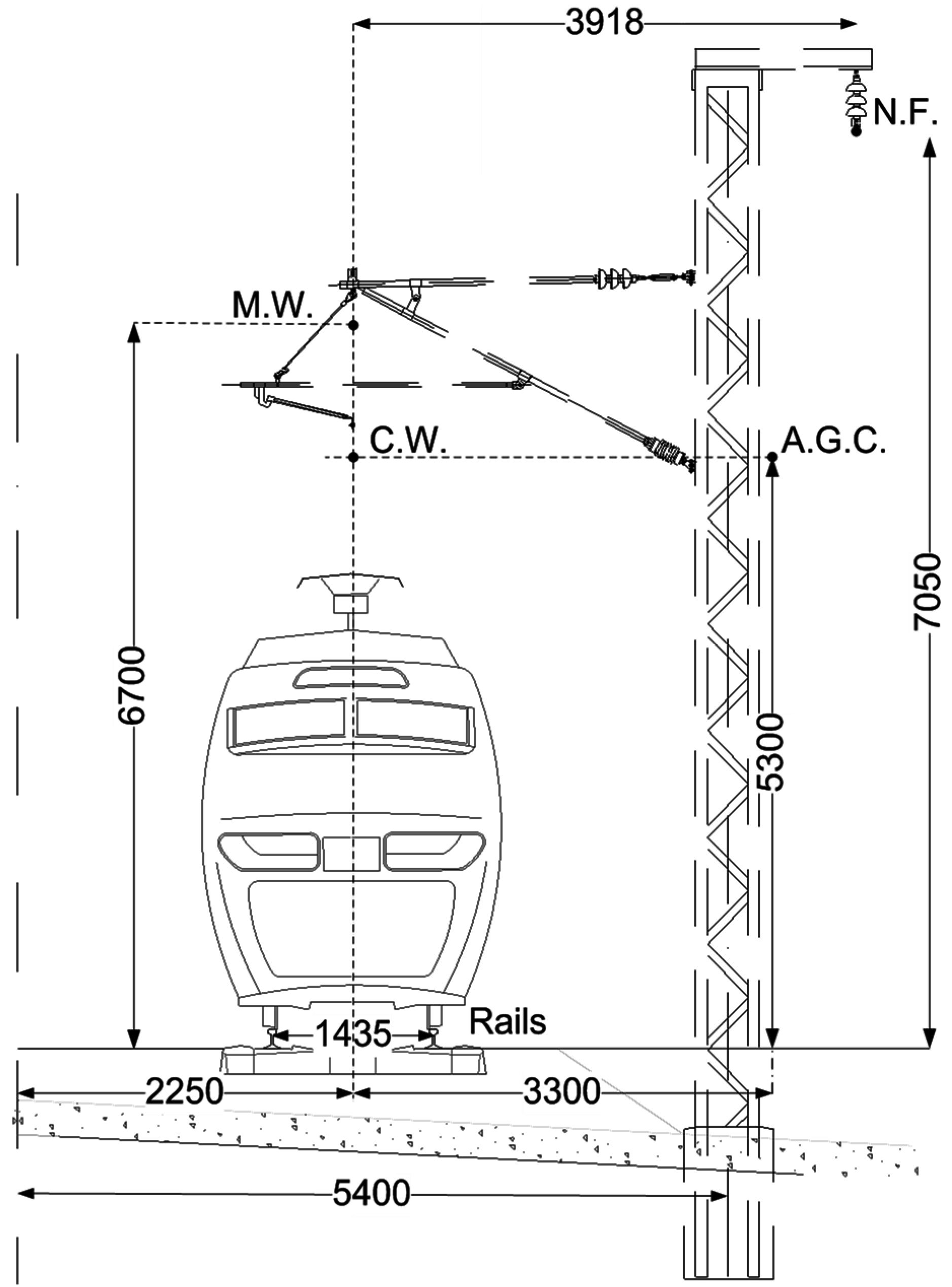
CF, a new ATP software model was developed, including the geometry of the railway with five conductors. This ATP software model is shown in
Figure 11 and uses resistance values per length unit as listed in
Table 2. With such data incorporated into the ATP model, the impedance values obtained are given in
Table 3.
Table 2.
Resistance values of the railway per length unit.
Table 2.
Resistance values of the railway per length unit.
| Conductor | Resistance Ω/km |
|---|
| Contact wire (C.W.) | 0.115 |
| Messenger wire (M.W.) | 0.172 |
| Negative feeder (N.F.) | 0.062 |
| Aerial ground conductor (A.G.C) | 0.119 |
| Rails | 0.026 |
Table 3.
Self and mutual impedances values of the railway conductors.
Table 3.
Self and mutual impedances values of the railway conductors.
| Conductor | Impedance Ω/km |
| Catenary | ZC | 0.1197 + j0.6224 |
| Feeder | ZF | 0.1114 + j0.7389 |
| Rail | ZR | 0.0637 + j0.5209 |
| Conductors | Impedance Ω/km |
| Catenary-Feeder | ZCF | 0.0480 + j0.3401 |
| Catenary-Rail | ZCR | 0.0491 + j0.3222 |
| Feeder-Rail | ZFR | 0.0488 + j0.2988 |
Figure 11.
Railway geometry used for the model developed in ATP software (distances in mm).
Figure 11.
Railway geometry used for the model developed in ATP software (distances in mm).
These data obtained from the ATP railway model were implemented in the circuit shown in
Figure 10. Employing this circuit, different MATLAB
® simulations were developed, performing short-circuits between the catenary and rail, and between the feeder and rail. These short-circuits were simulated at all the points along the three Subsections A, B and C of the 30 km section. The phase angles between the currents I
A1-I
A2-I
A3 and the voltages V
C1-V
C2-V
C3 in the autotransformers ATS1, ATS2 and SATS, as a function of the distance from the traction substation where the fault has happened between the catenary and rail, are represented in
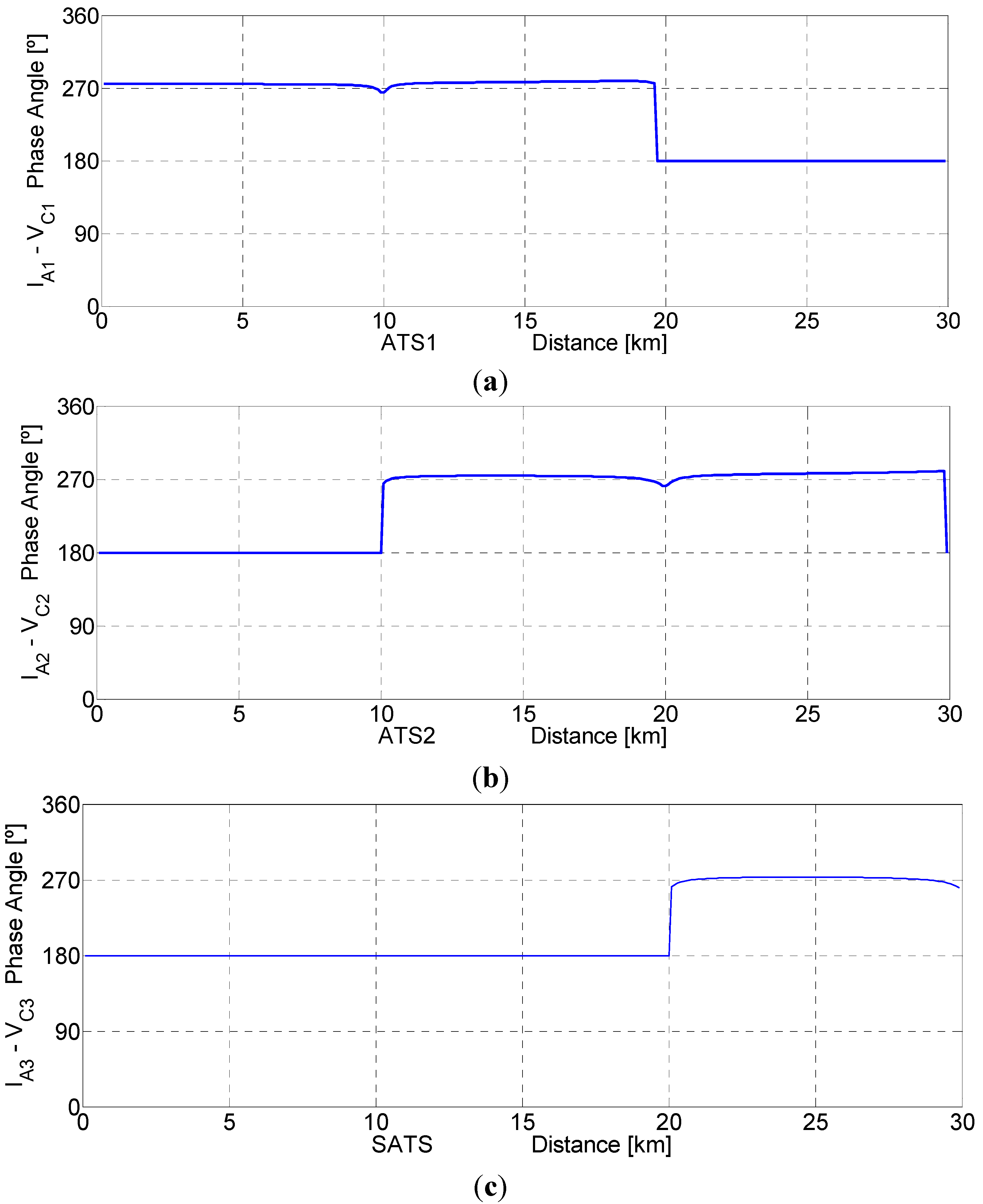
Figure 12. The axes used in
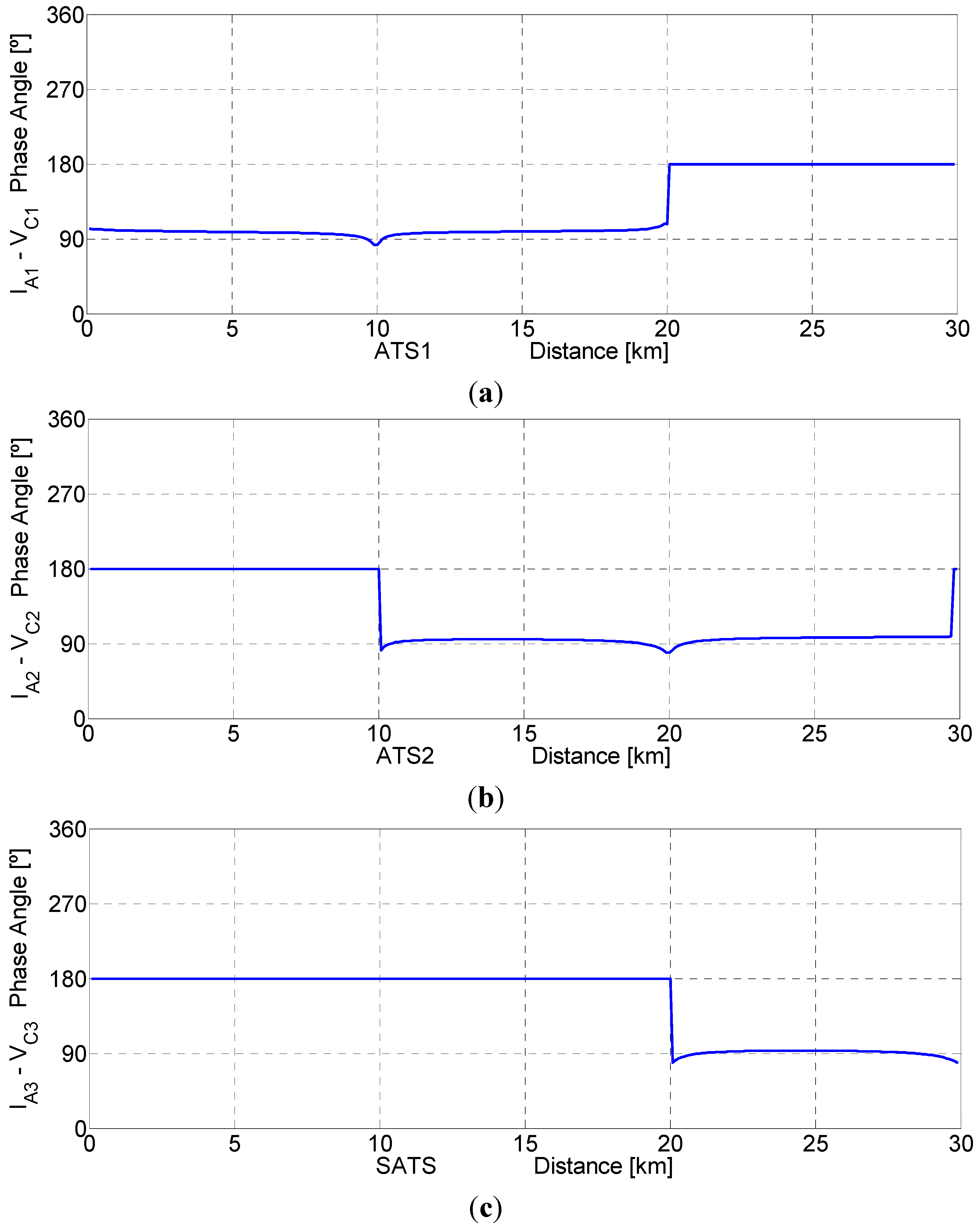
Figure 12 are scaled from 0 to 30 km and from 0° to 360°. It can be observed that if the fault happens in Subsection A along the first 10 km, the angle between the current I
A1 and voltage V
C1 in the ATS1 is about 90°. However, such angles at ATS2 and SATS are 180°. Likewise, if the fault is in Subsection B (between 10 and 20 km) the phase angles between the current I
A1 and the voltage V
C1, and between the current I
A2 and the voltage V
C2, will be about 90° at both ATS1 and ATS2, while at SATS this angle is close to 180°. It can also be seen that if the fault is in Subsection C (between 20 and 30 km), the angle is about 90° at ATS2 and SATS but 180° at ATS1.
Figure 12.
Phase angles between IA and VC at different ATSs as a function of the distance to the fault from the substation. Fault considered between catenary and rail. ATS1 (a); ATS2 (b) and SATS (c).
Figure 12.
Phase angles between IA and VC at different ATSs as a function of the distance to the fault from the substation. Fault considered between catenary and rail. ATS1 (a); ATS2 (b) and SATS (c).
In the case that the fault happens between the feeder and rail, as expected in the theoretical research, the results obtained are similar when the fault takes place between the catenary and rail, except that now the angles between the currents I
A1-I
A2-I
A3 and the voltages V
C1-V
C2-V
C3 are 270° instead of 90°.
Figure 13 shows how the variations of these phase angles as a function of the distance to the fault from the substation follow the same pattern as in the case of a fault between the catenary and rail, but now with values close to 270°.
Figure 13.
Phase angles between IA and VC at different ATS’s as a function of the distance to the fault from the substation. Fault considered between feeder and rail. ATS1 (a); ATS2 (b) and SATS (c).
Figure 13.
Phase angles between IA and VC at different ATS’s as a function of the distance to the fault from the substation. Fault considered between feeder and rail. ATS1 (a); ATS2 (b) and SATS (c).
The results obtained from all the simulations developed confirm the theoretical values listed in
Table 1, and therefore the identification of the conductor and subsection with the ground fault is totally successful.
5. Experimental Laboratory Tests
Besides the computer simulations, multiple tests were performed in the laboratory with the aim of getting, in a practical way, results that allow the identification of the conductor and subsection with the ground fault. These tests followed the circuit configuration indicated in
Figure 14.
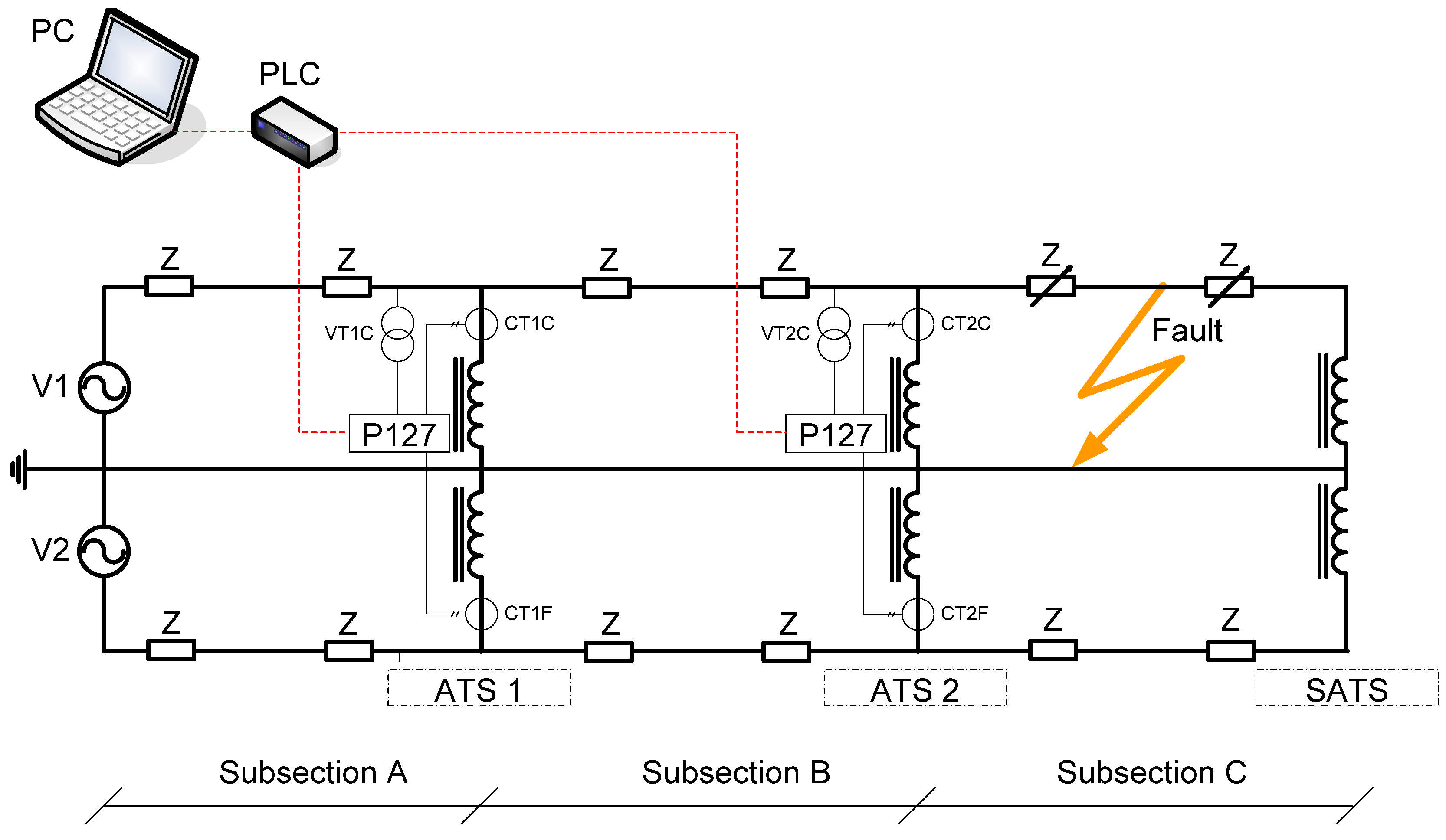
Figure 14.
2 × 25 kV experimental set-up of simplified circuit (one section with three subsections).
Figure 14.
2 × 25 kV experimental set-up of simplified circuit (one section with three subsections).
Figure 15.
Experimental set-up circuit to simulate ground faults in laboratory.
Figure 15.
Experimental set-up circuit to simulate ground faults in laboratory.
The distributed impedance of the catenary and feeder was achieved using inductive impedances Z and two voltage sources, V1 and V2, supplying 100 V.
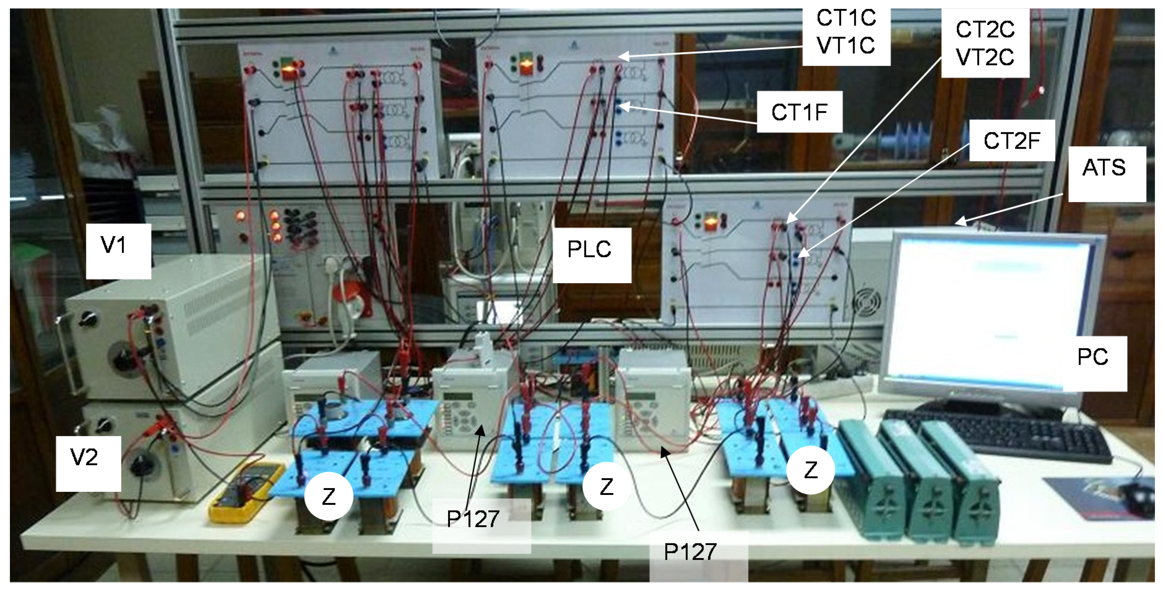
The section was divided into three Subsections A, B and C through ATS’s. At the intermediate ATS’s only (ATS1 and ATS2), measurement and control devices were installed: voltage transformers (VT1C and VT2C) were connected between the catenary and the 0 V conductor, current transformers (CT1C and CT2C) were installed in the winding of the ATSs connected to the catenary, current transformers (CT1F and CT2F) were installed in the winding of the ATSs connected to the feeder, and directional overcurrent relays (P127) were included to register the current and voltage measurements.
Figure 15 shows the experimental set-up.
The directional overcurrent relays (P127) are MiCom P127 type with analogue inputs for the current and voltage signals obtained from the VT’s and CT’s. Current transformers CT1C and CT2C measure the currents IA1 and IA2 that enter from the positive terminals in ATS1 and ATS2. Voltage transformers VT1C and VT2C measure the voltage VC at the connection points of each ATS to the catenary. Current transformers CT1F and CT2F measure the currents that enter the ATS1 and ATS2 from the connection point to the feeder. Such currents and voltages are driven to the protection relay P127. In the protection relay P127, at ATS1, the current input assigned to phase A is connected to the current transformer CT1C, the current input assigned to phase B is not used, and the current input assigned to phase C is connected to current transformer CT1F. Voltage inputs for phases A and C are connected to the 0 V conductor, whereas the voltage input for phase B is connected to the voltage transformer VT1C. The same connections are used for ATS2 measurements.
The protection relay P127 was set to release a tripping command when the currents measured had values over the previous adjusted setting and when the angle between the voltage VC and the currents measured by CTCs or CTFs is approximately 90°. To guarantee the correct operation of the directional overcurrent relays (P127), a range in the angle setting is required. After analysis of the experimental results, we find that an angle setting range from 60° to 120° (90° ± 30°) is appropriate. This angle range should be adapted for a particular 2 × 25 kV supply system.
When the tripping command given by the protection relay P127 is in response to the currents provided by CT1C or CT2C, the output free of potential contact RLP1 or RLP2 is activated at the corresponding P127 protection relay. This situation corresponds to a fault between the catenary and rail with high current circulating from the catenary and with an angle of about 90° between the corresponding current and voltage.
Another option for tripping commands given by the protection relay P127 is in response to the currents provided by CT1F or CT2F. Now the output free of potential contact RLN1 or RLN2 is activated. This situation corresponds to a fault between the feeder and rail with high current circulating from the feeder and an angle between such currents and the voltage VC also close to 90°.
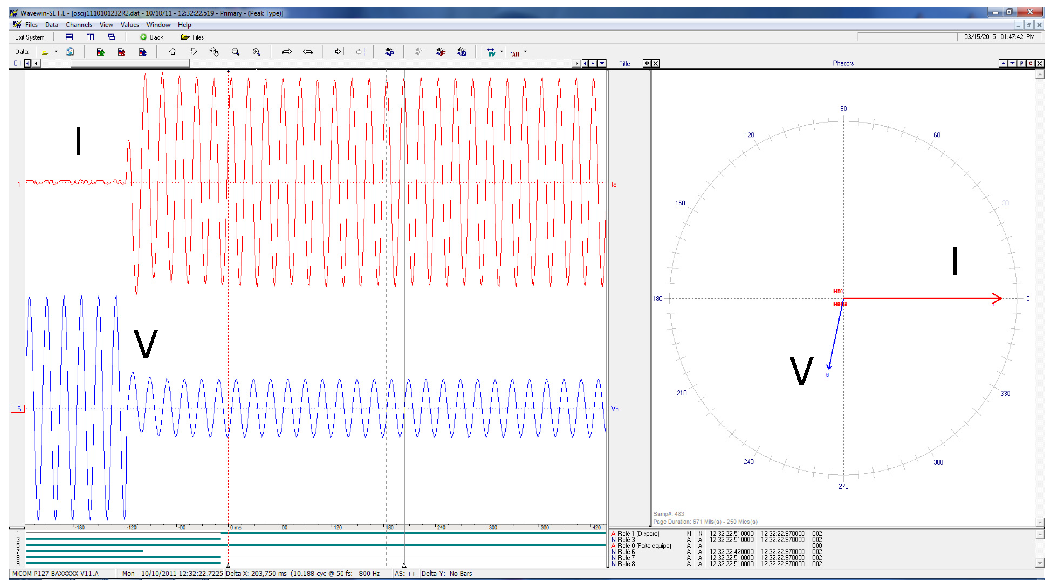
Figure 16 shows, as an example of one of the tests performed, a disturbance record provided by the protection relay P127 when a fault has happened between the catenary and the 0 V rail conductors. The tripping command is sent through the output contact RLP as the angle between the incoming current from the catenary and the voltage is close to 90°.
If the fault happens in the first Subsection A, the tripping command will be delivered by output contacts RLP1 or RLN1 only in the first protection relay. If the fault is located in Subsection B, protection relays 1 and 2 will activate their corresponding output contacts for tripping. Finally, if the fault is in Subsection C, only the output contacts for tripping in relay 2 will be activated. These options are listed in
Table 4, where SA indicates any output that has been activated. Any output contact which is not activated is represented in
Table 4 as NO.
Figure 16.
Disturbance record from the protection relay P127. Current and voltage in ATS during a fault between catenary and 0 V conductor.
Figure 16.
Disturbance record from the protection relay P127. Current and voltage in ATS during a fault between catenary and 0 V conductor.
Table 4.
Activation of the output contacts of the protection relays as a function of the subsection and conductor with fault.
Table 4.
Activation of the output contacts of the protection relays as a function of the subsection and conductor with fault.
| Fault location | RLP1 | RLN1 | RLP2 | RLN2 |
|---|
| Fault at catenary in Subsection A | SA | NO | NO | NO |
| Fault at feeder in Subsection A | NO | SA | NO | NO |
| Fault at catenary in Subsection B | SA | NO | SA | NO |
| Fault at feeder in Subsection B | NO | SA | NO | SA |
| Fault at catenary in Subsection C | NO | NO | SA | NO |
| Fault at feeder in Subsection C | NO | NO | NO | SA |
Both RLP and PLN output contacts of every directional protection relay are connected to a programmable logic controller (PLC). This PLC evaluates all RLP and RLN inputs and, following the protocol described in
Table 4, a signalizing message specifying which conductor and subsection have suffered the fault is sent to a PC for visualization.
6. Conclusions
A new method for identification of the subsection and conductor with a ground fault has been presented in this paper. It is suitable for 2 × 25 kV railway supply networks when the use of autotransformers makes location of the ground fault a very complex task.
This new method is based on comparison of the phase angle between currents and voltages in the catenary of each autotransformer. Depending on the value of these phase angles, it is possible to identify the subsection and the conductor with the ground fault. In other words, it is possible to know between which autotransformers the fault has occurred and if the ground fault involves the catenary or the feeder conductor.
Numerous experimental laboratory tests and MATLAB® simulations were performed, with different ground faults in all the subsections of a 2 × 25 kV model.
The results show that the phase angles between currents and voltages change in the adjacent autotransformers when a ground fault takes place between them. In the case of a ground fault on the catenary, the angle changes to 90°, and in the case of ground fault in the feeder, the angle changes to 270°. On the other hand, in the remaining autotransformers the angle remains close to 180°. In both computer simulations and laboratory tests, the results were totally satisfactory, verifying the successful operation of the method.
This new identification method, compared to traditional ground fault location methods, has the following advantages:
It can distinguish the subsection directly after the ground fault occurs.
-
No additional tests are required to locate the subsection with the ground defect.
The feeder and the subsection affected by the ground fault can be disconnected in a short time, keeping the rest of the power system in service.
The method is based on phase comparison, so a standard directional overcurrent relay can be used, which represents an economic advantage.


