
Finite Time Analysis of a Tri-Generation Cycle

1
School of Mechanical and Systems Engineering, Newcastle University, Newcastle upon Tyne NE1 7RU, UK
2
Faculty of Engineering and Environment, Northumbria University, Newcastle upon Tyne NE1 8ST, UK
3
School of Marine Sciences and Technology, Newcastle University International Singapore (NUIS), Singapore 599493
*
Author to whom correspondence should be addressed.
Energies 2015, 8(6), 6215-6229; https://doi.org/10.3390/en8066215
Submission received: 28 February 2015
/
Revised: 13 June 2015
/
Accepted: 15 June 2015
/
Published: 23 June 2015
(This article belongs to the Special Issue Tri-Generation Cycles, Combined Heat, Power and Cooling (CHPC))
Abstract
:A review of the literature indicates that current tri-generation cycles show low thermal performance, even when optimised for maximum useful output. This paper presents a Finite Time analysis of a tri-generation cycle that is based upon coupled power and refrigeration Carnot cycles. The analysis applies equally well to Stirling cycles or any cycle that exhibits isothermal heat transfer with the environment and is internally reversible. It is shown that it is possible to obtain a significantly higher energy utilisation factor with this type of cycle by considering the energy transferred during the isothermal compression and expansion processes as useful products thus making the energy utilisation larger than the enthalpy drop of the working fluid of the power cycle. The cycle is shown to have the highest energy utilisation factor when energy is supplied from a low temperature heat source and in this case the output is biased towards heating and cooling.
1. Introduction
Combined cooling, heat, and power (CCHP) systems—also called tri-generation systems—are the combination of cogeneration plants and refrigeration systems (often absorption chillers) that offer a solution for generating electrical power, space or water heating, air conditioning and/or refrigeration. This is very useful for sites such as hospitals, supermarkets, airports that have a requirement for this range of applications. Other arrangements of systems have included desalination equipment that can make use of low grade waste thermal energy at periods of low demand elsewhere to produce a saleable product. The use of absorption refrigeration equipment eliminates the use of hydrochlorofluorocarbons/chlorofluorocarbons (HCFC/CFC) refrigerants and the overall combined cycle reduces overall emissions with high levels of fuel efficiency. Examples of this technology include the Jenbacher plant that serves a shopping mall and multi-screen cinema in the town of Celje, near Maribor (Slovenia) which was commissioned by TUS, Slovenia’s second-largest grocery chain, and has been operating since February 2003. The refrigeration output of the system is used all year round to cool a nearby refrigerated warehouse and during the summer months, the air-conditioning plant of the shopping mall and cinema is also supplied with cooling. In winter, the plant also provides heat for the entire complex. The electricity generated is sold directly to the local electricity utility company. The system can also operate in island mode and provide power to the complex in the event of a grid failure.
The energy utilisation factors (EUF) of contemporary tri-generation cycles are very low considering that similar or higher values were predicted by Horlock [1] for CHP cycles. This may be due to the accounting method used in the analysis in defining useful output or it may be due to losses within the tri-generation cycle. In another paper Horlock [2] considered the maximum theoretical output from a CHP plant when both work and heat are considered to be prime products. He showed that there was no maximum (network plus useful heat rejection) for flow between states 1 and 2 in the presence of a sink at T0. In examining different processes between states 1 and 2 Horlock showed that combinations of isentropic and isothermal processes, including an isothermal expansion at the sink temperature T0 leads to an EUF larger than that achievable from the enthalpy drop (h1–h2) between the initial and final states. This is due to the heat pumped from the sink being utilized. If this information is applied to tri-generation cycles it implies that such cycles should be composed of isentropic and isothermal processes to obtain maximum energy utilisation. A suitable candidate cycle is the Carnot cycle or any cycles that have isothermal heat addition and rejection and are internally reversible such as the Stirling cycle. The following work focuses on a tri-generation cycle composed of combined Carnot cycles that have been optimised for maximum power output. It is well known that the Carnot cycle represents the upper bound for work output from a given energy source but as shown by Curzon and Ahlborn [3] the power output is zero due to the infinitely long times required by the isothermal processes to remain at constant temperature. Finite Time Thermodynamics (FTT) was developed as a result of their work to examine the maximum power that could be produced by an irreversible Carnot cycle and other energy transformation processes [4,5,6,7,8,9,10,11,12,13,14,15,16]. Previous studies [15,16] have compared the efficiency values of this approach with that of actual plant and have shown good agreement such that FTT is considered to be a reasonable yard stick by which to assess the performance of practical cycles. This has been extended in this paper to provide an approximate value of the EUF that it is expected could be achieved from a practical tri-generation cycle.
2. Literature Review
Combined thermodynamic cycles have been proposed for many years to recover waste heat, thus improving the overall energy conversion efficiency of the cycle and reducing carbon emissions. Initially these took the form of Combined Heat and Power cycles (CHP) in which the energy in the exhaust gases of the power cycle was recovered to energise a steam turbine and/or provide energy for district heating and hot water production [1,2]. For some time now combined power and cooling cycles (CCP) have been proposed using multi-component fluids in order to reduce heat transfer related irreversibilities [17,18,19] and have shown typically a 10%–20% improvement in thermal efficiency compared to a Rankine cycle alone. More recently tri-generation cycles that produce combined heat, power and refrigeration have been proposed for specific situations. The food manufacturing and retail industries that have a need for heating, electrical power and refrigeration have been considered by Tassou et al. [20]. Similar studies have been performed in several other authors [21,22,23].
In the retail applications heating systems typically employ low pressure hot water, high pressure hot water or steam, vapour compression refrigeration systems and an electrical power supply derived from the electricity distribution system. The overall utilisation efficiency of these processes is low, because of the relatively low electricity generation efficiency of some power stations and associated distribution losses. Tri-generation is seen as a way of increasing the energy utilisation efficiency of food manufacturing and retail facilities by integrating the various waste and demand energy streams into an integrated system. Such systems can reduce CO2 emissions by 10% to 50% or even more depending on the conditions. The best solutions correspond to the use of non-fossil fuel and total energy systems. The results of studies [22,23] indicated the economic viability of these systems (subject to the price of natural gas and grid electricity) with payback periods of less than 4.0 years. A bio fuel based tri-generation system is seen as one of the very few technologies capable of contributing to reducing the rate of atmospheric CO2 concentration.
Optimisation studies [24,25,26] of tri-generation systems have been conducted by several authors. These are combinations of conventional cycles with the refrigeration effect being produced by compression refrigeration units or waste heat driven absorption refrigerators. Energy utilisation factor (EUF) values vary between 47% and 70% which indicates the extent of the internal irreversibilities of the cycle components. These values are relatively low considering that Horlock [1] was quoting values in excess of this for Rankine cycle based CHP cycles. The key to this, as indicated by Horlock, must lie in management of the energy transfer processes within the cycle and between the cycle and the environment. Horlock showed in this paper that the best exergetic efficiency was obtained when the energy extracted from the “conceptual environment” was utilised effectively. This can be achieved by isothermal processes of heat addition and rejection and if these are part of a thermodynamic cycle this must be internally fully reversible. A number of cycles can meet these requirements including the Carnot and Stirling cycles, which can deliver Carnot efficiency and can also operate in reverse as a refrigerator. A combined cycle of coupled power and refrigeration elements based on these theoretical cycles has the potential of operating in a tri-generation mode making use of the energy of the refrigeration effect to augment the network output.
Finite time thermodynamics was developed from the concept of internally reversible and externally irreversible Carnot cycles. Based upon this premise a new methodology of thermodynamic analysis was developed that has become known as the Novikov-Curzon-Ahlborn process [14]. Several methods, of varying degrees of sophistication for studying the performance of endoreversible heat engines have been suggested [14,15,16,17,18,19,20] that have identified the operational bounds of thermodynamic processes. Initially this work was concerned with single stage power cycles but cooling cycles have been represented by Rozonoer et al. [9], and Kaushik et al. [10]. Combined operating in a sequential mode has also been considered [11,12,13,14] as have combined power and refrigeration cycles [15] with emphasis on absorption refrigeration systems.
3. Analysis
The following analysis is based on a Carnot cycle but it is applicable to a Stirling cycle and any cycle that has isothermal energy exchange with the environment and is internally fully reversible. The Carnot cycle is a theoretical concept only that illustrates the efficiency bounds of thermodynamic cycles but the Stirling cycle is a well-established external heating cycle that lends itself to the utilisation of waste heat, is reversible and is relatively easy to connect to heat sources and heat sinks. This cycle has been investigated extensively because of its potentially high thermal efficiency, low emissions and tolerance to fuel type. As a prime mover it has been fitted to buses in California but its low power output per unit volume makes it better suited for stationary applications. A T-S diagram of a Carnot cycle is shown in Figure 1.
Figure 1.
T-S diagram of a Carnot Cycle.
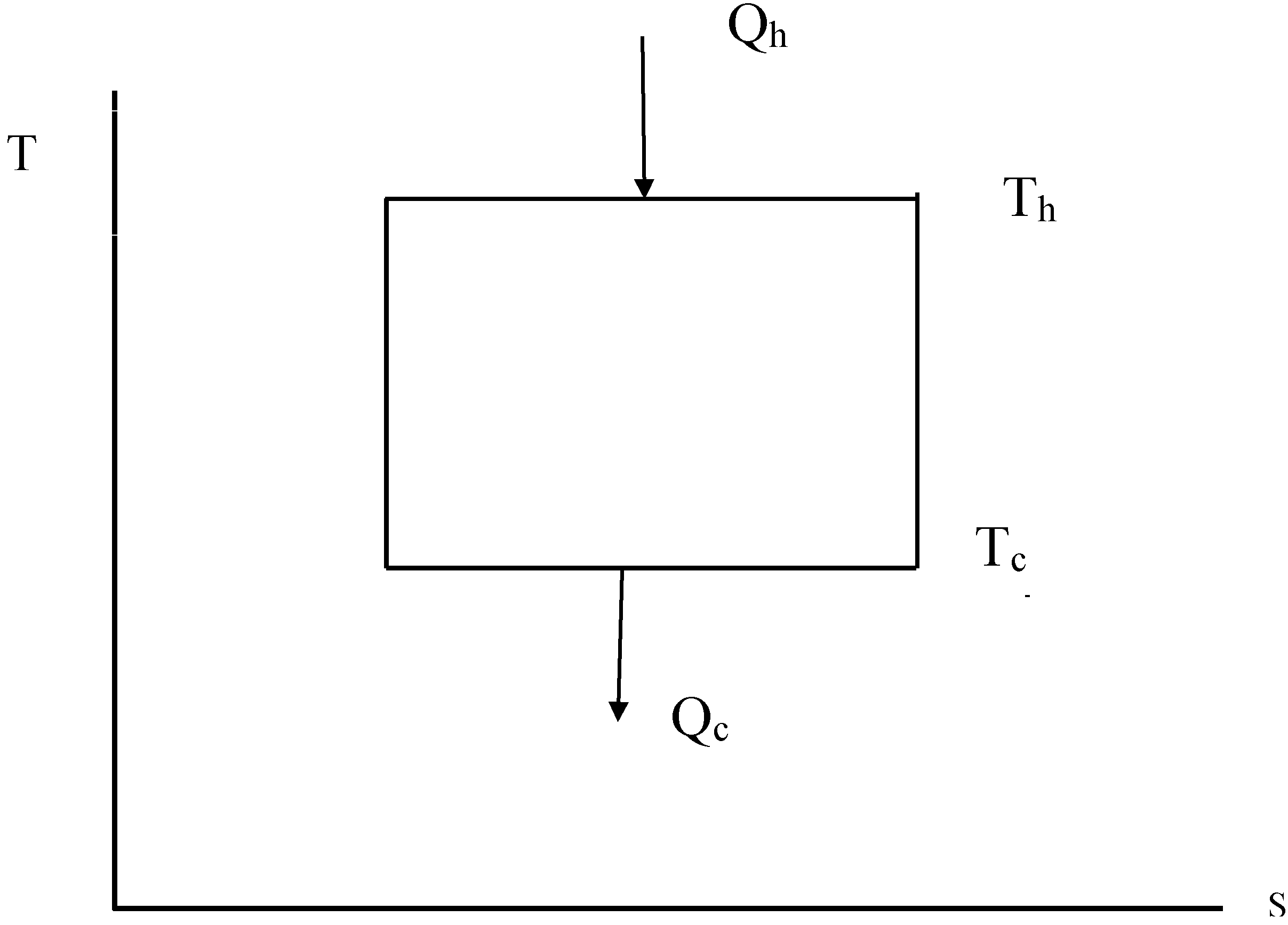
The energy transfer in the isothermal processes for a cycle using an ideal gas as the working fluid can be expressed as:
which results in the well-known Carnot efficiency:
where Tc and Th represent the temperatures of the cold and hot isothermal processes, respectively.
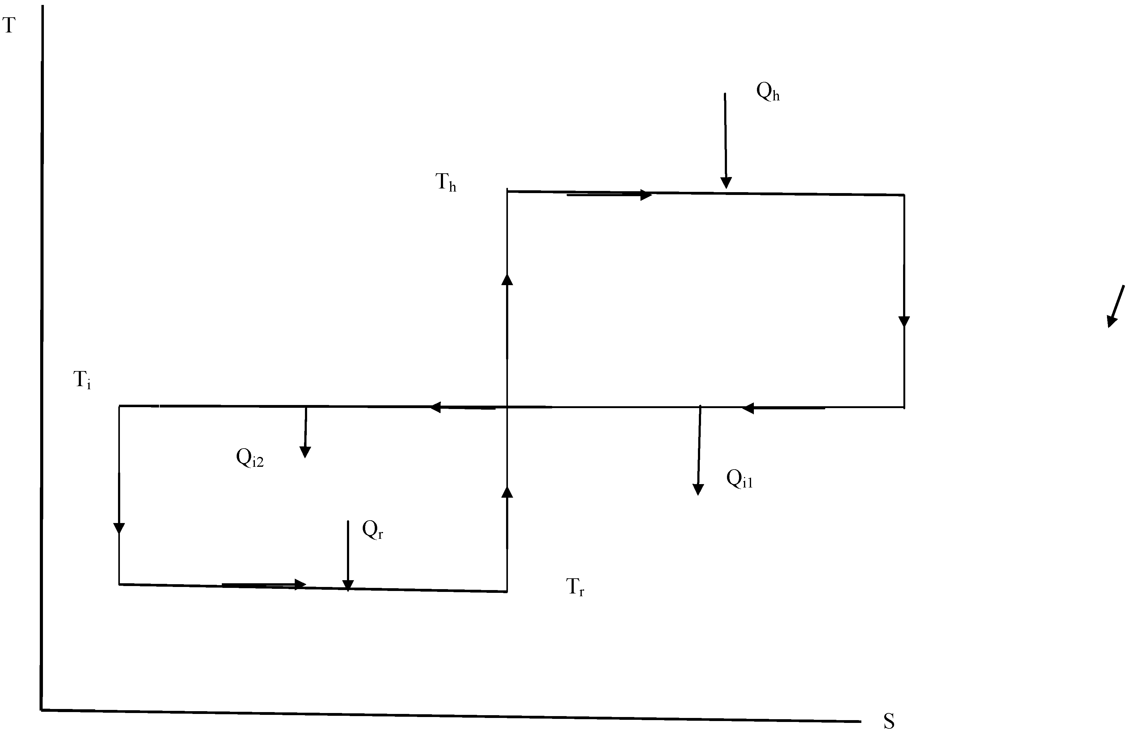
The Carnot tri-generation cycle which is depicted in Figure 2 consists of a power and refrigeration cycle coupled in such a manner that they have a common intermediate temperature Ti.
Figure 2.
T-S Diagram of a Carnot Tri-generation Cycle.

It is the purpose of a Tri-generation cycle to produce useful outputs of work, heating and cooling, so in this case since the refrigeration effect is a desired output the only external input will be Qh. The total output of the cycle will then be the network plus the refrigeration effect plus the heating effect:
To illustrate this energy accounting method consider the case of a supermarket that is using two electrically driven refrigeration cycles of the same performance to create a refrigeration effect and a heating effect. The overall coefficient of the refrigerator plus the heat pump will be equal to the coefficient of performance (COP) of the refrigerator plus one half. If the desired output can be produced from a single cycle (utilising both the refrigeration effect and the heating effect) the COP of this cycle will be double the COP of the two separate cycles. To put a value to this if the COP of the refrigeration cycle was to be 3 and that of the heat pump 4 the COP of the single cycle utilising all the output would be 7.
The useful output of the tri-generation cycle can be determined by considering the network expressed in terms of the heat transfer into and out of the cycle, (from the first law of thermodynamics), which is then added to the other useful energy outputs. The network is expressed as:
The total useful output of the cycle is then:
Which leads to the following:
and the efficiency is then:
and the EUF:
3.1. Finite Time Analysis
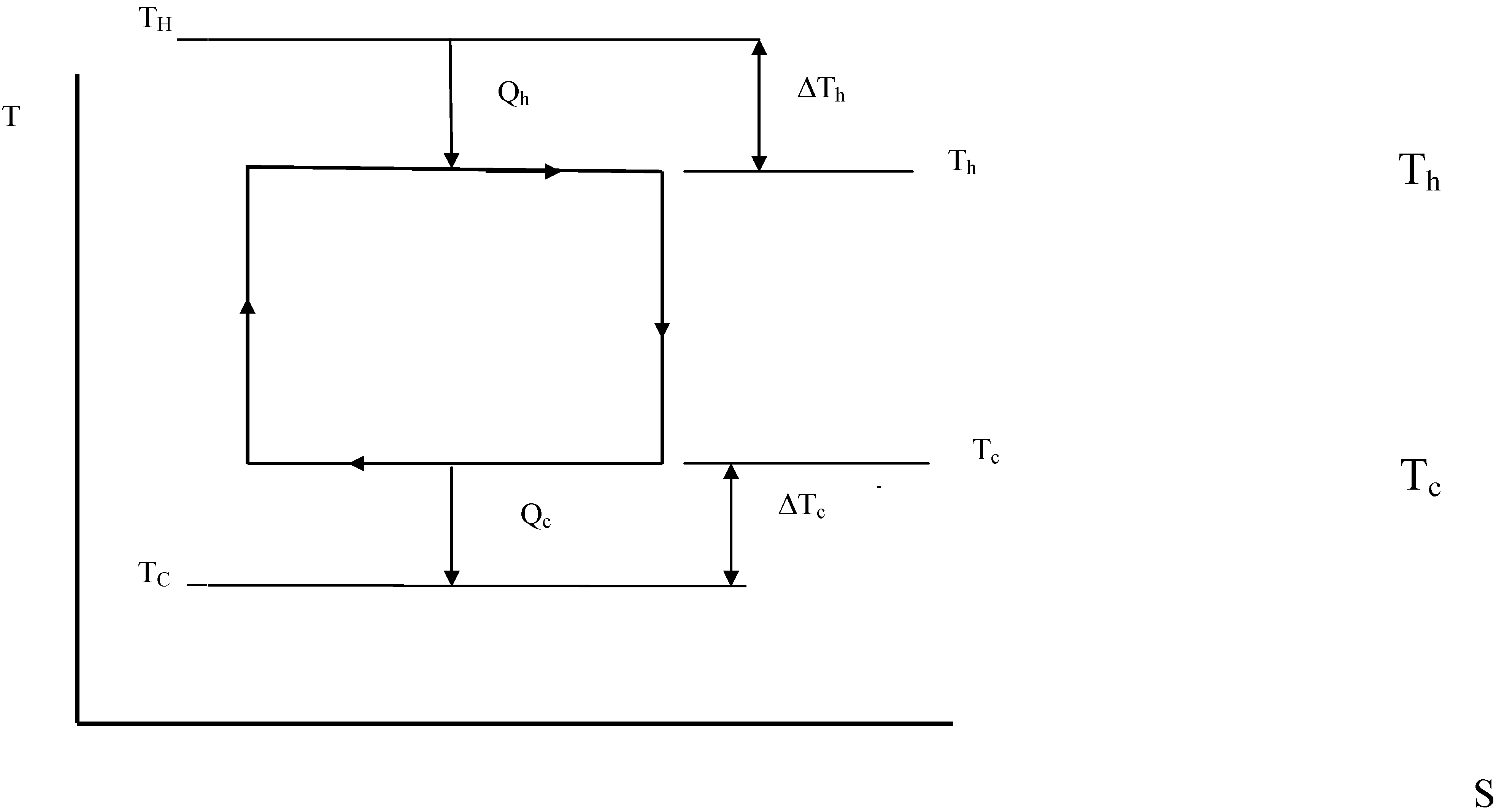
Finite time analysis of thermal systems produces a value of the overall efficiency that is close to that of real cycles [15,16] so acts as a yard stick by which real cycles may be judged. This analysis applies to internally reversible cycles that exchange heat energy between the environment through an isothermal convective heat transfer process. A temperature difference has been created between the cycle and the external reservoirs in order to increase the rate of heat transfer and also enable the cycle to have a high work rate or power output. This is shown in Figure 3.
Figure 3.
Finite Time TS Diagram of a Carnot Cycle.

It is assumed that the external thermal reservoirs are sufficiently large that they are maintained at a constant temperature and that the cycle energy exchange processes are also isothermal.
The rate of heat transfer between the cycle and the reservoirs can then be expressed as:
where h is the local heat transfer coefficient, A the heat transfer area and ΔT the temperature difference between the cycle and the reservoir. For a generalised steady flow cycle the first law of thermodynamics can be used to produce an expression for the cycle net-power output P:
Remembering that for the cycle:
then this becomes:
Either or can be eliminated by rearrangement, identical results being obtained in either case, e.g.:
Eliminating or produces the following equations:
It has been shown that θc is equal to θh at the maximum power condition [16] and for a fixed standard of heat exchanger performance (defined by constant values of and):
The cycle efficiency is then given by:
which becomes for the condition of maximum power:
This is the same as the result obtained by Curzon and Ahlborn [3] in their studies of a non-flow Carnot cycle.
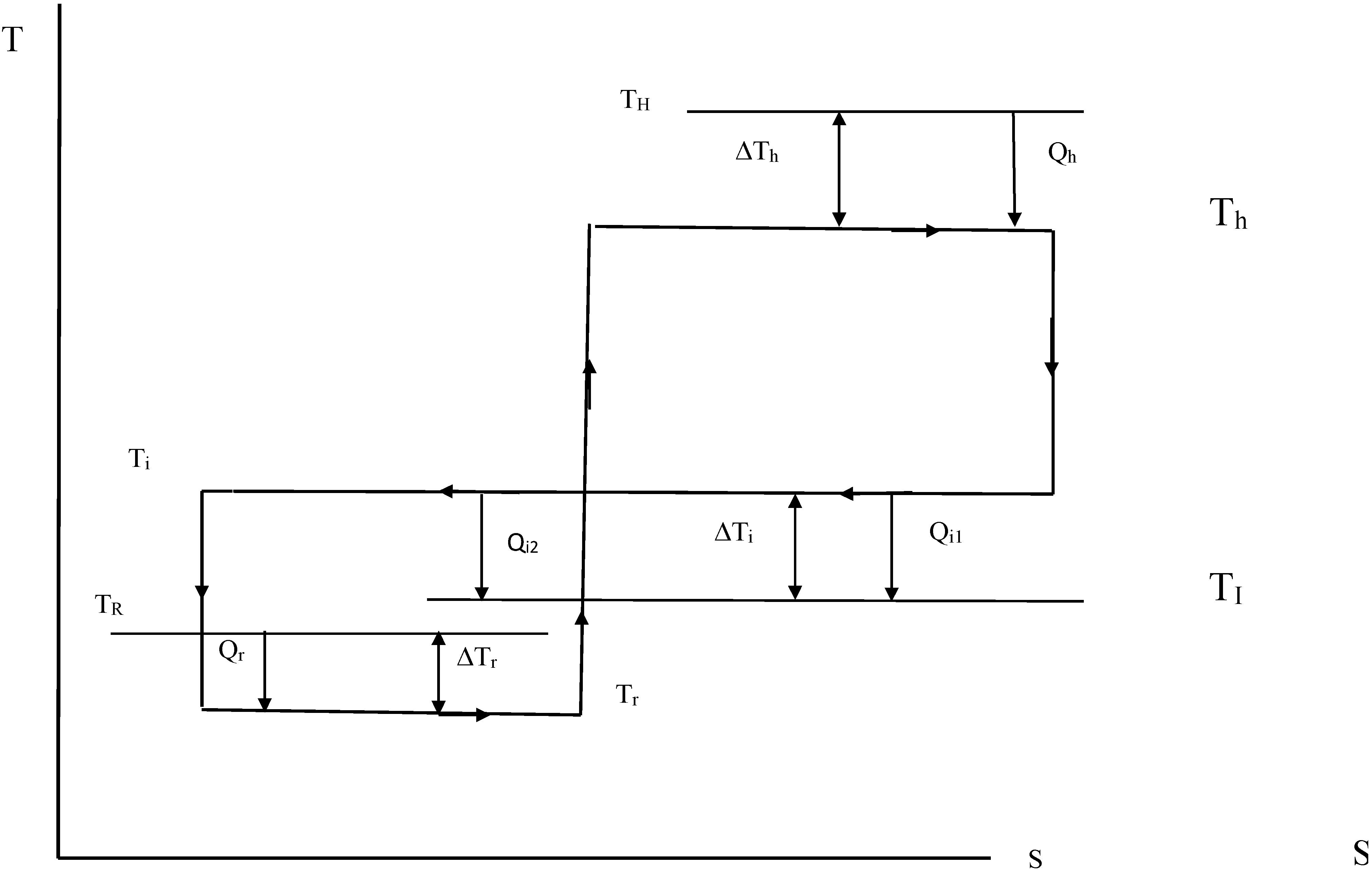
3.2. Tri-Generation Cycle
These equations have been applied to the Tri-generation cycle shown in Figure 4 that consists of coupled power and refrigeration cycles. It is assumed that applies for the whole of the heat rejection process at this part of the coupled cycles and is determined from the COP relationship of the refrigeration cycle. The temperature difference for the refrigeration effect is then:
Figure 4.
Finite-Time T-S diagram of a tri-generation Stirling cycle.

The analysis thus far has considered power and cooling cycles with equal volume ratios but it may be desirable for the cycle to be configured to produce external power as this has a greater utilisation capacity than heat or cooling. For instance it may be beneficial to utilise the output power to drive a vapour refrigeration cycle with a higher COP than could be produced by the cooling element of the tri-generation cycle. The tri-generation cycle can be biased towards power production or the production of heating and cooling by allowing the volume ratio of the refrigeration cycle to be different to that of the power cycle. This is equivalent to having different heat transfer areas between the power and the cooling cycles in Equation (8). The ratio of the volume ratio of the refrigeration cycle to that of the power cycle is denoted as x which is also the ratio of the heat transfer factors. If the cycle output is directed to power production the value of x would be less than one but if the cycle is directed towards production of heating and cooling then x will be greater than 1 subject to the condition that the output from the power cycle is sufficient to energise the refrigeration cycle. The net power and the heat transfer effects can be expressed as follows:
and the efficiency becomes:
and the EUF:
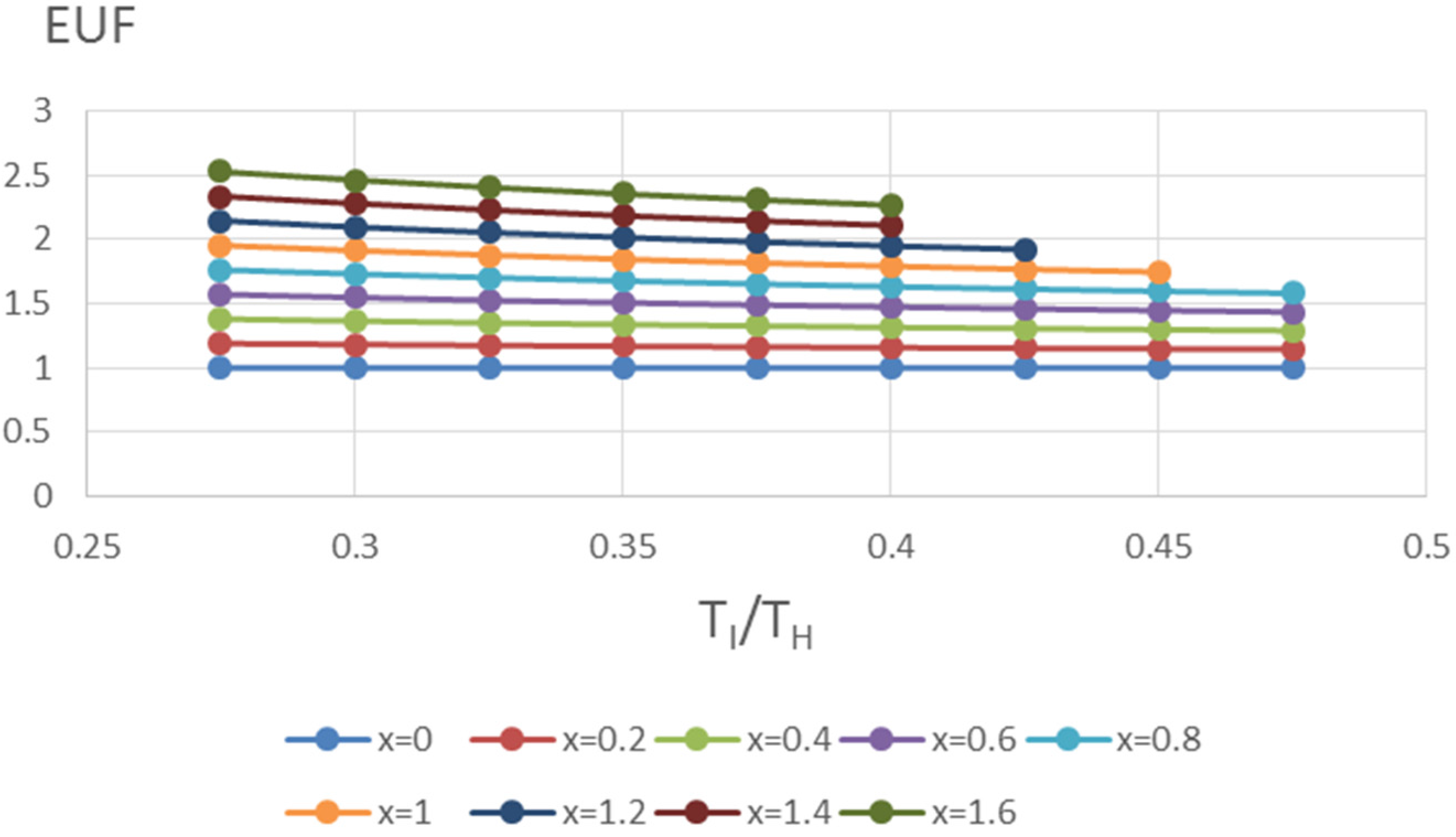
If the maximum and minimum reservoir temperatures, TH and TC are specified then the intermediate temperature TI is free to take any value between these subject to the condition that TI < TH and Tr < TR. The impact this has on the cycle output is shown in Figure 5, Figure 6 and Figure 7, which show the refrigeration and heating effects, net-power output as a proportion of the external heat input, and the EUF, plotted against TI/TH for different values of x and for TH = 1000 K and TR = 250 K. Figure 8 and Figure 9 indicate the impact that changing TH has on the cycle performance with TR set at 250 K.
Figure 5.
Tri-generation Cycle Efficiency with Respect to Intermediate Temperature Ratio and Volume Ratio, TR = 250 K, TH = 1000 K.
Figure 5.
Tri-generation Cycle Efficiency with Respect to Intermediate Temperature Ratio and Volume Ratio, TR = 250 K, TH = 1000 K.

Figure 6.
Tri-generation Cycle EUF with Respect to Intermediate Temperature Ratio and Volume Ratio, TR = 250 K, TH = 1000 K.
Figure 6.
Tri-generation Cycle EUF with Respect to Intermediate Temperature Ratio and Volume Ratio, TR = 250 K, TH = 1000 K.

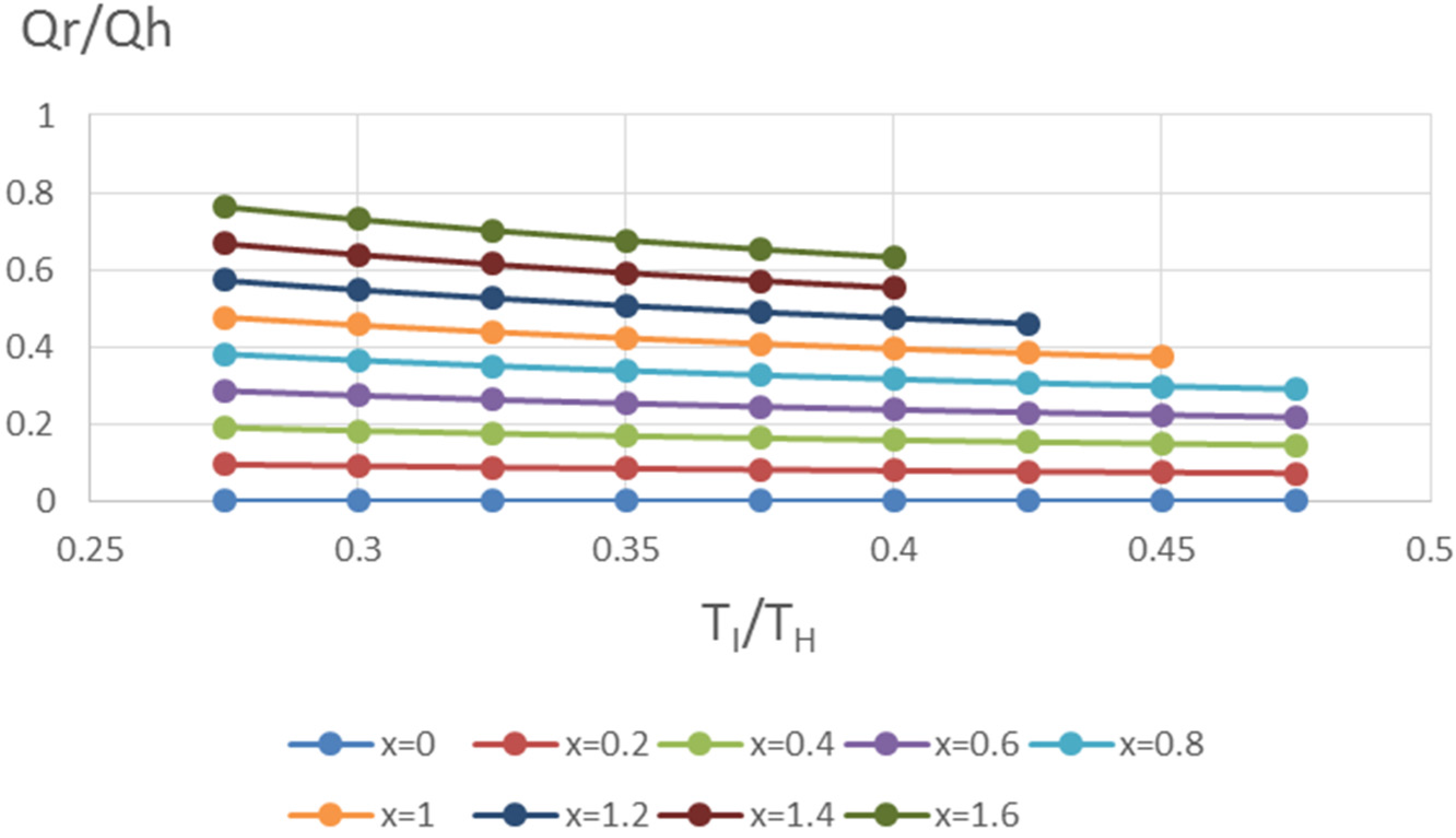
Figure 7.
Tri-generation Cycle Refrigeration Effect with Respect to Intermediate Temperature Ratio and Volume Ratio, TR = 250 K, TH = 1000 K.
Figure 7.
Tri-generation Cycle Refrigeration Effect with Respect to Intermediate Temperature Ratio and Volume Ratio, TR = 250 K, TH = 1000 K.

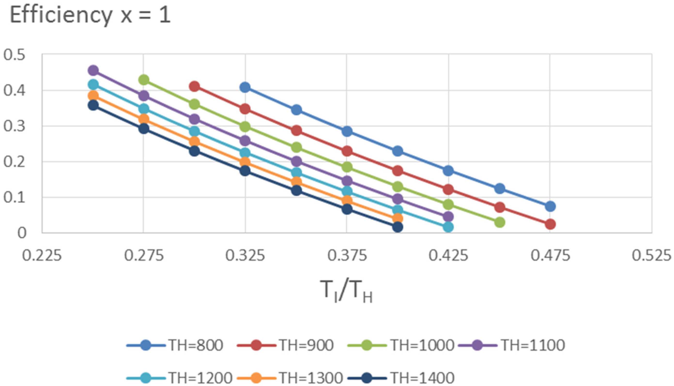
Figure 8.
Tri-generation Cycle Efficiency Respect to Intermediate Temperature Ratio and TH for x = 1, TR = 250 K.
Figure 8.
Tri-generation Cycle Efficiency Respect to Intermediate Temperature Ratio and TH for x = 1, TR = 250 K.

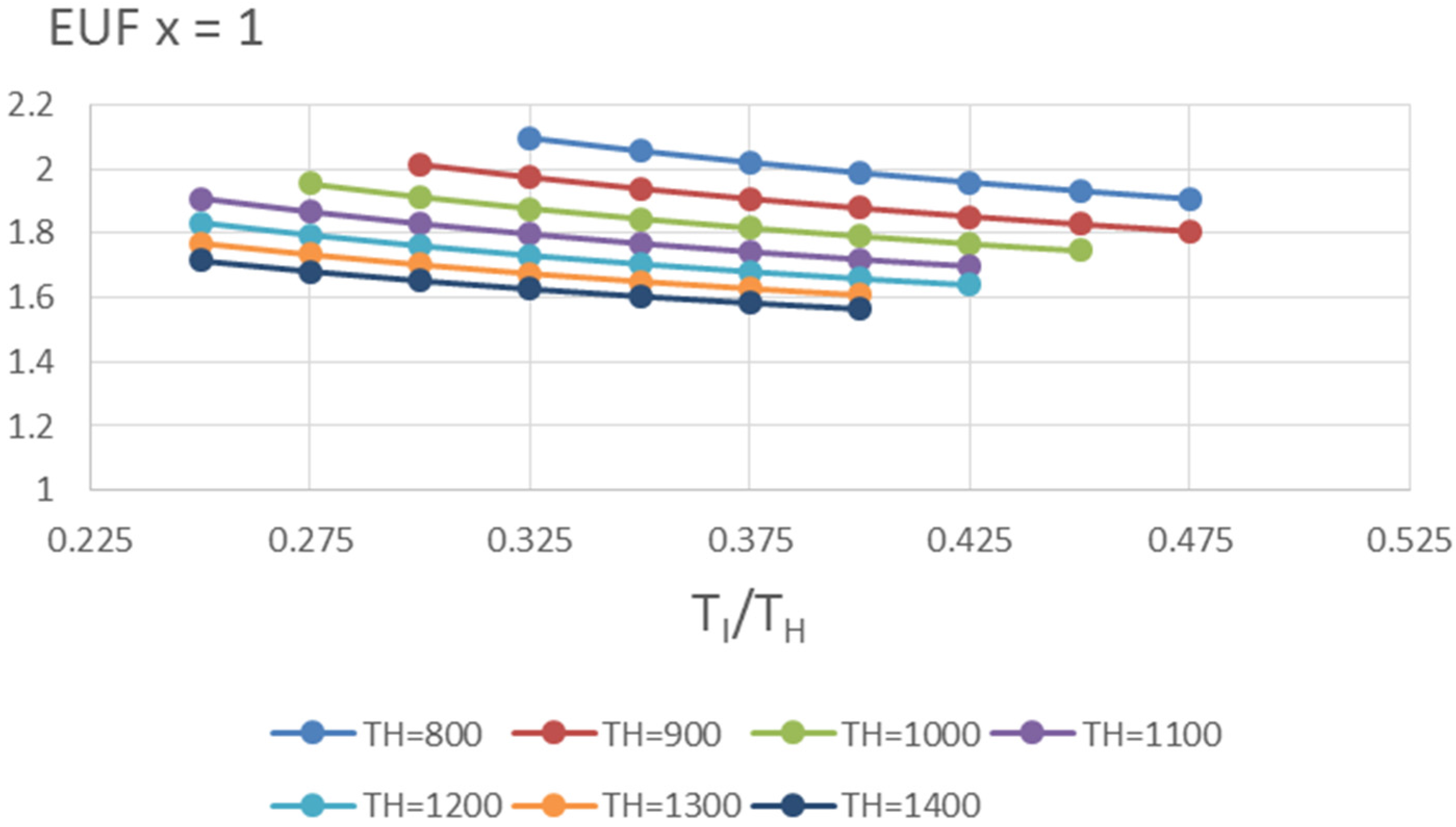
Figure 9.
Tri-generation Cycle EUF with Respect to Intermediate Temperature Ratio and TH for x = 1 and TR = 250 K.
Figure 9.
Tri-generation Cycle EUF with Respect to Intermediate Temperature Ratio and TH for x = 1 and TR = 250 K.

4. Discussion of Results
The performance of the tri-generation cycle has been depicted in the preceding graphs for a wide range of operating parameters. The impact of varying the ratio of the volume ratios of the two cycles, x, is very evident. When x = 0 the cycle is acting as a standalone CHP cycle producing net power and heating only. For all conditions examined the EUF in this state is equal to 1 as shown in Equation (24) and all the output is considered to be useful. The graphs have been truncated because the operating points go beyond those permissible by the constraints mentioned earlier.
The efficiency lines of Figure 5 all tend towards the point where the efficiency is 0.5, this is the same as the efficiency of the Finite Time Carnot cycle operating between TH = 1000 K and TC = 250 K but with an EUF of 1. This is the limit where TI = TR. The curves of the graphs shown in Figure 5 and Figure 8 intercept the x axis when the tri-generation cycle ceases to produce external power so is then functioning as a heat pump only as the generated power is entirely consumed by the refrigeration cycle. In the other graphs the curves are stopped at this point. The efficiency of the cycle is maximised when it is operating as a power cycle alone with an EUF of 1. A point of interest is the EUF values when the efficiency is zero. Taking values from Figure 6, TI/TH = 0.39, x = 1.6 and EUF = 2.26, the value of EUF is low compared with the COP of the vapour compression refrigerator referred to previously. The performance of the tri-generation cycle is inferior to that of an efficient electrical generator and a vapour compression refrigerator which raises the question of the suitability of this type of cycle for producing a refrigeration effect. The EUF values, however, are larger than those quoted in the literature for practical tri-generation cycles.
The cycle does not exhibit a maximum EUF condition but tends towards a maximum when TI/TH is lowest as shown in Figure 6. This is due to the condition that ΔTr, which is a function of TH, TR and TI, does not change with TH. This results in the refrigeration effect and the expansion work of the refrigeration process being a larger proportion of external heat input as TH is reduced. Also the heat rejected by the power cycle and the compression work associated with this energy transfer as a proportion of the heat input are constant. Both these factors have the effect of increasing the cycle efficiency and EUF as TH is reduced as can be seen in Figure 8 and Figure 9.
5. Conclusions
The performance of the tri-generation cycle, in terms of energy utilisation is improved as the temperature of the high temperature reservoir decreases. This marks the cycle as suitable for utilising waste heat. Maximum net-power output increases as TI is reduced at the expense of reducing the heat output as would be expected from a Carnot cycle. The refrigeration effect is less sensitive to the intermediate temperature and the EUF is highest when the cycle is operating at low temperatures and biased towards refrigeration. The values of EUF are typical of the values suggested by Horlock [2]. The performance of practical tri-generation cycles which utilise only low temperature energy derived from the primary energy input is reported to be very low when compared with an ideal cycle. This is probably due to internal irreversibility (low component performance) but is also due to the lack of interaction with the environment as described above. A finite time analysis of a Carnot cycle based tri-generation cycle shows much higher energy utilisation factors and indicates that the cycle is suitable when a low temperature energy supply is available. Of the three outputs of the cycle, the most abundant is waste heat which can be sacrificed for network and refrigeration effect. This analysis indicates that higher values of EUF can be produced in practice with innovatively designed cycles optimised for a particular application. This paper also indicates the dilemma facing the adoption of combined cycles for cooling purposes. As shown it can be more effective thermodynamically to focus on power generation and to use a proportion of this to drive a vapour compression refrigerator with a high COP (typically 3) than to use the heat to drive an absorption refrigerator with a low COP (typically 0.7). This is a question that thermodynamics alone cannot answer as the economics of a particular plant and lifetime running costs may have some bearing on this.
Acknowledgments
The authors gratefully acknowledge the constructive and insightful comments received from the reviewers.
Author Contributions
This paper developed from an idea discussed by Brain Agnew and Ivan C. K. Tam in the summer of 2014 by Sara Walker and Bobo Ng who were working in the Building services group at Northumbria University with Brain Agnew. It is based on Finite Time Thermodynamics that was a topic of interest of Agnew and Tam in the 1990s. The development of these ideas to the tri-generation cycle was done by Sara Walker and Bobo Ng and Ivan C. K. Tam. The final version taking into account the comments of the referees was developed by Brain Agnew.
Conflicts of Interest
The authors declare no conflict of interest.
Nomenclature
| A | Effective heat transfer area m2 |
| eff | Thermal Efficiency, Network/Primary heat input |
| effp | Efficiency at maximum power condition |
| EUF | Energy utilisation factor; Useful output/Primary input |
| h | Heat transfer coefficient W/m2K |
| P | Net power output W |
| Q | Heat transfer J; Heat transfer rate W |
| Qh | Primary Energy input i.e., that provided from an external source at a financial cost. |
| R | Specific gas constant J/kgK |
| S | Entropy J/kgK |
| T | Temperature K |
| T0 | Heat sink temperature |
| vr | Volume ratio |
| x | Ratio of volume ratios, cooling cycle vr/power cycle vr |
| ΔT | Temperature difference K |
| θ | hA W/K |
| Subscripts | |
| C, c | Low temperature isotherm of Stirling cycle |
| H, h | High temperature |
| I, i | Intermediate temperature |
| R, r | Refrigeration temperature |
| Upper case refers to external reservoir temperature; lower case refers to cycle isotherm | |
References
- Horlock, J.H. Approximate Analysis of Feed and District Heating Cycles for Steam Combined Heat and Power. Proc. Inst. Mech. Eng. Part A: J. Power Energy 1987, 201, 193–200. [Google Scholar] [CrossRef]
- Horlock, J.H.; Haywood, R.W. Thermodynamic Availability and its Application to Combined Heat and Power Plant. Proc. Inst. Mech. Eng. Part C: J. Mech. Eng. Sci. 1985, 199, 11–17. [Google Scholar] [CrossRef]
- Curzon, F.L.; Ahlborn, B. Efficiency of a Carnot Engine at Maximum Power Output. Am. J. Phys. 1975, 43, 22–24. [Google Scholar] [CrossRef]
- Leff, H.S. Thermal efficiency at Maximum Work Output; New Results for Old Engines. Am. J. Phys. 1987, 55, 602–610. [Google Scholar] [CrossRef]
- Salamon, P.; Nitzan, A. Finite Time Optimisation of a Newton’s law Carnot Cycle. J. Chem. Phys. 1981, 74, 3546–3560. [Google Scholar] [CrossRef]
- Gordon, J.M. Maximum Power Point Characteristics of Heat Engines as a General Thermodynamic Problem. Am. J. Phys. 1989, 57, 1136–1142. [Google Scholar] [CrossRef]
- Swanson, L.W. Thermodynamic Optimisation of Irreversible Power Cycles with Constant External Reservoir Temperatures. ASME J. Eng. Gas Turbine Power 1991, 113, 505–510. [Google Scholar] [CrossRef]
- Salamon, P.; Band, Y.B.; Kafri, O. Maximum Power from a Cycling Working Fluid. J. Appl. Phys. 1982, 53, 197–202. [Google Scholar] [CrossRef]
- Rozonoer, L.I.; Tsitlin, A.M. Optimal Control of Thermodynamic Processes. Autom. Remote Control 1983, 44, 314–321. [Google Scholar]
- Kaushik, S.C.; Tyagi, S.K.; Bose, S.K.; Singhal, M.K. Performance Evaluation of Irreversible Stirling and Ericsson Heat Pump cycles. Int. J. Therm. Sci. 2002, 41, 193–200. [Google Scholar] [CrossRef]
- Ondrechen, M.J.; Andersen, B.; Mozurkiewicz, M.; Berry, M.S. Maximum Work from a Finite Reservoir by Sequential Carnot Cycles. Am. J. Phys. 1981, 49, 681–685. [Google Scholar] [CrossRef]
- Pinho, C. The Curzon-Ahlborn Efficiency of Combined Cycles. In Proceedings of the 17th International Congress of Mechanical Engineering, Sao Paulo, Brazil, 10–14 November 2003.
- Sieniutycz, S. Optimal Work in Sequential Systems with Complex Heat Exchange. Int. J. Heat Mass Transf. 2001, 44, 897–918. [Google Scholar] [CrossRef]
- Agnew, B.; Alikitiwi, A.; Anderson, A.A.; Fisher, E.H.; Potts, I. A Finite Time Analysis of Combined Carnot Driving and Cooling Cycles Optimised for Maximum Refrigeration Effect with Applications to Absorption Refrigeration Systems. Exergy Int. J. 2002, 2, 186–191. [Google Scholar] [CrossRef]
- Bejan, A. Advanced Engineering Thermodynamics; Wiley: New York, NY, USA, 1988. [Google Scholar]
- Agnew, B.; Anderson, A.; Frost, T.H. Optimisation of a Steady Flow Carnot Cycle with External Irreversibility for Maximum Specific Output. Appl. Therm. Eng. 1997, 17, 3–15. [Google Scholar] [CrossRef]
- Maloney, J.D.; Robertson, R.C. Thermodynamic Study of Ammonia-Water Heat Power Cycles; Oak Ridge National Laboratory: Oak Ridge, TN, USA, 1953.
- Kalina, A.I.; Tribus, M. Advances in Kalina Cycle Technology (1980–1991): Part I Development of a Practical Cycle. In Proceedings of the Florence World Energy Research Symposium, Firenze, Italy, 7–12 June 1992.
- Xu, F.; Goswami, D.Y. Thermodynamic Properties of Ammonia-Water Mixtures for Power Cycle Applications. Energy 1999, 24, 525–536. [Google Scholar] [CrossRef]
- Tassou, S.A.; Chaer, I.; Suguartha, N.; Ge, T.; Marriott, D. Application of Tri-generation Systems to the Food Retail Industry. Energy Convers. Manag. 2007, 48, 2988–2995. [Google Scholar] [CrossRef]
- Ameri, M.; Behbahaninia, A.; Tanha, A.A. Thermodynamic Analysis of a Tri-generation System Based on Micro-gas Turbine with a Steam Ejector Refrigeration System. Energy 2010, 35, 2203–2209. [Google Scholar] [CrossRef]
- Meunier, F.; Chevalier, C. Environmental Assessment of Biogas Co- or Tri-generation Units by Life Cycle Analysis Methodology. Appl. Therm. Eng. 2005, 25, 3025–3041. [Google Scholar]
- Meunier, F. Co-and Tri-generation Contribution to Climate Change Control. Appl. Therm. Eng. 2002, 22, 703–718. [Google Scholar] [CrossRef]
- Godefroy, J.; Riffat, S.B.; Worall, M.; Boukhanouf, R. Design and Optimisation of a Small-scale Tri-generation System. Int. J. Low-Carbon Technol. 2008, 3, 32–43. [Google Scholar]
- Chen, X. Integration and Optimisation of Bio-fuel Micro Tri-generation with Energy Storage. Ph.D. Thesis, Newcastle University, Newcastle upon Tyne, UK, 2013. [Google Scholar]
- Glavan, I.; Prelec, Z. The Analysis of Trigeneration Energy Systems and Selection of the Best Option Based on Criteria of GHG Emission, Cost and Efficiency. Eng. Rev. 2012, 32, 131–139. [Google Scholar]
© 2015 by the authors; licensee MDPI, Basel, Switzerland. This article is an open access article distributed under the terms and conditions of the Creative Commons Attribution license (http://creativecommons.org/licenses/by/4.0/).
Share and Cite
MDPI and ACS Style
Agnew, B.; Walker, S.; Ng, B.; Tam, I.C.K. Finite Time Analysis of a Tri-Generation Cycle. Energies 2015, 8, 6215-6229. https://doi.org/10.3390/en8066215
AMA Style
Agnew B, Walker S, Ng B, Tam ICK. Finite Time Analysis of a Tri-Generation Cycle. Energies. 2015; 8(6):6215-6229. https://doi.org/10.3390/en8066215
Chicago/Turabian StyleAgnew, Brian, Sara Walker, Bobo Ng, and Ivan C. K. Tam. 2015. "Finite Time Analysis of a Tri-Generation Cycle" Energies 8, no. 6: 6215-6229. https://doi.org/10.3390/en8066215