Model-Based State Feedback Controller Design for a Turbocharged Diesel Engine with an EGR System

Abstract

This paper describes a method for the control of transient exhaust gas recirculation (EGR) systems. Firstly, a state space model of the air system is developed by simplifying a mean value model. The state space model is linearized by using linearization theory and validated by the GT-Power data with an operating point of the diesel engine. Secondly, a state feedback controller based on the intake oxygen mass fraction is designed for EGR control. Since direct measurement of the intake oxygen mass fraction is unavailable on the engine, the estimation method for intake oxygen mass fraction has been proposed in this paper. The control strategy is analyzed by using co-simulation with the Matlab/Simulink and GT-Powers software. Finally, the whole control system is experimentally validated against experimental data of a turbocharged diesel engine. The control effect of the state feedback controller compared with PID controller proved to be further verify the feasibility and advantages of the proposed state feedback controller.

1. Introduction

Increasing demands for more efficient engines and stringent limits on exhaust gas pollution require more accurate control of engine operating parameters, especially under transient conditions. EGR is an effective technology to reduce NOx emissions from diesel engines. The traditional EGR control can be divided into open loop control and closed loop control. In open loop control, according to the current conditions and the steady-state control MAP, the EGR valve opening is adjusted by the control system. This control method is simple, but has low precision because the engine operation parameter variation under transient conditions are not considered. In order to improve the control precision, the closed loop EGR control system was developed and tested. The closed loop EGR control mainly includes two categories, EGR valve opening control and EGR rate control. For the EGR valve opening control, according to the MAP of EGR rate, the optimum EGR rate with certain conditions is calculated by the control system. Based on the EGR valve opening MAP, the target EGR valve opening is calculated. Finally, based on the target and actual EGR valve opening, the EGR valve is controlled by a PID controller. This control mode is more common because it has good control effects under steady-state conditions, but under transient condition, EGR valve opening cannot completely reflect the real EGR rate, so it is unable to realize an accurate EGR rate control. For the EGR rate control, the EGR rate estimation method based on the air flow is often used [1]. The target EGR rate is identified firstly by the control system based on the EGR rate MAP, then the target air flow is calculated based on the air flow MAP, finally, according to the desired and real air flow, the EGR valve is controlled by a PID controller. In this control mode, it is assumed that the amount of intake gas does not change under certain conditions, however, with the poor transient response of the turbocharger, the amount of intake gas will change a lot during transient conditions which may lower the control precision of the EGR rate.

The traditional EGR control method without fully considering the properties of inertial components under transient operation conditions makes the EGR system unable to operate with optimum behavior under transient conditions, which may result in a deterioration of the transient emissions. Research on transient EGR control has been presented in recent years [2,3,4,5,6], most of which control methods are based on PID output feedback control algorithms. The EGR rate, excess air coefficient and intake oxygen concentration are often adopted as feedback parameters. With the development of modern control theory, more and more new control algorithm have gradually been applied in diesel engine air system control (EGR control and variable geometry turbocharger or VGT control), such as model based predictive control [7], linear quadratic gaussion control [8], and the nonlinear Sliding Mode Control [9], etc. All these control methods improve the control precision and response properties of the controller. The state feedback control is the most basic control form of modern control theory. Compared to the traditional output feedback control, the state feedback control can effectively improve the performance of the system [10].

For the transient EGR control of the turbocharged diesel engine, because the control object is complex and the control requirements are very high, new control methods are needed. In this paper, a method based on state feedback control is proposed to control EGR systems. Firstly, the dynamic model of the air system is developed. Then according to the control requirements, the model is simplified. After that, the model is linearized according to the linear theory. Using the data simulated by a calibrated GT-Power model at a certain operation point, all these characteristics of the state space model (controllability, observability and stability), are analyzed. A state feedback controller based on the intake oxygen mass fraction has been designed to control the EGR system. Since the intake oxygen mass fraction cannot be measured directly, a method to estimate the intake oxygen mass fraction has been proposed in this paper. The control strategy is evaluated by using a co-simulation with GT-Power and Matlab/Simulink. Finally, the designed controller is tested on a light-duty turbocharged diesel engine with an EGR system. Compared with the PID controller, the control effects of the state feedback controller are greatly improved and the performance of the state feedback controller is verified by the experimental results.

2. Dynamic Model

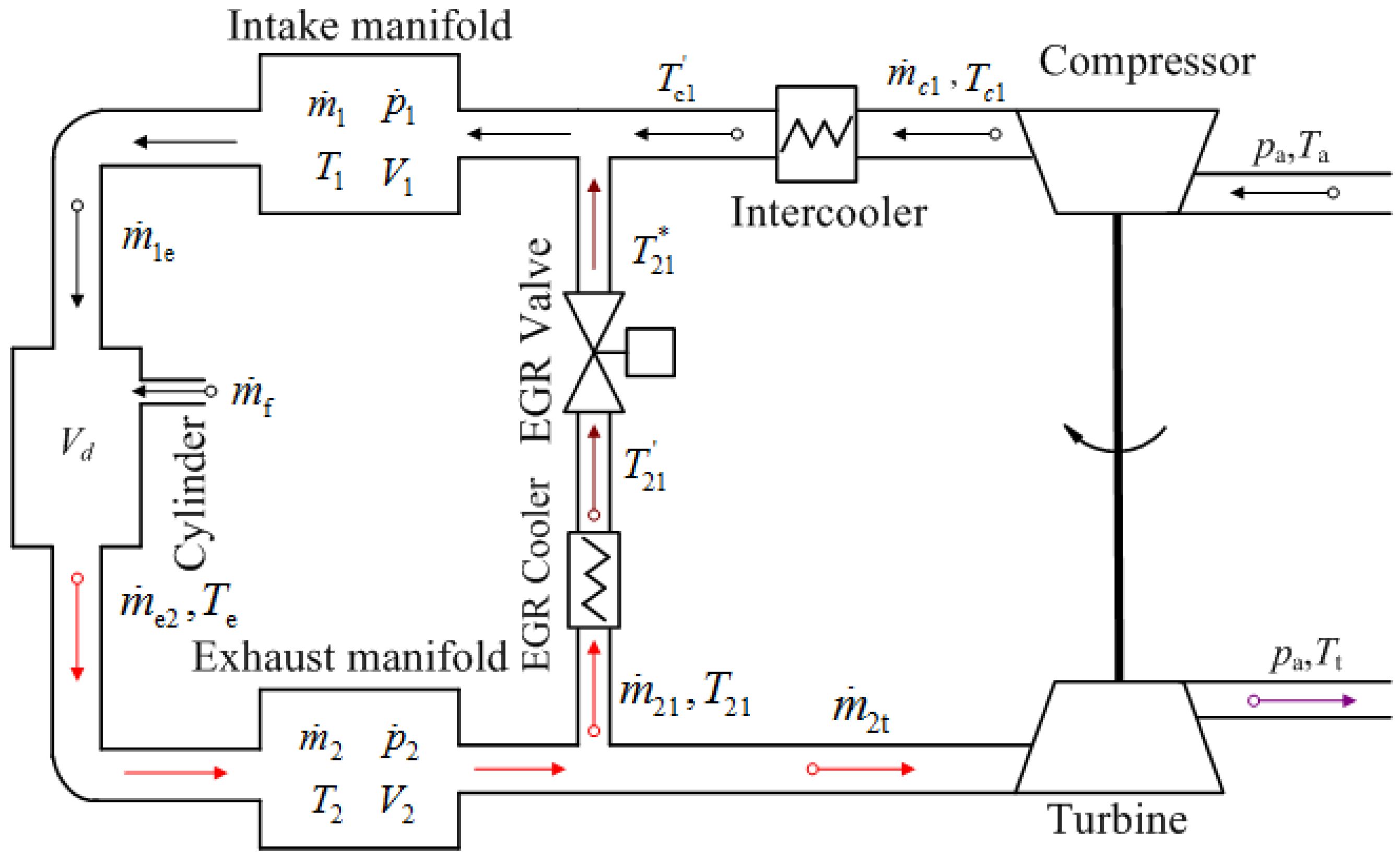
In this paper, the mean value model is developed by using the YC4E170-31 turbocharged diesel engine as a prototype engine. Matlab/Simulink is used as the tool to build the model. The diesel engine system consists of the intake manifold, exhaust manifold, turbocharger, EGR valve, intercooler, EGR cooler and cylinder, as shown in Figure 1. Detailed descriptions of all these subsystems are given in the following sections.

Figure 1. Block diagram of turbocharged diesel engine with HP EGR system.

Figure 1. Block diagram of turbocharged diesel engine with HP EGR system.

2.1. Intake Manifold

Generally, the control volume method is used to build the intake manifold model. It is assumed that the intake manifold temperature is constant, according to the conservation of mass and energy and the ideal gas law, the gas mass, pressure, and air mass fraction of the intake manifold can be derived as [11]:

$${\dot{m}}_{\text{1}}={\dot{m}}_{\text{c1}}+{\dot{m}}_{\text{21}}-{\dot{m}}_{\text{1e}}$$

(1)

$${\dot{p}}_1=\frac{\text{γ}{R}_{\text{g}}}{V_1}\left({\dot{m}}_{\text{c1}}{T}_{\text{c}1}^{\prime }+{\dot{m}}_{\text{21}}{T}_{21}^{\prime }-{\dot{m}}_{\text{1e}}{T}_1\right)$$

(2)

$${\dot{F}}_1=\frac{{\dot{m}}_{21}\left(F_2-F_1\right)+{\dot{m}}_{\text{c1}}\left(1-F_1\right)}{m_1}$$

(3)

where ${\dot{m}}_{\text{c1}}$ is the gas flow rate through the compressor; ${\dot{m}}_{21}$ is the gas flow rate through the EGR valve; ${\dot{m}}_{\text{1e}}$ is the gas flow rate into the cylinder; ${\dot{m}}_1$ is the gas flow rate through the intake manifold; m₁ is the gas mass in the intake manifold; $T_{\text{c1}}^{\text{′}}$ is the outlet temperature of intercooler; $T_{21}^{\prime }$ is the inlet temperature of EGR valve; V₁ is the volume of the intake manifold; γ is the specific heat ratio of the air in the intake manifold; R_g is the gas constant of air in the intake manifold; F₂ is the air mass fraction of the unburned air in the exhaust manifold; F₁ is the total air-mass fraction in the intake manifold.

2.2. Exhaust Manifold

The exhaust manifold is modeled in the same way as the intake manifold:

$${\dot{m}}_2={\dot{m}}_{\text{e2}}-{\dot{m}}_{\text{21}}-{\dot{m}}_{\text{2t}}$$

(4)

$${\dot{p}}_2=\frac{\text{γ}{R}_{\text{g}}}{V_2}\left({\dot{m}}_{\text{e2}}{T}_{\text{e}}-{\dot{m}}_{\text{21}}{T}_2-{\dot{m}}_{\text{2t}}{T}_2\right)$$

(5)

$${\dot{F}}_2=\frac{{\dot{m}}_{\text{e2}}\left(F_{\text{e2}}-F_2\right)}{m_2}$$

(6)

where ${\dot{m}}_{\text{e}2}$ is the mass flow of the exhaust from the cylinder; ${\dot{m}}_{\text{2t}}$ is the mass flow of gas through the turbine; m₂ is the mass of gas in the exhaust manifold; T_e, T₂ are the temperature of the gas exhaust from cylinder, the gas in the exhaust manifold; F_e2 is the mass fraction of unburned air exhausted from cylinder; V₂ is the volume of the exhaust manifold.

2.3. Turbocharger

Turbocharger can be simplified as a first order inertia system with a time constant [12]:

$${\dot{P}}_{\text{c}}=\frac{1}{{\text{τ}}_{\text{tc}}}\left({\text{η}}_{\text{m}}{P}_{\text{t}}-P_{\text{c}}\right)$$

(7)

where η_m is the turbocharger mechanical efficiency; τ_tc is a time constant associated with the structure of the turbocharger. The output power of turbine can be estimated based on the first law of thermodynamics [13,14]:

$$P_{\text{t}}={\text{η}}_{\text{t}}{\dot{m}}_{\text{2t}}{c}_{\text{p,2}}{T}_2\left(1-{\text{π}}_{\text{t}}^{\frac{1-\text{γ}}{\text{γ}}}\right)$$

(8)

Similarly, the flow of the compressor can be approximated by:

$${\dot{m}}_{\text{c1}}=\frac{P_{\text{c}}{\text{η}}_{\text{c}}}{c_{\text{p,1}}{T}_{\text{a}}\left({\text{π}}_{\text{c}}^{\frac{\text{γ}-1}{\text{γ}}}-1\right)}$$

(9)

where π_t = p₂/p_a is the expansion ratio of turbine; π_c = p₁/p_a is the boost pressure ratio of compressor; η_t, η_c are the isoentropic efficiency of turbine and compressor respectively. The mass flow of the turbine can be estimated based on the equation of continuity of gas steady flow [5]:

$${\dot{m}}_{2t}=\frac{A_{\text{eff}}{p}_2}{\sqrt{R_{\text{g}}{T}_2}}{\text{ψ}}_{\text{t}}\left(p_{\text{a}},p_2\right)$$

(10)

where ${\text{ψ}}_{\text{t}}\left(p_{\text{a}},p_2\right)=\{\begin{array}{l}\frac{1}{\sqrt{2}},0\le \frac{p_{\text{a}}}{p_2}<0.5\\ \sqrt{\frac{2p_{\text{a}}}{p_2}\left(1-\frac{p_{\text{a}}}{p_2}\right)},0.5\le \frac{p_a}{p_2}<1\end{array}$, A_eff is effective flow area of the turbine nozzle.

The outlet temperature of the compressor can be calculated as [15]:

$$T_{\text{c1}}=T_{\text{a}}\left[1+\frac{1}{{\text{η}}_{\text{c}}}\left({\text{π}}_{\text{c}}^{\frac{\text{γ}-1}{\text{γ}}}-1\right)\right]$$

(11)

2.4. EGR Valve

The EGR flow rate can be approximately calculated by a nozzle orifice equation, and can be simplified as follows:

$${\dot{m}}_{21}=\frac{A_{\text{egr}}{p}_2}{\sqrt{R_{\text{g}}{T}_{21}^{\prime }}}{\text{ψ}}_{\text{e}}\left(p_1,p_2\right)$$

(12)

where ${\text{ψ}}_{\text{e}}\left(p_1,p_2\right)=\{\begin{array}{l}\frac{1}{\sqrt{2}},0\le \frac{p_1}{p_2}<0.5\\ \sqrt{\frac{2p_1}{p_2}\left(1-\frac{p_1}{p_2}\right)},0.5\le \frac{p_1}{p_2}<1\end{array}$, $A_{\text{egr}}=C_{\text{d}}\left(u_{\text{egr}}\right)A_{\text{ref}}$ is the effective flow area of the EGR valve, A_ref is the reference flow area of the EGR valve; C_d(u_egr) is the flow coefficient, which is the function of the EGR valve opening rate; $T_{21}^{\prime }$ is the temperature downstream of the EGR cooler.

2.5. Coolers

There are two coolers in the whole system: the intercooler and the EGR cooler. Usually the pressure drops across the coolers are neglected, and the temperatures after the coolers can be calculated by the following equations [16]:

$$T_{\text{c1}}^{\prime }=T_{\text{c1}}\left(1-{\eta }_{c,c}\right)+{\text{η}}_{\text{c},\text{c}}{T}_{\text{cool}}$$

(13)

$$T_{\text{21}}^{\prime }=T_{21}\left(1-{\text{η}}_{\text{c},\text{e}}\right)+{\text{η}}_{\text{c},\text{e}}{T}_{\text{cool}}$$

(14)

where T_cool is the coolant temperature; η_c,c, η_c,e are the cooling efficiency of the intercooler and the EGR cooler.

2.6. Cylinder

As the research object is the air system of a diesel engine, the physical model of the cylinder can be relatively simple. The cylinder is simply treated as a material exchange channel for the intake manifold and the exhaust manifold. The dynamic characteristics of the cylinder are neglected, Assuming that the engine speed is as a known input, the mass flow into the cylinder can be calculated by speed density equation [17]:

$${\dot{m}}_{\text{1e}}=\frac{N_{\text{e}}{V}_{\text{d}}{p}_1}{120R_{\text{g}}{T}_1}{\text{η}}_{\text{vol}}$$

(15)

where N_e is the engine speed; V_d is the cylinder displacement volume; η_vol is the volumetric efficiency of the cylinder, which is a function of the engine speed and intake-exhaust pressure [18]. Regardless of the residual gas retention, mass flow of exhaust gas from cylinder can be calculated as follows:

$${\dot{m}}_{\text{e2}}={\dot{m}}_{\text{1e}}+{\dot{m}}_{\text{f}}$$

(16)

The mass fraction of unburned air in the exhaust gas can be calculated with the assumption that the fuel injected into the cylinder is completely burned:

$$F_{\text{e2}}=\frac{F_1{\dot{m}}_{\text{1e}}-l_0{\dot{m}}_{\text{f}}}{{\dot{m}}_{\text{e2}}}$$

(17)

where ${\dot{m}}_{\text{f}}$ is the mass flow of fuel; $l_0$ is stoichiometric air-fuel ratio.

The exhaust temperature T_e is affected by many factors which can be modeled by usually using steady state date fitting method:

$$\begin{array}{l}{T}_{\text{e}}=T_1+\mathrm{\Delta }{T}_{\text{e}}\\ \mathrm{\Delta }{T}_{\text{e}}=f_1(N,{\varphi }_{\text{a}},F_1)\end{array}\}$$

(18)

where ${\varphi }_{\text{a}}$ is the excess air coefficient.

2.7. Model of the Air System

Through the above analysis, the air system can be described by seven differential equations (Equation (19)):

$$\begin{array}{l}{\dot{m}}_{\text{1}}={\dot{m}}_{\text{c1}}+{\dot{m}}_{\text{21}}-{\dot{m}}_{\text{1e}}\\ {\dot{p}}_1=\frac{\text{γ}{R}_{\text{g}}}{V_1}\left({\dot{m}}_{\text{c1}}{T}_{\text{c}1}^{\prime }+{\dot{m}}_{\text{21}}{T}_{21}^{\prime }-{\dot{m}}_{\text{1e}}{T}_1\right)\\ {\dot{F}}_1=\frac{{\dot{m}}_{21}\left(F_2-F_1\right)+{\dot{m}}_{\text{c1}}\left(1-F_1\right)}{m_1}\\ {\dot{m}}_2={\dot{m}}_{\text{e2}}-{\dot{m}}_{\text{21}}-{\dot{m}}_{\text{2t}}\\ {\dot{p}}_2=\frac{\text{γ}{R}_{\text{g}}}{V_2}\left({\dot{m}}_{\text{e2}}{T}_{\text{e}}-{\dot{m}}_{\text{21}}{T}_2-{\dot{m}}_{\text{2t}}{T}_2\right)\\ {\dot{F}}_2=\frac{{\dot{m}}_{\text{e2}}\left(F_{\text{e2}}-F_2\right)}{m_2}\\ {\dot{P}}_{\text{c}}=\frac{1}{{\text{τ}}_{\text{tc}}}\left({\text{η}}_{\text{m}}{P}_{\text{t}}-P_{\text{c}}\right)\end{array}\}$$

(19)

There are seven states corresponding to these seven differential equations, and these states describe the mass, pressure and elements of the gas in the intake and exhaust manifold, and the dynamic characteristics of the turbocharger.

2.8. Model Simplification and Linearization

2.8.1. Model Simplification

The dynamic model given by Equation (19) is widely applied in analyzing the characteristics of air systems. As this model is too complex, there will be many limits when using the model to design a controller. Thus, the model should be simplified. According to the analysis of [19], it is more reasonable to select the intake oxygen mass fraction as the control parameter for EGR control. The oxygen mass fraction in the intake manifold and exhaust manifold can be calculated based on mass conservation:

$${\dot{X}}_{\text{O,1}}=\frac{\left(X_{\text{O,2}}-X_{\text{O,1}}\right){\dot{m}}_{\text{21}}+\left(X_{\text{O,air}}-X_{\text{O,1}}\right){\dot{m}}_{\text{c1}}}{m_1}$$

(20)

$${\dot{X}}_{\text{O,2}}=\frac{\left(X_{\text{O,e}}-X_{\text{O,2}}\right){\dot{m}}_{\text{e2}}}{m_2}$$

(21)

where X_O,air is the oxygen mass fraction of air. The oxygen mass fraction of the exhaust gas can be approximated by $X_{\text{O,e}}=\left({\dot{m}}_{1\text{e}}{X}_{\text{O,}1}-{\dot{m}}_{\text{f}}{l}_{\text{1}}\right)/{\dot{m}}_{\text{e}2}$, l₁ is the stoichiometric oxygen fuel ratio. Assuming that the temperature of the intake and exhaust gas not changed in transient condition, the intake and exhaust flow m₁ and m₂ can be calculated by the ideal gas equation [20], the two states can be removed from the model.

Selecting the state variables x = [p₁, p₂, X_O,1, X_O,2, P_c] and the input variable u = u_egr, the state space equation of the air system can be derived as:

$$\begin{array}{l}{\dot{p}}_1=-K_1{p}_1+K_2{C}_{\text{d}}(u_{\text{egr}}){\text{ψ}}_{\text{e}}{p}_2+\frac{K_3}{\left({\text{π}}_{\text{c}}^{\frac{\text{γ}-1}{\text{γ}}}-1\right)}{P}_{\text{c}}\\ {\dot{p}}_2=K_4{p}_1-[K_5{C}_{\text{d}}(u_{\text{egr}}){\text{ψ}}_{\text{e}}+K_6{\text{ψ}}_{\text{t}}]p_2+K_7{\dot{m}}_{\text{f}}\\ {\dot{X}}_{\text{O,1}}=K_2{C}_{\text{d}}(u_{\text{egr}}){\text{ψ}}_{\text{e}}\frac{p_2}{p_1}\left(X_{\text{O,2}}-X_{\text{O,1}}\right)+\frac{K_3}{\left({\text{π}}_{\text{c}}^{\frac{\text{γ}-1}{\text{γ}}}-1\right)}\cdot \frac{P_{\text{c}}}{p_1}\left(X_{\text{O,air}}-X_{\text{O,1}}\right)\\ {\dot{X}}_{\text{O,2}}=K_4\frac{p_1}{p_2}\left(X_{\text{O,1}}-X_{\text{O,2}}\right)-K_7{\dot{m}}_{\text{f}}\frac{1}{p_2}\left(X_{\text{O,2}}+l_1\right)\\ {\dot{P}}_{\text{c}}=K_8{\text{ψ}}_{\text{t}}\left(1-{\text{π}}_{\text{t}}^{\frac{1-\text{γ}}{\text{γ}}}\right)p_2-K_9{P}_{\text{c}}\end{array}\}$$

(22)

where K_j (j = 1, …, 9) can be assumed as a constant in a certain operating condition, the value of these coefficient can be calculated from the following equations:

$$K_1=\frac{N{V}_{\text{d}}{\text{η}}_{\text{vol}}}{120V_1}, K_2=\frac{R_{\text{g}}{T}_1{A}_{\text{ref}}}{V_1\sqrt{R_{\text{g}}{T}_{21}^{\prime }}}, K_3=\frac{R_{\text{g}}{T}_1{\text{η}}_{\text{c}}}{V_1{T}_{\text{a}}{c}_{\text{p,1}}}, K_4=\frac{N{V}_{\text{d}}{T}_2{\text{η}}_{\text{vol}}}{120V_2{T}_1}, K_5=\frac{R_{\text{g}}{T}_2{A}_{\text{ref}}}{V_2\sqrt{R_{\text{g}}{T}_{21}^{\prime }}}, K_6=\frac{A_{\text{eff}}\sqrt{R_{\text{g}}{T}_2}}{V_2}, K_7=\frac{R_{\text{g}}{T}_2}{V_2}, K_8=\frac{{\text{η}}_{\text{m}}{\text{η}}_{\text{t}}{c}_{\text{p,2}}{T}_2{A}_{\text{eff}}}{{\text{τ}}_{\text{tc}}\sqrt{R_{\text{g}}{T}_2}}, K_9=\frac{1}{{\text{τ}}_{\text{tc}}}$$

The intake oxygen mass fraction is chose as control object that means selecting X_O,1 as output variable, the output equation is as follows:

y = X_O,1

(23)

2.8.2. Model Linearization

The state space equations of the air system consists of Equations (22) and (23) which can be characterized as seriously nonlinear. A linearization model should be deduced by adopting the Taylor approximation linearization method [21]. The model can be linearized in the vicinity of an operating point (x₀, u₀), then the vector matrix of the linearized state space system can be described as follows:

$$\begin{array}{l}\mathrm{\Delta }\dot{\mathit{x}}=A\mathrm{\Delta }\mathit{x}+B\mathrm{\Delta }u\\ \mathrm{\Delta }y=C\mathrm{\Delta }\mathit{x}+D\mathrm{\Delta }u\end{array}$$

(24)

where Δx = x – x₀, Δu = u – u₀, and Δy = y – y₀; A, B, C, D are the coefficient matrices of the state space model, which can be derived as follows:

$$A={\left(\frac{\partial f}{\partial x^{\text{T}}}\right)}_{x_0\text{,}{u}_0}={\left[\begin{array}{ccccc}\frac{\partial f_1}{\partial p_1}& \frac{\partial f_1}{\partial p_2}& 0& 0& \frac{\partial f_1}{\partial P_{\text{c}}}\\ \frac{\partial f_2}{\partial p_1}& \frac{\partial f_2}{\partial p_2}& 0& 0& 0\\ \frac{\partial f_3}{\partial p_1}& \frac{\partial f_3}{\partial p_2}& \frac{\partial f_3}{\partial X_{\text{O,1}}}& \frac{\partial f_3}{\partial X_{\text{O,2}}}& \frac{\partial f_3}{\partial P_{\text{c}}}\\ \frac{\partial f_4}{\partial p_1}& \frac{\partial f_4}{\partial p_2}& \frac{\partial f_4}{\partial X_{\text{O,1}}}& \frac{\partial f_4}{\partial X_{\text{O,2}}}& 0\\ 0& \frac{\partial f_5}{\partial p_2}& 0& 0& \frac{\partial f_5}{\partial P_{\text{c}}}\end{array}\right]}_{x_0\text{,}{u}_0}, B={\left(\frac{\partial f}{\partial u}\right)}_{x_0\text{,}{u}_0}={\left[\begin{array}{c}\frac{\partial f_1}{\partial u_{\text{egr}}}\\ \frac{\partial f_2}{\partial u_{\text{egr}}}\\ \frac{\partial f_3}{\partial u_{\text{egr}}}\\ 0\\ 0\end{array}\right]}_{x_0\text{,}{u}_0}, C={\left(\frac{\partial g}{\partial x^{\text{T}}}\right)}_{x_0\text{,}{u}_0}={\left[\begin{array}{ccccc}0& 0& 1& 0& 0\end{array}\right]}_{x_0\text{,}{u}_0}, D={\left(\frac{\partial g}{\partial u}\right)}_{x_0\text{,}{u}_0}=0$$

As the system is a single-input and single-output system, Δu and Δy are scalar, A is a (5 × 5) dimensional matrix, B is a (5 × 1) dimensional matrix, C is a (1 × 5) dimensional matrix, D is a scalar.

3. Characteristics Analysis and Validation of the Model

3.1. Characteristics Analysis

Controllability, observability and stability are the three important features of the control system, which will be analyzed in the following sections. Characteristics analysis of the state space model is critical for the state feedback controller design, which is the basis for the optimal control. The operation conditions of 1500 r/min, 25% load, and 20% EGR valve opening are chosen to build the calculation model of the coefficient matrices with Matlab/Simulink. The relevant data simulated from the calibrated GT-Power model can be input into the calculation model so that the coefficient matrixes A and B of the operating point can be obtained:

$$\mathit{A}=\left[\begin{array}{ccccc}-130.64& 8.91& 0& 0& 1538.1\\ 92.05& -212.84& 0& 0& 0\\ -3.99\times {10}^{-5}& -8.25\times {10}^{-4}& -17.72& 1.41& 0.013\\ 0.0047& 1.80\times {10}^{-4}& 50.84& -52.50& 0\\ 0& 2.32& 0& 0& -33.33\end{array}\right], \mathit{B}=\left[\begin{array}{c}1.02\times {10}^6\\ -4.64\times {10}^6\\ -94.81\\ 0\\ 0\end{array}\right]$$

3.1.1. Controllability

The output equation mentioned above is a function of the intake oxygen mass fraction. The intake oxygen mass fraction is a state variable of this control system. With the state of the air system controlled, the output of the control system also can be controlled. According to the controllability criterion, the system is completely controllable with the full rank of the controllability judgment matrix [B AB ⋯ Aⁿ⁻¹ B] [10]. As the judgment matrix of the operating condition point is full rank, so the system above is completely controllable.

3.1.2. Observability

Observability refers to the ability to estimate a state variable. The necessary and sufficient conditions for linear time-invariant system that can be observed are that the observability matrix given by [C CA ⋯ CAⁿ⁻¹]^T is a full rank matrix [10]. The rank of the observability matrix at the operating point is 5, so the system is completely observable.

3.1.3. Stability

Stability is a prerequisite for the system to work normally. In the analysis and design of a control system, the stability should be considered as a top priority. Based on the definition of the stability by the Russian scholar Lyapunov, the necessary and sufficient condition of linear system stability described by a state space is that all eigenvalues of the state matrix A be located on the left side of a complex plane [10]. Using the eig command in MATLAB, we can get the eigenvalues of the matrix and the eigenvalues of the state matrix, which are all on the left side of the complex plane, therefore, the air system is asymptotically stable.

3.2. Validation of the Model

The linear state space model of the air system of the turbocharged diesel engine is built by Matlab/Simulink. An AGT-Power model of the YC4E170-31 turbocharged diesel engine is also built and validated based on the structure and operation parameters of the engine. Taking 1500 r/min, 25% load, 20% EGR valve opening as the simulation and comparison operating point, by changing the EGR valve opening, the changes of the five state variables (Δp₁, Δp₂, ΔX_O,1, ΔX_O,2, ΔP_c) simulated from the two models are compared to validate the accuracy of the state space model.

Table 1 shows the simulation results. The table shows that near the operating point, when the EGR valve opening changes 5%, the state space model has a relatively accurate prediction of the changes in all five variables, and the evaluated error of the intake oxygen concentration changes even less than 1%. When the EGR valve opening changes 10%, the calculated results of the state space model decrease linearly, and only the predicted value of the intake oxygen concentration change maintains a high precision. It is shown that in a certain neighborhood of the operating point, the linear state space model can accurately describe the system dynamic characteristics, and the further from the operating point one is, the larger the prediction error is.

Table 1. Comparison results.

Case Number	Items	Δu/%	Δp1/Pa	Δp2/Pa	ΔXO,1/%	ΔXO,2/%	ΔPc/W
Case 1	GT-Power model; Simulation results	5	−984	−1462	−0.305	−0.402	−99.18
	State space model; Simulation results	5	−938	−1496	−0.303	−0.382	−104.3
	Relative difference/%	0	−4.6	2.3	−0.8	−4.9	5.1
Case 2	GT-Power model; Simulation results	10	−1783	−2822	−0.603	−0.815	−194.67
	State space model; Simulation results	10	−1877	−2992	−0.605	−0.765	−208.6
	Relative difference/%	0	5.3	6.0	0.35	−6.2	7.2

Table 1. Comparison results.

Case Number	Items	Δu/%	Δp1/Pa	Δp2/Pa	ΔXO,1/%	ΔXO,2/%	ΔPc/W
Case 1	GT-Power model; Simulation results	5	−984	−1462	−0.305	−0.402	−99.18
	State space model; Simulation results	5	−938	−1496	−0.303	−0.382	−104.3
	Relative difference/%	0	−4.6	2.3	−0.8	−4.9	5.1
Case 2	GT-Power model; Simulation results	10	−1783	−2822	−0.603	−0.815	−194.67
	State space model; Simulation results	10	−1877	−2992	−0.605	−0.765	−208.6
	Relative difference/%	0	5.3	6.0	0.35	−6.2	7.2

4. State Feedback Controller Design

4.1. State Feedback Matrix Optimization

The linearized state-space equation of the air system can be described as Equation (24) and the control variable Δu is substituted by the state variable Δx:

$$\mathrm{\Delta }u=\mathrm{\Delta }\nu -\mathit{K}\mathrm{\Delta }\mathit{x}$$

(25)

where Δv is the reference input vector of the system; K is (1 × 5) feedback gain matrix. The closed loop equation of the state feedback system can be obtained as follows:

$$\begin{array}{l}\mathrm{\Delta }\dot{\mathit{x}}=\text{(}\mathit{A}-\mathit{BK}\text{)}\mathrm{\Delta }\mathit{x}+\mathit{B}\mathrm{\Delta }\nu \\ \mathrm{\Delta }y=\mathit{C}\mathrm{\Delta }\mathit{x}\end{array}$$

(26)

The feedback matrix may affect the performance of a closed-loop system directly. Based on optimal control theory, the quadratic optimal design method can be applied to calculate the feedback control gain matrix. Assuming that the error vector is:

$$e\left(t\right)=\mathrm{\Delta }\nu \left(t\right)-\mathrm{\Delta }y\left(t\right)$$

(27)

The general form of the quadratic performance index can be described as follows [22]:

$$J=\frac{1}{2}e\left(t_f\right)Fe\left(t_f\right)+\frac{1}{2}{\displaystyle {\int }_{t_0}^{t_f}\left[e\left(t\right)Qe\left(t\right)+\mathrm{\Delta }u\left(t\right)R\mathrm{\Delta }u\left(t\right)\right]}\text{d}t$$

(28)

where the coefficients F, Q, R are weighting matrices. Assuming that the target input vector Δv(t) = 0, the actual output vector can represent the deviation of the system. As the terminal state of the system is always required to reach equilibrium, when the terminal time t_f = ∞, the system performance index function can be simplified as follows:

$$J=\frac{1}{2}{\displaystyle {\int }_{t_0}^{\text{∞}}\left[\mathrm{\Delta }y\left(t\right)Q\mathrm{\Delta }y\left(t\right)+\mathrm{\Delta }u\left(t\right)R\mathrm{\Delta }u\left(t\right)\right]}\text{d}t$$

(29)

Using the minimum principle, the optimal control law Δu^* (t) of the performance index can be derived as:

$$\mathrm{\Delta }{u}^{*}\left(t\right)=-R^{-1}{\mathit{B}}^{\text{T}}\mathit{P}\mathrm{\Delta }\mathit{x}\left(t\right)$$

(30)

where P is positive definite matrix, which satisfies the Riccati equations:

$${\mathit{A}}^{\text{T}}\mathit{P}+\mathit{PA}+{\mathit{C}}^{\text{T}}Q\mathit{C}-\mathit{PB}{R}^{-1}{\mathit{B}}^{\text{T}}\mathit{P}=0$$

(31)

Let K = R⁻¹B^TP, suppose that the positive definite matrix P can be calculated, then the state feedback gain matrix K also can be obtained. The feedback gain matrix K with the different weighted coefficients Q and R around the operating point can be calculated and the system response under the initial state $\mathrm{\Delta }\mathit{x}\left(t_0\right)={\text{[}\begin{array}{ccccc}0& 0& 10& 0& 0\end{array}\text{]}}^{\text{T}}$ is also analyzed with the following results:

(1)

Q = 1, R = 3 (for the system is SISO system, Q and R are scalar)

K = $[\begin{array}{ccccc}4.82\times {10}^{-7}& 1.07\times {10}^{-6}& -0.41& -5.5\times {10}^{-3}& -7.70\times {10}^{-5}\end{array}]$, the performance index J is 1.47.

(2)

Q = 1, R = 20

K = $[\begin{array}{ccccc}1.13\times {10}^{-7}& 2.44\times {10}^{-7}& -0.1& -1.8\times {10}^{-3}& -3.46\times {10}^{-5}\end{array}]$, the performance index J is 2.38.

(3)

Q = 1, R = 30

K = $[\begin{array}{ccccc}7.75\times {10}^{-8}& 1.69\times {10}^{-7}& -0.07& -1.3\times {10}^{-3}& -2.67\times {10}^{-5}\end{array}]$, the performance index J is 2.53.

The output and input response curve are shown in Figure 2. From the optimal control results with different weight coefficients R, it can know that when the weight coefficient Q remains unchanged, with increasing R, the feedback matrix is smaller than before, and the response is also slower than before. Considering the practical conditions, the value of the input should be between 0 and 1. When Q = 1, R should be greater than 20. However, if R is too large, the response characteristics of the system also become poor, so initially R = 30 is selected.

Figure 2. The optimal control results. (a) Output response; (b) Input response.

Figure 2. The optimal control results. (a) Output response; (b) Input response.

4.2. Servo Compensator Design

When the system reference input Δv(t) is the unit step function, the unit step response curve of the closed-loop system can be obtained, as shown in Figure 3. From the figure it can be seen that although the closed-loop system is stable, the change of the output does not follow the change trend of the reference input. The system has static errors.

Figure 3. The step response of the system.

Figure 3. The step response of the system.

The basic method to eliminate static errors is to insert an integrator in the forward path between the control object and the error comparator. That is a servo compensator, as shown in Figure 4. The characteristic equation can be described as follows:

$$\begin{array}{l}\mathrm{\Delta }u=-\mathit{K}\mathrm{\Delta }\mathit{x}+K_{\text{I}}\text{ξ}\\ \dot{\text{ξ}}=\mathrm{\Delta }\nu -y=\mathrm{\Delta }\nu -\mathit{C}\mathrm{\Delta }\mathit{x}\end{array}$$

(32)

where ξ is the output of the integrator, it is a scalar; K_I is integral gain, it is also a scalar.

Taking ξ as the system state variable, the dynamic characteristics of the system can be described as follows [23]:

$$\left[\begin{array}{c}\mathrm{\Delta }\dot{\mathit{x}}\\ \dot{\text{ξ}}\end{array}\right]\text{=}\left[\begin{array}{cc}\mathit{A}-\mathit{BK}& \mathit{B}{K}_{\text{I}}\\ -\mathit{C}& \text{0}\end{array}\right]\left[\begin{array}{c}\mathrm{\Delta }\mathit{x}\\ \text{ξ}\end{array}\right]+\left[\begin{array}{c}0\\ 1\end{array}\right]\mathrm{\Delta }\nu$$

(33)

Figure 4. Structure diagram of the compound system.

Figure 4. Structure diagram of the compound system.

Figure 5 shows the step response curves of the system with the servo compensator. From the figure, it can be seen that as the gain $\left|K_I\right|$ increases, the output response curve rise time is shorter and the response is quicker. When $\left|K_I\right|$ exceeds a certain value, overshoot would appear, and there is no longer a significant change on the system adjustment time. Therefore, K_I = −1.2 can be set temporarily.

Figure 5. Step response curves of the system with the servo compensator. (a) Output step response; (b) Input step response.

Figure 5. Step response curves of the system with the servo compensator. (a) Output step response; (b) Input step response.

4.3. State Observer Design

When state feedback is adopted to control a certain system, it is necessary to use sensors to measure the state variables in order to provide feedback, but sensors are usually used to measure the output. Many intermediate state variables are inconvenient or cannot be measured in practice. A state observer for state control variable reconfiguration is presented here. From Figure 4, the dynamic equation of the state observer can be developed as follows:

$$\mathrm{\Delta }\dot{\widehat{\mathit{x}}}=\left(\mathit{A}-{\mathit{K}}_{\text{e}}\mathit{C}\right)\mathrm{\Delta }\widehat{\mathit{x}}+\mathit{B}\mathrm{\Delta }u+{\mathit{K}}_{\text{e}}\mathrm{\Delta }y$$

(34)

The state observation error equation is:

$$\mathrm{\Delta }\dot{\tilde{\mathit{x}}}=\left(\mathit{A}-{\mathit{K}}_{\text{e}}\mathit{C}\right)\mathrm{\Delta }\tilde{\mathit{x}}$$

(35)

and its solution is:

$$\mathrm{\Delta }\tilde{\mathit{x}}\left(t\right)={\text{e}}^{\left(\mathit{A}-{\mathit{K}}_{\text{e}}\mathit{C}\right)t}\mathrm{\Delta }\tilde{\mathit{x}}\left(0\right)$$

(36)

It is possible to adjust the eigenvalues of the state observer system matrix A − K_eC by properly designing the reconstruction of the state variable with the gradual equivalent index. That the controlled object is completely observable is a necessary and sufficient condition for the matrix A − K_eC that has arbitrary desired eigenvalues. Based on the above description, the system is observable under the operating point conditions and it is possible to realize the state observer design. To design a state observer, the general assumption is Δv = 0, then there is $\mathrm{\Delta }u=-\mathit{K}\mathrm{\Delta }\widehat{\mathit{x}}$. The system state equation can be described as follows:

$$\mathrm{\Delta }\dot{\mathit{x}}=\left(\mathit{A}-\mathit{BK}\right)\mathrm{\Delta }\mathit{x}\text{+}\mathit{BK}\left(\mathrm{\Delta }\mathit{x}-\mathrm{\Delta }\widehat{\mathit{x}}\right)$$

(37)

Based on the Equations (35) and (37), we can get:

$$\left[\begin{array}{c}\mathrm{\Delta }\dot{\mathit{x}}\\ \mathrm{\Delta }\dot{\tilde{\mathit{x}}}\end{array}\right]\text{=}\left[\begin{array}{cc}\mathit{A}-\mathit{BK}& \mathit{BK}\\ \text{0}& \mathit{A}-{\mathit{K}}_{\text{e}}\mathit{C}\end{array}\right]\left[\begin{array}{c}\mathrm{\Delta }\mathit{x}\\ \mathrm{\Delta }\tilde{\mathit{x}}\end{array}\right]$$

(38)

When completing the design of state feedback matrix K, the pole placement method can be adopted to design the observer feedback matrix K_e. Assuming that the initial state of the composite system is ${[\begin{array}{cc}\mathrm{\Delta }\mathit{x}\left(0\right)& \mathrm{\Delta }\tilde{\mathit{x}}\left(0\right)\end{array}]}^{\text{T}}={[\begin{array}{cccccccccc}0& 0& 10& 0& 0& 0& 0& 5& 0& 0\end{array}]}^{\text{T}}$. Figure 6 is the response curve of the compound system under the given initial state when the pole matrix of the observer is 1.2 E. It can be seen from Figure 5 that the reduction speed of the error is two times faster than the response speed of the system which satisfies the basic requirements.

The observation and state feedback system with servo compensator is shown in Figure 4. For state feedback control based on the observation state $\mathrm{\Delta }\widehat{\mathit{x}}$, there is $\mathrm{\Delta }u=-\mathit{K}\mathrm{\Delta }\widehat{\mathit{x}}+K_{\text{I}}\text{ξ}$, the dynamic equation of the composite system is shown as below:

$$\begin{array}{c}\left[\begin{array}{c}\mathrm{\Delta }\dot{\mathit{x}}\\ \mathrm{\Delta }\dot{\widehat{\mathit{x}}}\\ \dot{\text{ξ}}\end{array}\right]\text{=}\left[\begin{array}{ccc}\mathit{A}& -\mathit{BK}& \mathit{B}{K}_{\text{I}}\\ {\mathit{K}}_{\text{e}}\text{C}& \mathit{A}-{\mathit{K}}_{\text{e}}\mathit{C}-\mathit{BK}& \mathit{B}{K}_{\text{I}}\\ -\mathit{C}& \text{0}& 0\end{array}\right]\left[\begin{array}{c}\mathrm{\Delta }\mathit{x}\\ \mathrm{\Delta }\widehat{\mathit{x}}\\ \text{ξ}\end{array}\right]+\left[\begin{array}{c}\text{0}\\ \text{0}\\ 1\end{array}\right]\mathrm{\Delta }\nu \\ \mathrm{\Delta }y=\left[\begin{array}{ccc}\mathit{C}& \text{0}& 0\end{array}\right]\left[\begin{array}{c}\mathrm{\Delta }\mathit{x}\\ \mathrm{\Delta }\widehat{\mathit{x}}\\ \text{ξ}\end{array}\right]\end{array}$$

(39)

where K is a (1 × 5) dimensional matrix, K_e is a (5 × 1) dimensional matrix.

Figure 6. Response curve of the compound system under the given initial state.

Figure 6. Response curve of the compound system under the given initial state.

Figure 7 is the step response of the system. It can be seen that the estimate value $\mathrm{\Delta }{\widehat{x}}_3$ is quickly approaching the actual value of the system state .The control effect of the observer state $\mathrm{\Delta }{\widehat{x}}_3$ and the system state $\mathrm{\Delta }{x}_3$ show almost no difference, which further demonstrates that the designed state observer can meet the basic requirements.

Figure 7. Step response of the compound system. (a) numerical changes of Δx₃; (b) numerical changes of Δu.

Figure 7. Step response of the compound system. (a) numerical changes of Δx₃; (b) numerical changes of Δu.

4.4. Intake Oxygen Mass Fraction Estimation

Based on the measured values of the output variables and control variables, the state variables are estimated by the state observer. Generally, an EGR valve is equipped with a position sensor, so the opening of the EGR valve is easily measured. A Universal Exhaust Gas Oxygen (UEGO) sensor can be used for the measurement of oxygen concentration. For various reasons [4], it is not appropriate to install an UEGO on the intake manifold, so the intake oxygen mass fraction needs to be obtained by other means. According to the mass conservation, intake oxygen mass fraction can be expressed as follows:

$$X_{\text{O},1}=\frac{X_{\text{O},\text{air}}{\dot{m}}_{\text{c1}}+X_{\text{O,egr}}{\dot{m}}_{21}}{{\dot{m}}_{\text{c1}}+{\dot{m}}_{21}}$$

(40)

where X_O,egr is oxygen mass fraction in the EGR flow. By the definition of EGR rate $R_{\text{e}}={\dot{m}}_{21}/({\dot{m}}_{\text{c1}}+{\dot{m}}_{21})$, the Equation (40) becomes:

$$X_{\text{O},1}=\left(1-R_{\text{e}}\right)X_{\text{O},\text{air}}+R_{\text{e}}{X}_{\text{O,egr}}$$

(41)

Assuming that the fuel is burned completely, oxygen mass fraction coming out of the cylinder can be calculated as:

$$X_{\text{O},\text{e}}=X_{O,egr}=\frac{\left({\dot{m}}_{\text{c1}}-{\dot{m}}_{\text{f}}{l}_0\right)X_{\text{O},\text{air}}+{\dot{m}}_{21}{X}_{\text{O,egr}}}{{\dot{m}}_{\text{c1}}+{\dot{m}}_{21}+{\dot{m}}_{\text{f}}}$$

(42)

The oxygen mass fraction through the EGR valve can be estimated based on the definition of excess air coefficient ${\varphi }_{\text{a}}={\dot{m}}_{\text{c1}}/{\dot{m}}_{\text{f}}{l}_0$ as:

$$X_{\text{O},\text{egr}}=\frac{X_{\text{O},\text{air}}\left({\varphi }_{\text{a}}-1\right)}{{\varphi }_{\text{a}}+\raisebox{1ex}{$1$}\!\left/ \!\raisebox{-1ex}{$l_0$}\right.}$$

(43)

Substituting Equation (43) for Equation (41), Equation (41) becomes:

$$X_{\text{O},1}=X_{\text{O},\text{air}}\left(1-R_{\text{e}}\frac{1+\raisebox{1ex}{$1$}\!\left/ \!\raisebox{-1ex}{$l_0$}\right.}{{\varphi }_{\text{a}}+\raisebox{1ex}{$1$}\!\left/ \!\raisebox{-1ex}{$l_0$}\right.}\right)$$

(44)

The excess air coefficient of diesel engine is greater than 1 and far greater than 1/l₀, so Equation (44) can be simplified as:

$$X_{\text{O},1}=X_{\text{O},\text{air}}\left(1-\frac{R_{\text{e}}}{{\varphi }_{\text{a}}}\right)$$

(45)

Table 2 gives the comparison results of the GT-Power simulation and the calculation by Equation (45) with 1500 r/min, 25% load. It can be seen from the table that within the normal operating range of the diesel engine, the intake oxygen mass fraction can be relatively accurately estimated by Equation (45) with a prediction error of less than 1.23%.

Table 2. Calculated oxygen mass fraction results.

Egr Rate/%	Excess Air Coefficient	Excess Oxygen Coefficient	Oxygen Mass Fraction Calculated by GT-Power/%	Oxygen Mass Fraction Estimated Value/%	Error/%
0	2.39	2.39	23.30	23.30	0.00
6.2	2.15	2.22	22.59	22.63	0.17
12.7	1.91	2.03	21.68	21.75	0.35
16.5	1.78	1.92	21.05	21.14	0.43
21.6	1.61	1.77	20.08	20.18	0.50
25.2	1.51	1.67	19.32	19.41	0.46
28.8	1.41	1.57	18.47	18.53	0.34
31.1	1.35	1.50	17.88	18.10	1.23

Table 2. Calculated oxygen mass fraction results.

Egr Rate/%	Excess Air Coefficient	Excess Oxygen Coefficient	Oxygen Mass Fraction Calculated by GT-Power/%	Oxygen Mass Fraction Estimated Value/%	Error/%
0	2.39	2.39	23.30	23.30	0.00
6.2	2.15	2.22	22.59	22.63	0.17
12.7	1.91	2.03	21.68	21.75	0.35
16.5	1.78	1.92	21.05	21.14	0.43
21.6	1.61	1.77	20.08	20.18	0.50
25.2	1.51	1.67	19.32	19.41	0.46
28.8	1.41	1.57	18.47	18.53	0.34
31.1	1.35	1.50	17.88	18.10	1.23

According to Equation (45), the intake oxygen mass fraction can be obtained by calculating the EGR rate and the excess air coefficient. If the pressure atboth ends of the EGR valve, the valve opening and the exhaust cooling temperature are all known, the EGR mass flow can be calculated by Equation (12). Similarly, if the engine speed, the pressure and temperature of the intake gas can be measured, the mass flow of gas into the cylinder can be predicted by Equation (15). There exists the relationship in the intake manifold ${\dot{p}}_1=R_{\text{g}}{T}_1\left({\dot{m}}_{\text{c1}}+{\dot{m}}_{\text{21}}-{\dot{m}}_{\text{1e}}\right)/V_1$, by this equation, the air mass fraction can be easily calculated. Finally, if the fuel flow is known, the excess air ratio and EGR rate can be predicted using the respective definitions.

4.5. Control Algorithm Validation

Matlab/Simulink is adopted to establish the EGR system controller and a GT-Power and Matlab/Simulink co-simulation is used to validate the control algorithm. Figure 8 is the calculation results of the intake oxygen mass fraction with different sampling frequency. The EGR valve opening is from 20% to 40% in 8 s. It can be seen from the figure that the estimation results conform well to the simulation data. When sampling step is less than 45° CA, the oscillation of the calculation results is small, and the calculation result has a high accuracy, but if the sampling frequency is too high, the amount of storage resources and computational cost will be large. We therefore choose 30° CA as the sampling step length.

Figure 8. Oxygen mass fraction estimation. (a) EGR mass flow and EGR valve opening; (b) Oxygen mass fraction.

Figure 8. Oxygen mass fraction estimation. (a) EGR mass flow and EGR valve opening; (b) Oxygen mass fraction.

The step response of the control system is shown in Figure 9. When a step change occurs in the target oxygen mass fraction, the intake oxygen mass fraction can quickly follow the change of the target value through the adjustment of the control system.

Figure 9. Step response of the control system.

Figure 9. Step response of the control system.

5. Experimental Verification

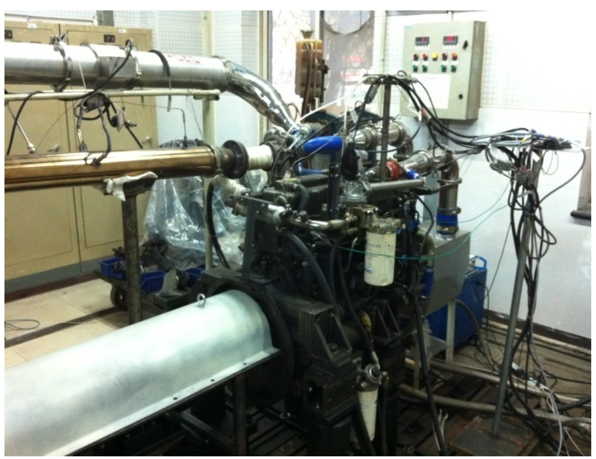
A light-duty diesel engineYC4E170-31 was applied for the experimental evaluation as shown in Figure 10. The control system designed above was implemented on a bypass controller, which communicates with the ECU by the CAN bus. The following experiments are carried out to verify the designed control system.

Figure 10. Test bench of YC4E170-31 diesel engine.

Figure 10. Test bench of YC4E170-31 diesel engine.

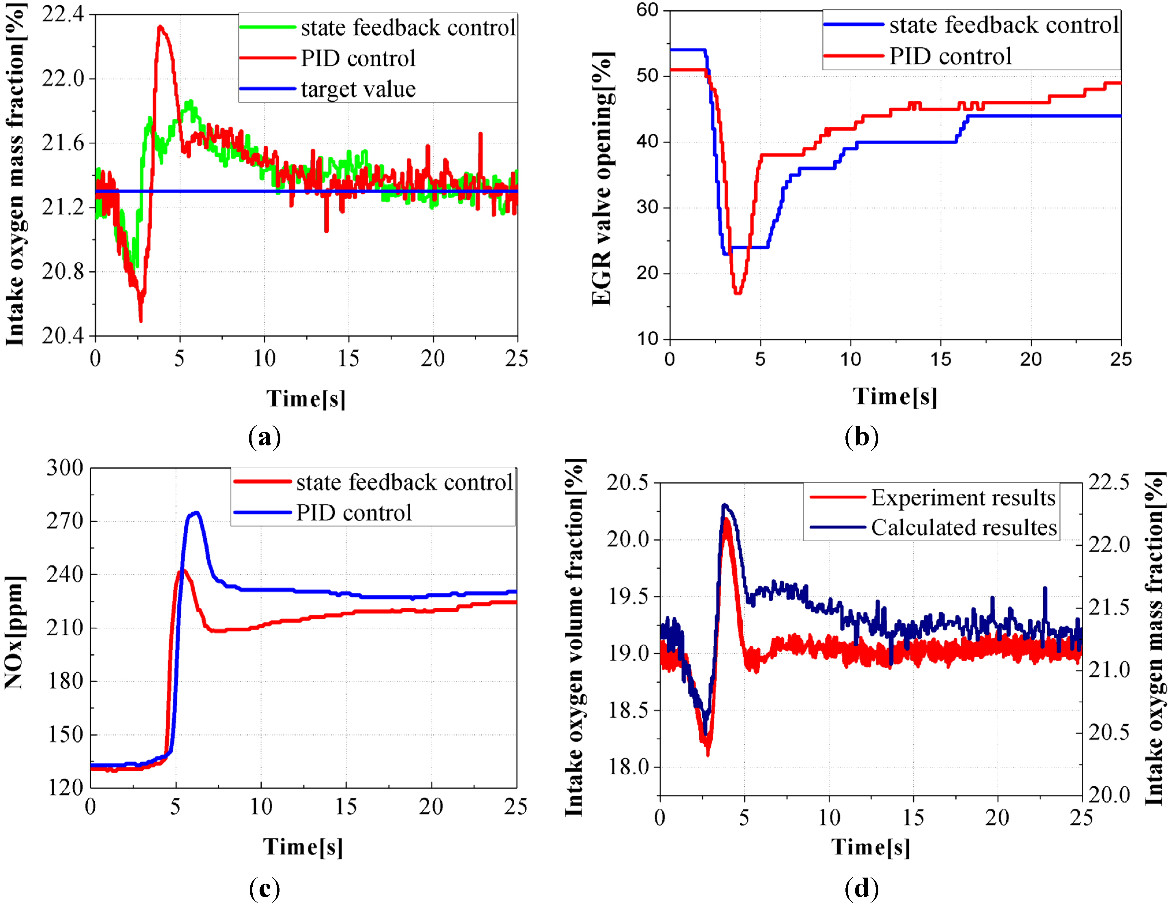
(1) The diesel engine operates at a constant speed of 1500 r/min, the power is increased from 10% to 35% in 1 s, the loading duration time is 3 s. In this process, the control system adjusts the EGR valve opening to maintain a constant intake oxygen mass fraction, with a target of 21.3%. Two different control algorithms, state feedback control and PID control, are applied in the control system, and all the control parameters have been optimized.

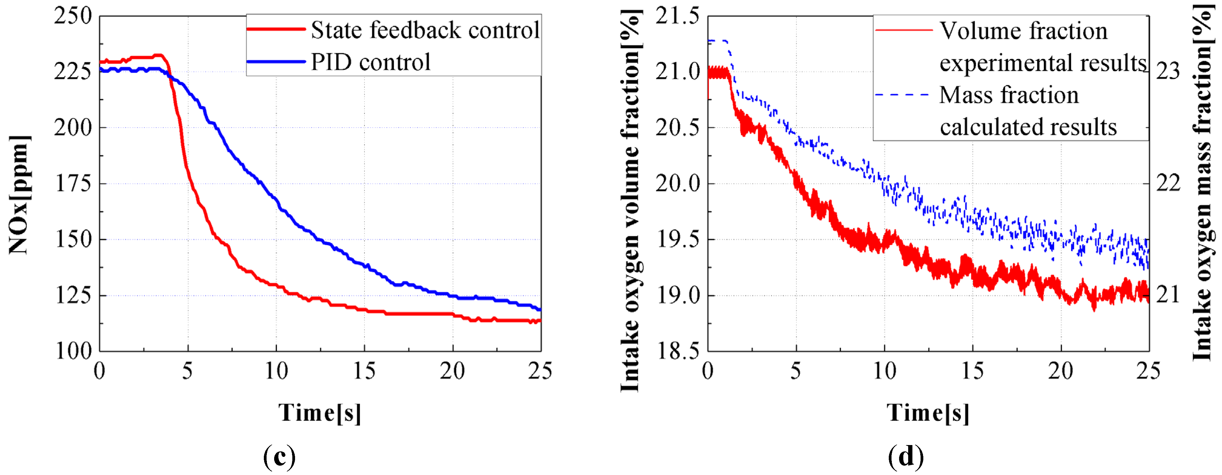
Figure 11 shows the response curves of the two control algorithms. From the changes of the intake oxygen mass fraction and the EGR valve opening, it can be seen that the control precision of the two kinds of control strategies are very similar, but the state feedback controller can provide a faster dynamic response and less overshoot than the PID controller. Figure 11c is the response of the NOx emissions. The NOx emissions under the control of the state feedback controller not only can give a smaller overshoot than under the PID controller, but also result in a lower emission level. Therefore, the state feedback controller is much better than the PID controller in both the control process and the control effect. Figure 11d is the comparison of the calculated intake oxygen mass fraction value and the measured intake oxygen volume fraction value in the PID controller control process. From the figure it can be seen that the two parameters not only have the same change trend, but also have a linear relationship.

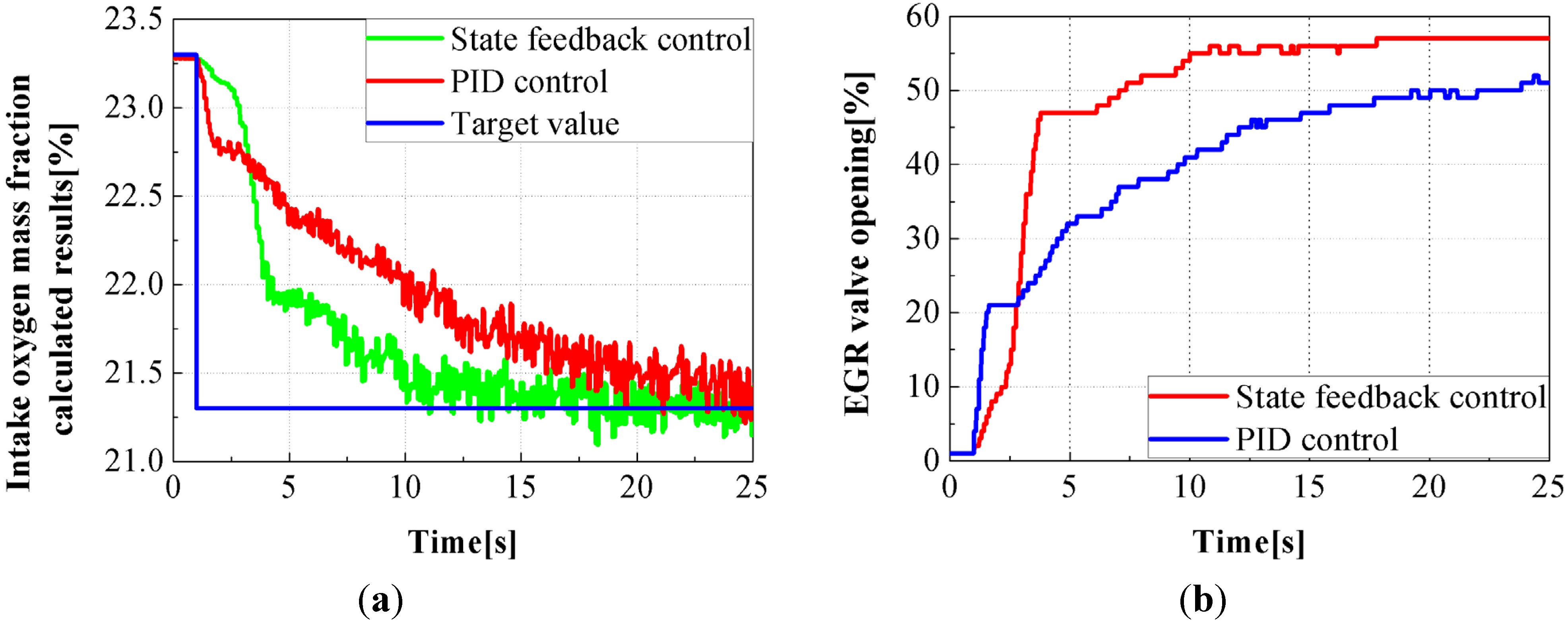
(2) The diesel engine operates at 1500 r/min, 25% load, the target intake oxygen mass fraction has a step change from 23.3% to 21.3% in 1 s. Two different control algorithms, state feedback control and PID control, are used in the control system, in order to contrast the responses of the two control algorithms.

Figure 12 shows the step response of the control algorithm under steady operating conditions. It can be seen from the change trends of the intake oxygen mass fraction and the EGR valve opening that the two algorithms both can achieve accurate tracking of the target value and no overshoot, but the state feedback controller has a shorter adjustment time. The shorter the adjustment time, the quicker the change of the NOx emissions and the lower the NOx emissions in the whole control process. Therefore, the control performance of the state feedback controller is better than the PID controller with the step input. Figure 12d is the curve of the calculated value of the intake oxygen mass fraction and the measurement value of the intake oxygen volume fraction under the adjustment of the PID controller. It shows that the calculated value can accurately track the actual value with the step input.

Figure 11. Comparison of the two kinds of control algorithm under constant speed loading conditions: (a) Intake oxygen mass fraction; (b) EGR valve opening; (c) NOx; (d) intake oxygen volume fraction and intake oxygen mass fraction.

Figure 11. Comparison of the two kinds of control algorithm under constant speed loading conditions: (a) Intake oxygen mass fraction; (b) EGR valve opening; (c) NOx; (d) intake oxygen volume fraction and intake oxygen mass fraction.

Figure 12. Comparison of the two kinds of control algorithm under steady state conditions: (a) Intake oxygen mass fraction calculated results; (b) EGR valve opening; (c) NOx; (d) comparison.

Figure 12. Comparison of the two kinds of control algorithm under steady state conditions: (a) Intake oxygen mass fraction calculated results; (b) EGR valve opening; (c) NOx; (d) comparison.

6. Conclusions and Future Work

In this paper, a novel approach to control a diesel engine EGR system has been proposed. This approach is based on the theory of state feedback control. The state space model was established and validated against a GT-Power model. A state feedback controller based on the intake oxygen mass fraction was designed and the formula of the intake oxygen mass fraction was developed. The designed state feedback controller was validated by the simulation and experimental results. The following conclusions are obtained:

(1)

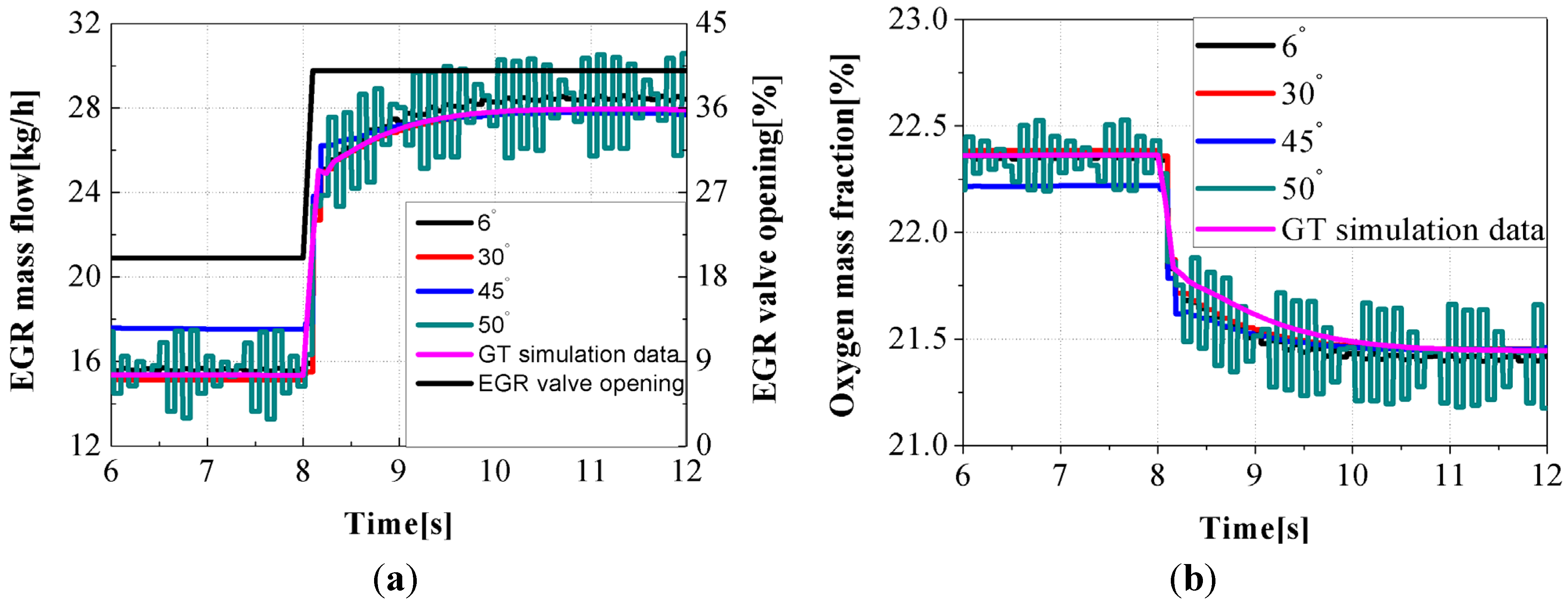
The calculated results of the state space model showed a ±7% difference from the simulation results from the calibrated GT-power model, which means that the designed state space model can accurately describe the dynamic characteristics of the system.

(2)

The intake oxygen mass fraction is a function of EGR rate and the excess air coefficient. This conclusion was verified by the simulation results. The calculated results showed a ±0.5% evaluated error, which means that the estimation method proposed in this paper can be used to accurately estimate the intake oxygen mass fraction.

(3)

It can be seen from the experimental results that compared to the PID controller, the state feedback controller proposed in this paper can achieve a more rapid dynamic response and smaller overshoots in transient control. The designed EGR control system can meet well the control requirements of diesel engine EGR systems in steady and transient conditions.

The state feedback controller of the EGR system has been developed and validated in this paper. Because the state space model is based on a high pressure EGR and fixed geometry turbine, the controller is suitable for turbocharged diesel engines fitted with high pressure EGR systems and fixed geometry turbine, not VGT. In future work, the method described in this paper will be used to design a controller for engines fitted with VGT and/or LP EGR systems. In addition, this controller will be further verified under different operating conditions. The impact of all other variations of operating conditions on the performance of the controller and the control methods will also be investigated in future efforts.

References

1. Lee, S.; Lee, J.; Lee, S.; Kim, D.; Lee, Y.; Yu, S.; Choi, H. Study on Reduction of Diesel Engine Out Emission through Closed Loop Control based on the In-Cylinder Pressure with EGR Model; SAE Technical Paper; SAE International: Warrendale, PA, USA, 2013. [Google Scholar]
2. Chen, S.K.; Yanakiev, O. Transient NOx Emission Reduction Using Exhaust Oxygen Concentration Based Control for a Diesel Engine; SAE Technical Paper 2005-01-0372; SAE International: Warrendale, PA, USA, 2005. [Google Scholar]
3. Reifarth, S.; Angstrom, H.-E. Transient EGR in a High-Speed DI Diesel Engine for a Set of Different EGR-Routings; SAE Technical Paper 2010-01-0372; SAE International: Warrendale, PA, USA, 2010. [Google Scholar]
4. Alberer, D.; del Re, L. Fast Oxygen Based Transient Diesel Engine Operation; SAE Technical Paper 2009-01-0622; SAE International: Warrendale, PA, USA, 2009. [Google Scholar]
5. Ejiri, A.; Sasaki, J.; Kinoshita, Y.; Shimotani, K.; Iizawa, R. Transient control of air intake system in diesel engines. In Proceedings of the SICE Annual Conference, Taipei, Taiwan, 18–21 August 2010; pp. 503–508.
6. Yokomura, H.; Kouketsu, S.; Kotooka, S.; Akao, Y. Transient EGR Control for a Turbocharged Heavy Duty Diesel Engine; SAE Technical Paper 2004-01-0120; SAE International: Warrendale, PA, USA, 2004. [Google Scholar]
7. Ortner, P.; del Re, L. Predictive control of a diesel engine air path. IEEE Trans. Control Syst. Technol. 2007, 15, 449–456. [Google Scholar] [CrossRef]
8. Karlsson, M.; Ekholm, K.; Strandh, F.; Johansson, R.; Tunestal, P. LQG control for minimization of emissions in a diesel engine. In Proceedings of the IEEE International Conference on Control Applications, San Antonio, TX, USA, 3–5 September 2008; pp. 245–250.
9. Utkin, V.I.; Chang, H.-C.; Kolmanovsky, I.; Cook, J.A. Sliding mode control for variable geometry turbocharged diesel engines. In Proceedings of the American Control Conference, Chicago, IL, USA, 28–30 June 2000; pp. 584–588.
10. Dorf, R.C.; Bishop, R.H. Modern Control Systems; Pearson: London, UK, 2011. [Google Scholar]
11. Ammann, M.; Fekete, N.; Guzzella, L.; Glattfelder, A.H. Model-Based Control of the VGT and EGR in a Turbocharged Common-Rail Diesel Engine Theory and Passenger Car Implementation; SAE Technical Paper Series 2003-01-0357; SAE International: Warrendale, PA, USA, 2003. [Google Scholar]
12. Ouenou-Gamo, S.; Rachid, A.; Ouladsine, M. A nonlinear controller of a turbocharged diesel engine using sliding mode. In Proceedings of the 1997 IEEE International Conference on Control Applications, Hartford, CT, USA, 5–7 October 1997; pp. 803–805.
13. Hopka, M.; Upadhyay, D.; Guezennec, Y.; Rizzoni, G. Identification of a mean value model of a modern diesel engine for control design. In Proceedings of the ASME 2003 International Mechanical Engineering Congress and Exposition, Washington, DC, USA, 15–21 November 2003; pp. 1069–1077.
14. Fredriksson, J.; Egardt, B. Estimating exhaust manifold pressure in a turbocharged diesel engine. In Proceedings of the 2002 International Conference on Control Applications, Glasgow, UK, 18–20 September 2002; pp. 701–706.
15. Guzzella, L.; Onder, C.H. Introduction to Modeling and Control of Internal Combustion Engine Systems; Springer: Berlin, Germany, 2004. [Google Scholar]
16. Jung, M.; Ford, R.G.; Glover, K.; Collings, N.; Christen, U.; Watts, M.J. Parameterization and Transient Validation of a Variable Geometry Turbocharger for Mean-Value Modeling at Low and Medium Speed-Load Points; SAE Technical Paper 2002-01-2729; SAE International: Warrendale, PA, USA, 2002. [Google Scholar]
17. Storset, O.F.; Stefanopoulou, A.G.; Smith, R. Adaptive air charge estimation for turbocharged diesel engines without exhaust gas recirculation. J. Dyn. Syst. Meas. Control 2004, 126, 633–643. [Google Scholar] [CrossRef]
18. Storset, O.F.; Stefanopoulou, A.; Smith, R. Air charge estimation for turbocharged diesel engines. In Proceedings of the American Control Conference, Chicago, IL, USA, 28–30 June 2000; pp. 39–44.
19. Xiaohui, A.; Bolan, L.; Fujun, Z.; Geng, F. Simulation of the effect of intake charge oxygen concentration based EGR on diesel engine performance. Trans. CSICE 2013, 31, 115–119. [Google Scholar]
20. Chauvin, J.; Corde, G.; Petit, N. Transient control of a Diesel engine airpath. In Proceedings of the ACC’07 American Control Conference, New York, NY, USA, 9–13 July 2007; pp. 4394–4400.
21. Marino, R.; Tomei, P. Nonlinear Control Design: Geometric, Adaptive and Robust; Prentice Hall International (UK) Ltd.: Hertfordshire, UK, 1996. [Google Scholar]
22. Kirk, D.E. Optimal Control Theory: An Introduction; Courier Dover Publications: Mineola, NY, USA, 2012. [Google Scholar]
23. Ogata, K. Modern Control Engineering; Pearson Education: New York, NY, USA, 2010. [Google Scholar]