The Optimum PV Plant for a Given Solar DC/AC Converter

Abstract

In recent years, energy production by renewable sources is becoming very important, and photovoltaic (PV) energy has became one of the main renewable sources that is widely available and easily exploitable. In this context, it is necessary to find correct tools to optimize the energy production by PV plants. In this paper, by analyzing available solar irradiance data, an analytical expression for annual DC power production for some selected places is introduced. A general efficiency curve is extracted for different solar inverter types, and by applying approximated function, a new analytical method is proposed to estimate the optimal size of a grid-connected PV plant linked up to a specific inverter from the energetic point of view. An exploitable energy objective function is derived, and several simulations for different locations have been provided. The derived analytical expression contains only the available data of the inverter (such as efficiency, nominal power, etc.) and the PV plant characteristics (such as location and PV nominal power).

1. Introduction

Renewable energy sources have become the most prevalent energy sources in recent years, and researchers have made considerable effort to enhance the efficiency of these systems and to optimize the functionality.

Grid-connected photovoltaic (PV) systems grew up very fast in the last few decades; however the energy production by PV systems is still too expensive when compared with other conventional technologies. Moreover, it should be noted that many countries implement policies of economic incentives to encourage the production of electricity from renewable sources, and in particular, the solar one is still financed in a consistent manner. In most cases, these incentives are designed in order to be more and more advantageous with the increasing energy production by the PV plants.

A grid-connected PV system consists of PV arrays, an inverter to convert the produced DC to AC power and, in most cases, a transformer to couple the system to the network [1].

A way to reduce the cost impact of this technology is to select each part of a PV plant with respect to achieving the maximum energy and economic performance [2,3,4,5,6,7,8]. For this purpose, the inverter rated capacity (P_nINV) must be matched with the rated PV array capacity (P_PVpeak) to reach the optimum PV system performance [9].

On the other hand, the optimal P_PVpeak/P_nINV sizing ratio depends on the local climate, the PV surface orientation and inclination, the inverter performance and the PV/inverter cost ratio [9].

Conventionally, the rated power of a DC/AC inverter is selected as equal to the total nominal power of the installed PV array. This solution often does not match the requirement of the optimum functioning of the systems: first, although the nominal power of the PV array is calculated under the standard test condition (STC), the statistics show that STC irradiance occurs very rarely; second, there are other factors affecting the PV system performance, such as ambient temperature, wind blowing, tilt angle, and so on. In addition, sunshine and high irradiance do not necessarily lead to a high power output. For most places, more sunlight exposure usually implies a hot climate: this high correlation between irradiance level and temperature results in a counteraction between these two factors and deteriorates the performances of both the PV array and inverter. In this case, the exact optimum inverter size is not determined; therefore, a more in-depth analysis is required [10].

Under-sizing the DC/AC inverter regarding the nominal PV array is often a suggested solution to enhance the performance and decrease the costs of the whole system; however, there is not a common definition that can be adopted for all locations in order to calculate the precise ratio between inverter and PV plant rated power.

In [11], it is reported that in Central Europe, the optimum performance of a grid-connected PV system can be achieved for an inverter size of 0.6–0.7-times the PV rated capacity. This means that the P_PVpeak/P_nINV ratio varies between 1.43 and 1.67. Kil and Van der Weiden in [12] found that PV system performance remained unaffected when the inverter/PV rated power ratio was 0.67 (P_PVpeak/P_nINV = 1.49) in Portugal and 0.65 (P_PVpeak/P_nINV = 1.54) in the Netherlands. In [13], Burger and Ruther have shown that this practice might lead to considerable energy losses, especially in the case of PV technologies with high temperature coefficients of power operating in cold climate sites and also with low temperature coefficients of power operating in warm climate sites (which means that the energy distribution of sunlight is shifted to higher irradiation levels).

The optimum inverter sizing ratio in Madrid (40.5N) and Trappes (48.7N) was reported as 1.25 (P_PVpeak/P_nINV = 0.80) and 1.42 (P_PVpeak/P_nINV = 0.70), respectively [14]. In [15] it was shown that the inverter/PV rated power ratio in Kassel, Germany, is 0.75 (P_PVpeak/P_nINV = 1.33) and 1.0 for Cairo, Egypt. In addition, it was found in [16] that the optimum sizing ratio (P_PVpeak/P_nINV) varied from 1–2 for different locations and conditions. Overall, both under-sizing and over-sizing are suggested for different considerations.

In [1], an analytical method is presented to find the optimized size of the inverter. It considers the maximum available DC power as a variable and tries to find the optimum inverter size for a specific PV system. Since it deals with an installed PV array as the input, the results for the inverter size are around the available DC maximum power, and it suggests an inverter size slightly higher than the maximum available DC power.

There are several other methods for sizing solar power plants in terms of the optimum ratio between the nominal PV array capacity and the rated inverter input capacity leading to discordant conclusions [8,15,16,17,18,19,20]. Even if these practices lead to PV systems that work without any problems, these solutions are not often the optimum from the energy point of view. Indeed, one key element in the energy optimization is the correct selection of the right profile concerning the energy production of the PV array with respect to the nominal power of the DC/AC inverter. It is very important, therefore, to find an adequate function that is able to consider all of the elements in order to find the optimum rated PV plant depending on the power of the inverter.

Instead, if we consider all of the different types of inverters, each with its specific performance, it is not possible to find the optimal one for a specific PV plant in a specific location. On the other side, it is possible to find an optimal PV plant for a given inverter in a specific location, since the production of the PV plant is proportional to its size (kW) only.

This paper, contradictory to [1], tries to find the optimal PV array power rating in a specific location considering a specified DC/AC inverter. Therefore contradictory to the literature, the goal is to set up an analytical method in order to define the optimal PV plant size in a specific location. The proposed method put in evidence that a very important factor for the optimization is the power duration curve. Consequently, the proposed method will be based on the hourly average irradiation curve and the approximated efficiency curve of the inverter [21].

This paper discusses the analysis and the procedure based on extracted data from PVsyst software. Hence, available data are used as a good example to illustrate the method, and the reliability of these data is not our concern.

2. Solar Irradiance and DC Power at the Output of PV Modules

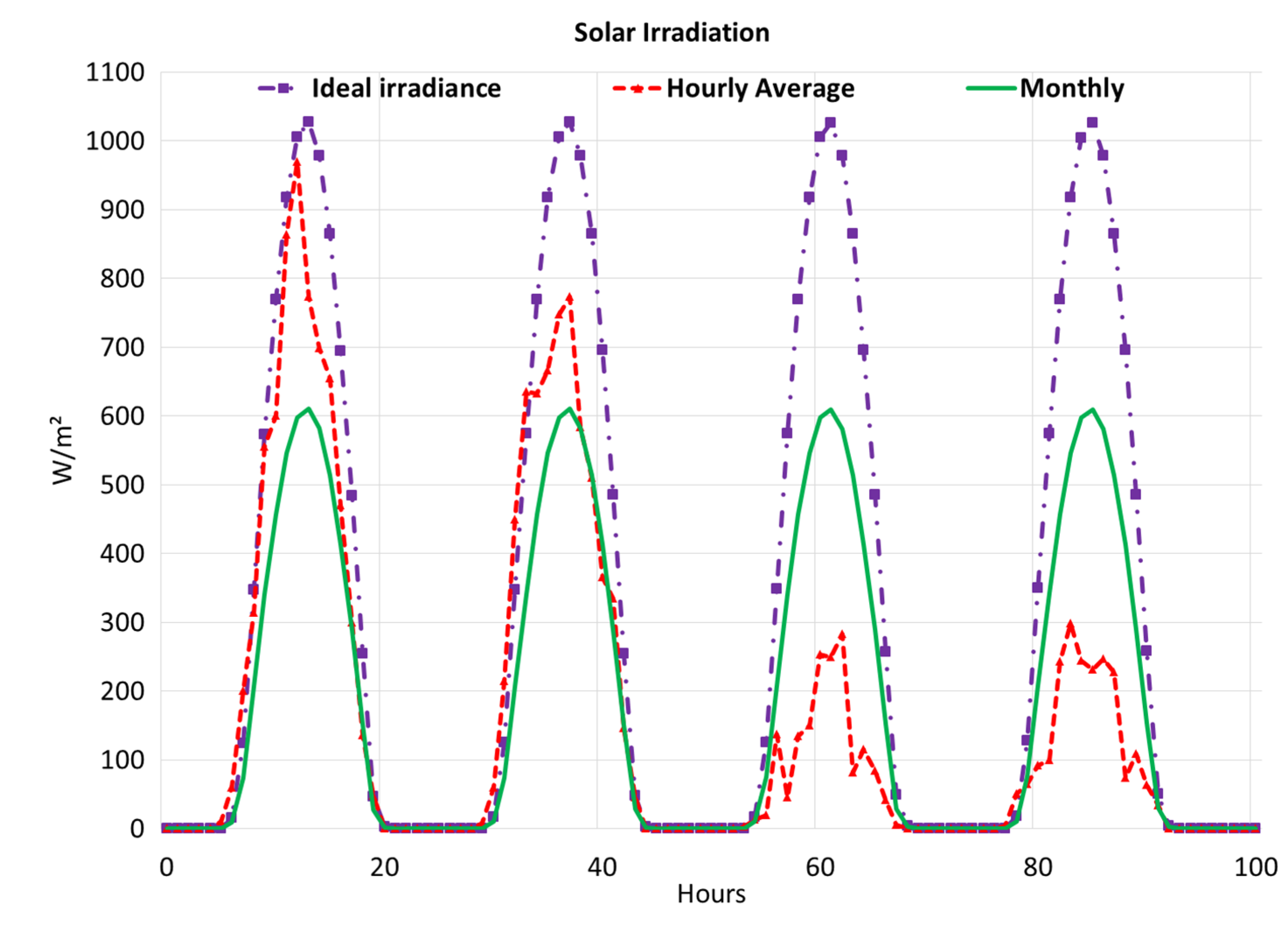
The first parameters to be considered are the solar irradiance and the ambient temperature. These depend on the geographic location, on the time of the day and on the day of the year. Figure 1 shows the ideal irradiation curve (with clear sky) in comparison with the monthly and the hourly average curves in a PV system with a fixed tilted surface facing south (azimuth = 0°).

Adverse weather and other environmental conditions (such as pollution, clouds, shadows, and so on) affect the actual solar irradiance greatly at the ground level, which leads more often to a lower amplitude of the average curve compared to the ideal one, as is shown in Figure 1. Therefore, the trend of the actual solar irradiance over the daytime cannot be approximated by a Gaussian curve, as proposed in many papers, because the actual curve is very different. Besides, even the ambient temperature affects the PV production, owing to the PV panel current/voltage (I-V) curve depending on the solar irradiance and the cell temperature.

Starting with the I-V curve of the module, since the solar irradiance and the relative cell temperature values are known, the power-voltage (P-V) curve can be calculated. Moreover, the maximum DC power extraction is considered, so the DC/AC converter needs to impose on the PV panels the appropriate voltage. It can be assumed that the PV panel always operates at its maximum power point (MPP) for any given solar irradiance and cell temperature. Several average values of solar irradiance and cell temperature with different time resolutions (15 min, 1 h and one day) are available in the literature, and all of these data are excellent for making simulations for evaluating the yearly PV plant energy production, but they are useful for the optimization of the DC/AC converter sizing only if the time resolution is not too big. For instance, from Figure 1, monthly average representation is too smooth and far from reality.

Figure 1. Example of the comparison between ideal, monthly and hourly average solar irradiance values (Paris: azimuth 0°; tilt 32°).

Figure 1. Example of the comparison between ideal, monthly and hourly average solar irradiance values (Paris: azimuth 0°; tilt 32°).

The electric power at the DC terminals of a PV array, P_DC(t), is directly proportional to the solar irradiance and varies linearly with the solar cell temperature. It is expressed as:

$$P_{DC}\left(t\right)=P_{PVpeak}\cdot \frac{I\left(t\right)}{I_{STC}}\cdot \left[1-DP\cdot \Delta \vartheta \right]$$

(1)

where:

-

P_DC(t) is the duration curve, defined as the curve that shows the cumulative time in a year during which the DC power is larger or equal to a certain value; therefore, it is the available DC power at time t, in kW;

-

P_PVpeak is the installed peak power of all the PV modules under standard test conditions (STC), in kW;

-

I(t) is the solar irradiance at time t, in W/m²;

-

I_STC, equal to 1000 W/m², is the solar irradiance under STC;

-

DP is a coefficient that expresses the power variation due to the temperature rise of the cells. A typical value of DP, for crystalline silicon cells, is −0.5%/°C;

-

Δϑ, in °C, is the rise of the temperature of the cell above 25 °C.

Usually, the cell temperature rises 30 °C above the ambient temperature when electric current flows through the cell. Thus, Δϑ can be approximately calculated from the ambient temperature, T_amb, using:

Δϑ = T_amb + 30 °C − 25 °C

(2)

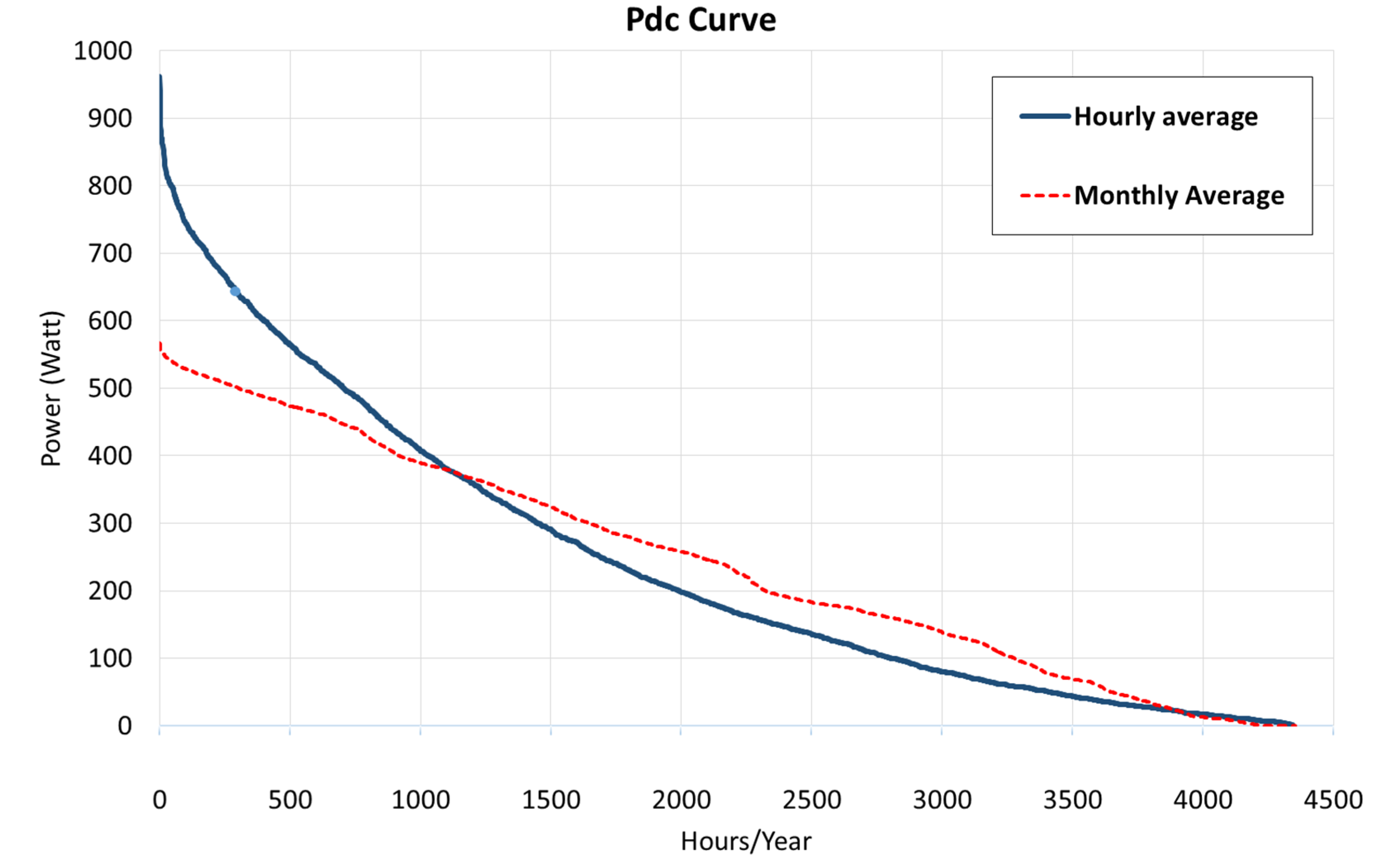
The DC power, P_DC(t), of one PV installation with P_PVpeak nominal power has been calculated with 1-h and with one-month resolution using the solar irradiance and ambient temperature data available in the literature. The result is shown in Figure 2.

Figure 2. P_DC duration curves, calculated from monthly and hourly average solar irradiance values (Paris: azimuth 0°; tilt 32°).

Figure 2. P_DC duration curves, calculated from monthly and hourly average solar irradiance values (Paris: azimuth 0°; tilt 32°).

With reference to Figure 2, there is a big difference between the two annual P_DC curves, coming from the hourly and the monthly average irradiation, of the same PV plant with the same nominal power and ambient temperature. The hourly average irradiation represents much better what happens in reality. In the case of the hourly curve, the maximum power of the DC power duration is higher than the monthly average curve. Besides, the shape of the two curves is very different, because the hourly average duration curve can be approximated by a parabolic function, whereas the monthly average curve by a straight line.

Even if the representation does not influence the evaluation of the yearly energy production of the PV plant, it is easy to understand that the time resolution is a very important factor in inverter sizing, as reported in [13]. Therefore, monthly, daily, hourly and shorter interval (e.g., every minute or 10 s) time representation can affect the inverter sizing strongly. For instance, monthly time resolutions, which has been widely used in the literature, are too far from reality to calculate peak spots of solar irradiance, and therefore, the results are not correct. Based on this fact, the use of the monthly average P_DC curve can lead to under-sizing the inverter and considerable power losses [13]. For this reason, in this paper, the authors have adopted the hourly P_DC curve to find the optimum solution.

3. Annual P_DC Analytical Representation

The P_DC curves can be approximated by the following analytical expression:

$${\dot{p}}_{dc}\left(\dot{t}\right)=\mathrm{\alpha }\cdot {\dot{t}}^2+\mathrm{\beta }\cdot \dot{t}+\gamma$$

(3)

where α, β and γ are the coefficients to be determined,

$${\dot{p}}_{dc}\left(\dot{t}\right)=\frac{P_{DC}(t)}{P_{PVpeak}}$$

and:

$$\dot{t}=\frac{t}{T_{\max \_PV}}$$

where ${\dot{p}}_{dc}\left(\dot{t}\right)$ and $\dot{t}$ stand for respective per-unit values of power and time; in particular, P_PVpeak is the available peak PV power and T_{max_PV} is the maximum time during one year when solar energy is available at the site; therefore:

$$P_{DC}(t)=\frac{P_{PVpeak}}{T_{\max \_PV}^2}\cdot \mathrm{\alpha }\cdot t^2+\frac{P_{PVpeak}}{T_{\max \_PV}}\cdot \mathrm{\beta }\cdot t+\gamma \cdot P_{PVpeak}$$

(4)

It is important to underline that the maximum annual duration of the DC power, T_{max_PV}, is approximately the same for every location. This is due to the natural rotation of the Earth around its axis and to the Sun. Assuming that T_{max_PV} is constant for every location and equal to 4350 h, less than a 0.6% error is inserted. The small differences in T_{max_PV} between the locations are due to the tilt of the Earth’s axis, which makes the Northern Hemisphere receive sunlight for longer periods during a year than the southern one.

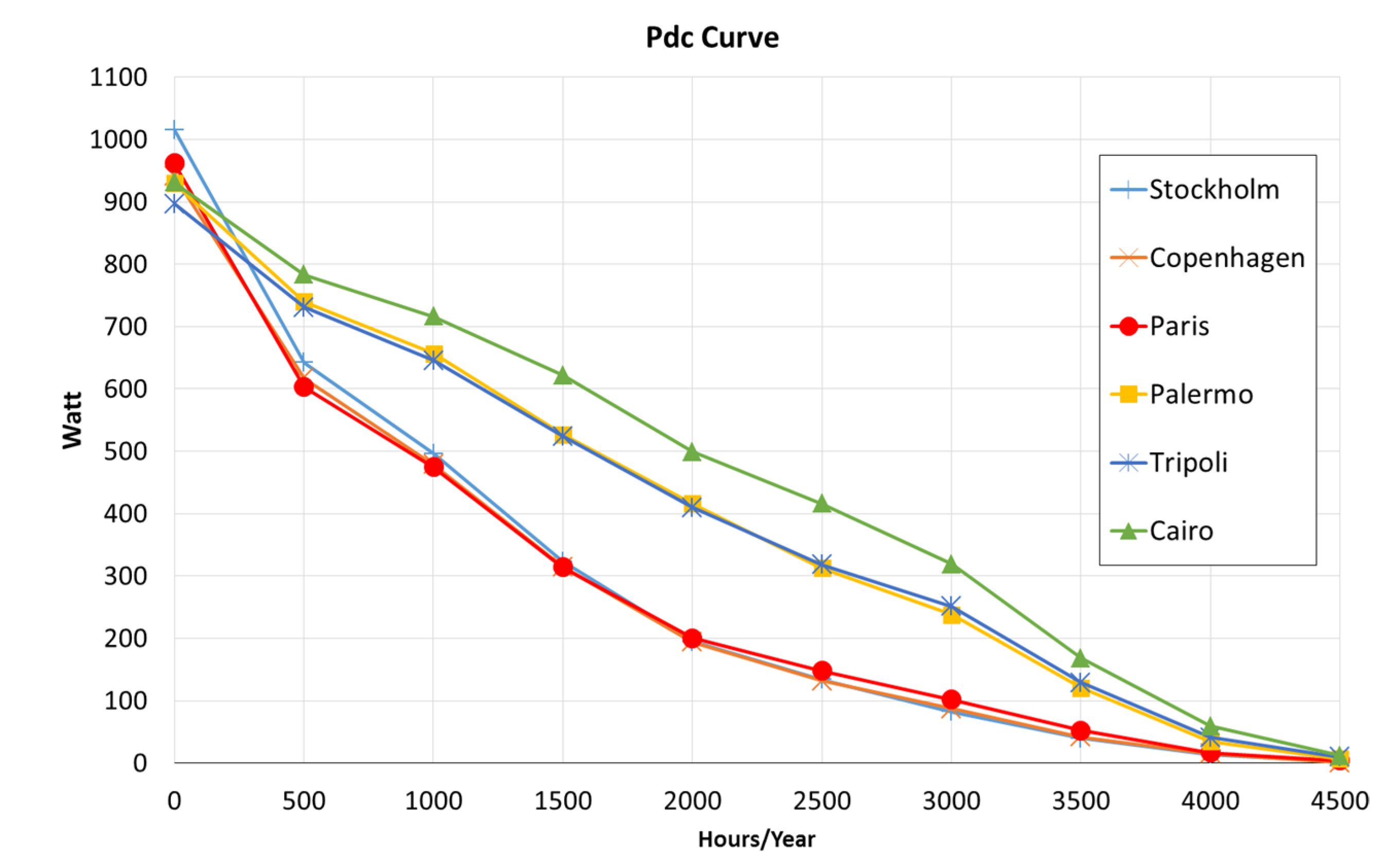
Figure 3 shows the P_DC duration curves evaluated for some locations, at the optimum tilt angle. Table 1 shows the parabolic and correlation coefficients of the P_DC duration curves. In order to find the coefficients and correlations, here, “Trendline” options of Microsoft Excel software have been used.

Figure 3. Duration curves of 1 kilowatts peak (kWp) PV plants located in different cities with their optimal modules’ tilt.

Figure 3. Duration curves of 1 kilowatts peak (kWp) PV plants located in different cities with their optimal modules’ tilt.

Table 1. Coefficients of 1-kWp PV power plants in some cities by real irradiance simulated with PVsyst software. Dbase Meteonorm ’97.

Location	Stockholm	Copenhagen	Paris	Palermo	Tripoli	Cairo
Latitude	59.1° N	55.4° N	49.1° N	38.0° N	32.8° N	30.1° N
Tilt (optimum) (angle°)	41	38	35	32	29	26
PDCmax (W)	1016	942	962	930	897	931
Tmax_PV (h)	4323	4305	4346	4339	4358	4354
α	1.0243	0.9459	0.8829	0.1900	0.18115	−0.1433
β	−1.7946	−1.6815	−1.5979	−1.0585	−1.0261	−0.7511
γ	0.8052	0.7690	0.7487	0.8433	0.8300	0.8638
R2 (%)	0.99610	0.9948	0.9934	0.9976	0.9989	0.9979

Table 1. Coefficients of 1-kWp PV power plants in some cities by real irradiance simulated with PVsyst software. Dbase Meteonorm ’97.

Location	Stockholm	Copenhagen	Paris	Palermo	Tripoli	Cairo
Latitude	59.1° N	55.4° N	49.1° N	38.0° N	32.8° N	30.1° N
Tilt (optimum) (angle°)	41	38	35	32	29	26
PDCmax (W)	1016	942	962	930	897	931
Tmax_PV (h)	4323	4305	4346	4339	4358	4354
α	1.0243	0.9459	0.8829	0.1900	0.18115	−0.1433
β	−1.7946	−1.6815	−1.5979	−1.0585	−1.0261	−0.7511
γ	0.8052	0.7690	0.7487	0.8433	0.8300	0.8638
R2 (%)	0.99610	0.9948	0.9934	0.9976	0.9989	0.9979

As regards the studied cases, the correlation coefficient range varies from 99.34% (for Paris with tilt equal to 35°) to 99.89% (for Tripoli, with tilt equal to 29°). Considering coefficients α, β and γ from Table 1, it can be noticed that the P_DC curves are very similar for locations with high optimum tilt values, while at the lower tilts (such as Cairo), the parabolic approximation is different. Another feature is that all of the curves begin approximately from the same point, indicating that, as expected, the peak value is almost equal in each location.

Although Equation (3) can be valid for every location and for PV panels with crystalline silicon cells, it involves some inaccuracies that should be mentioned:

• In Equation (1), it is assumed that the P_DC is directly proportional to the solar irradiance, which means that the efficiency of the PV panels is constant and does not depend on the level of solar irradiance. In reality, the conversion efficiency of a PV panel drops slightly as the incident to its surface solar irradiance drops. For example, the efficiency of a typical PV panel with mono-crystalline silicon cells drops from 13.2% at 1000 W/m² to 12% at 200 W/m², so the inserted error is around 1%;
• In Equation (2), it is assumed that the increase in the cell temperature is 30 °C independent of the power level at which it is working. The increase in temperature is in the range 22–37 °C depending on the ambient temperature, the wind speed and the level of irradiance, which varies in a stochastic way. Hence, the 30 °C increase in temperature used in (2) is a mean value. Moreover, the maximum error introduced in the P_DC(t) calculation, when assuming a 30 °C temperature rise instead of 22 °C or 37 °C, depends on the ambient temperature. For T_amb = 20 °C, the respective errors are 4.4% and 4.1%. It should be mentioned, however, that this error is not due to the specific method followed in this paper, but it is added in all of the calculation methods followed in literature.

Since the respective error by both above-mentioned inaccuracies is less than 5%, these do not affect significantly the shape of the P_DC(t) curve.

In conclusion, it is important to underline that the P_DC duration curve of any PV installation in any location can be represented as a parabolic curve, although in some cases, it can be a linear one.

4. The Efficiency Curve of a PV Inverter

Solar inverters are complex power electronic devices comprising often a DC/DC boost converter to boost up the PV array DC output voltage and to guarantee the MPPT working principle [20,22] and a DC/AC inverter, which is controlled as the current source to produce the output AC power in the unity power factor. This device is the interface between DC side and the AC grid. The efficiency η of a given solar inverter is defined by:

$$\mathrm{\eta }\text{\hspace{0.17em}}=\frac{P_{AC}\left(t\right)}{P_{DC}\left(t\right)}=\frac{P_{DC}\left(t\right)-P_{loss}\left(t\right)}{P_{DC}\left(t\right)}=1-\frac{P_{loss}\left(t\right)}{P_{DC}\left(t\right)}$$

(5)

where P_DC(t), P_AC(t) and P_loss(t) are the instantaneous DC power, AC power and power losses, respectively.

The power losses of such device consist of two distinct parts. The first is constant and involves the power to supply the control unit and the other auxiliary parts only, while the second is load dependent and consists of: switching losses on power switches, ohmic losses and the losses caused by temperature variation. Therefore, the total loss of the inverter is not constant, and the efficiency is mainly load current dependent.

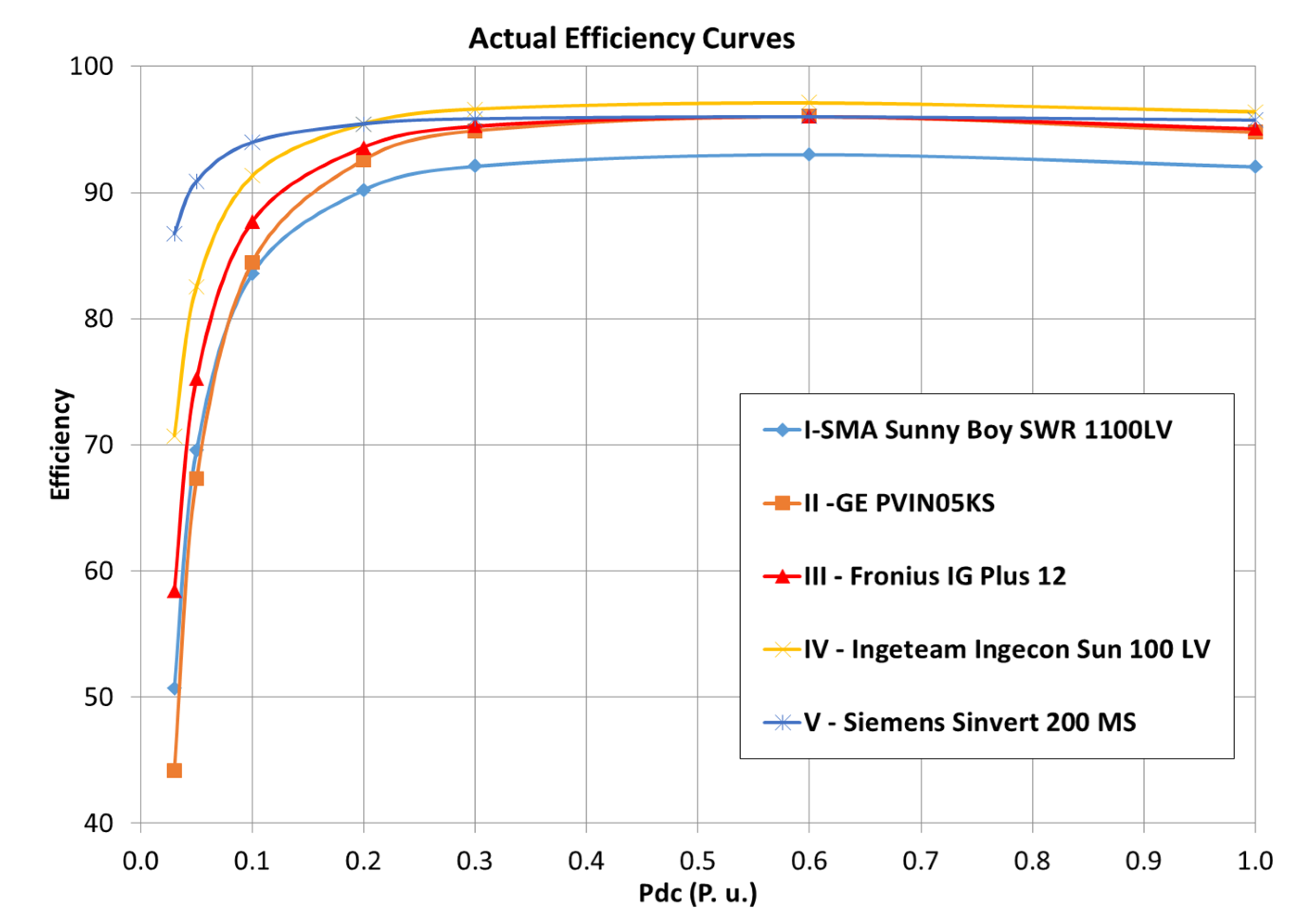
Examples of variation of the efficiency of some inverters are shown in Figure 4, according to the data provided by the manufacturers in the respective technical brochures. It is evident that the conversion efficiency of a solar inverter is a load function. In PV plants, the inverter will work in every possible power level; hence, to evaluate its efficiency over the whole operating range, it is necessary to determine the working range of the PV plant.

Figure 4. Typical per unit efficiency curves for grid-connected solar inverters.

Figure 4. Typical per unit efficiency curves for grid-connected solar inverters.

The following simple mathematical function describes, with very good accuracy for loads >2%, the efficiency curve of any solar inverter [1]. By imposing:

$${\dot{p}}_{INV\_DC}\left(\dot{t}\right)=\frac{P_{INV\_DC}\left(t\right)}{P_{nINV\_DC}}$$

where P_{nINV_DC} is the nominal DC power of the inverter and P_{INV_DC} is inverter DC power, we can have:

$$\mathrm{\eta }\left({\dot{p}}_{INV\_DC}\right)=A+B\cdot {\dot{p}}_{INV\_DC}\left(t\right)+\frac{C}{{\dot{p}}_{INV\_DC}\left(t\right)}$$

(6)

where $\mathrm{\eta }\left({\dot{p}}_{INV\_DC}\right)$ is the efficiency of the inverter as a percentage, ${\dot{p}}_{INV\_DC}\left(t\right)>0$ is the per unit (p.u.). value of the DC power that the inverter can convert in AC, while A, B and C are some parameters that should be determined.

It is obvious from (6) that three pairs of [$\mathrm{\eta }\left({\dot{p}}_{INV\_DC}\right)$, ${\dot{p}}_{INV\_DC}\left(t\right)$] values are needed to determine the A, B and C parameters. These pairs are readily available from the inverter efficiency curve provided by the manufacturers. A very good choice are the pairs corresponding to:

-

the central point of the curve angle ${\dot{p}}_{INV\_DC}=0.1$;

-

the end of the curve angle ${\dot{p}}_{INV\_DC}=0.2$;

-

the final point of the curve ${\dot{p}}_{INV\_DC}=1.0$.

It is important to underline that these values are available in the data sheets of the manufacturers. Therefore, the efficiency curve defined by the parameters A, B and C can now be easily calculated by solving the following system:

$$\{\begin{array}{l}{\mathrm{\eta }}_{10\%}=A+0.1\cdot B+10\cdot C\\ {\mathrm{\eta }}_{20\%}=A+0.2\cdot B+5\cdot C\\ {\mathrm{\eta }}_{100\%}=A+B+C\end{array}$$

(7)

Equation (6) describes accurately the efficiency curve of any inverter, and the A, B and C parameters are estimated by the simple system of linear equations reported in Equation (7). It should also be noted that in the solar inverters considered, we have always A > 0, while B and C are less than zero, but those values differ. Hereunder, in Table 2, some different manufacturers’ specifications, shown in Figure 4 and found in the commercial PVsyst inverter database, have been used to calculate the A, B, C and R² coefficients.

Table 2. Some inverter specifications found in the commercial PVsyst database and A, B, C and R² coefficients calculated for the same inverters.

Type	PnINV (kW)		η MAX	A	B	C	R2
	AC	DC
I	1	1.1	93.0	98.236	−4.786	−1.42	0.998
II	5	-	96.0	102.53	−6.019	−1.75	1.000
III	12	12.6	96.0	100.83	−4.517	−1.27	1.000
IV	100	105	97.1	100.56	−3.283	−0.89	0.998
V	200	210	96.0	97.24	−1.194	−0.31	0.995

Table 2. Some inverter specifications found in the commercial PVsyst database and A, B, C and R² coefficients calculated for the same inverters.

Type	PnINV (kW)		η MAX	A	B	C	R2
	AC	DC
I	1	1.1	93.0	98.236	−4.786	−1.42	0.998
II	5	-	96.0	102.53	−6.019	−1.75	1.000
III	12	12.6	96.0	100.83	−4.517	−1.27	1.000
IV	100	105	97.1	100.56	−3.283	−0.89	0.998
V	200	210	96.0	97.24	−1.194	−0.31	0.995

Therefore, the efficiency curve of any inverter can be accurately described by a simple mathematical expression with three unknown parameters, which can be estimated from the data provided by the inverter manufacturer, by simply solving a system of three linear equations.

5. The Optimum PV Plant for a Specific Inverter: Parameter Evaluation

This section deals with an analytical approach to derive the parametric equation of converted energy at the AC side of a solar inverter. In order to evaluate the optimum PV plant for a specific inverter, it is useful to change (3) in the following way:

$${\underset{¯}{\dot{p}}}_{dc}\left(\dot{t}\right)=\frac{P_{DC}(t)}{P_{nINV\_DC}}=\frac{P_{PVpeak}}{P_{nINV\_DC}\cdot T_{\max \_PV}^2}\mathrm{\alpha }\cdot t^2+\frac{P_{PVpeak}}{P_{nINV\_DC}\cdot T_{\max \_PV}}\mathrm{\beta }\cdot t+\gamma \cdot \frac{P_{PVpeak}}{P_{nINV\_DC}}$$

Now, the ${\underset{¯}{\dot{p}}}_{dc}\left(\dot{t}\right)$ is the power energy in the DC side normalized in P_{nINV_DC}. Then, it is possible to write:

$${\underset{¯}{\dot{p}}}_{dc}\left(\dot{t}\right)={\mathrm{\alpha }}^1\cdot t^2+{\mathrm{\beta }}^1\cdot t+{\gamma }^1$$

(8)

where:

$${\mathrm{\alpha }}^1=\mathrm{\alpha }\cdot \frac{P_{PVpeak}}{P_{nINV\_DC}\cdot T_{\max \_PV}^2},{\mathrm{\beta }}^1=\mathrm{\beta }\cdot \frac{P_{PVpeak}}{P_{nINV\_DC}\cdot T_{\max \_PV}} \text{and} {\gamma }^1=\gamma \cdot \frac{P_{PVpeak}}{P_{nINV\_DC}}$$

To find the optimum PV plant for a given inverter, it is necessary to combine Equations (6) and (8). Doing so, it is possible to study two distinctive cases:

In the first case (Case A), P_{nINV_DC} ≥ P_DCmax; therefore, it is assumed that the nominal DC power of the inverter, P_{nINV_DC}, is larger than the P_DCmax, which is the maximum available DC power of the PV plant (equal to P_PVpeak at the standard test conditions).

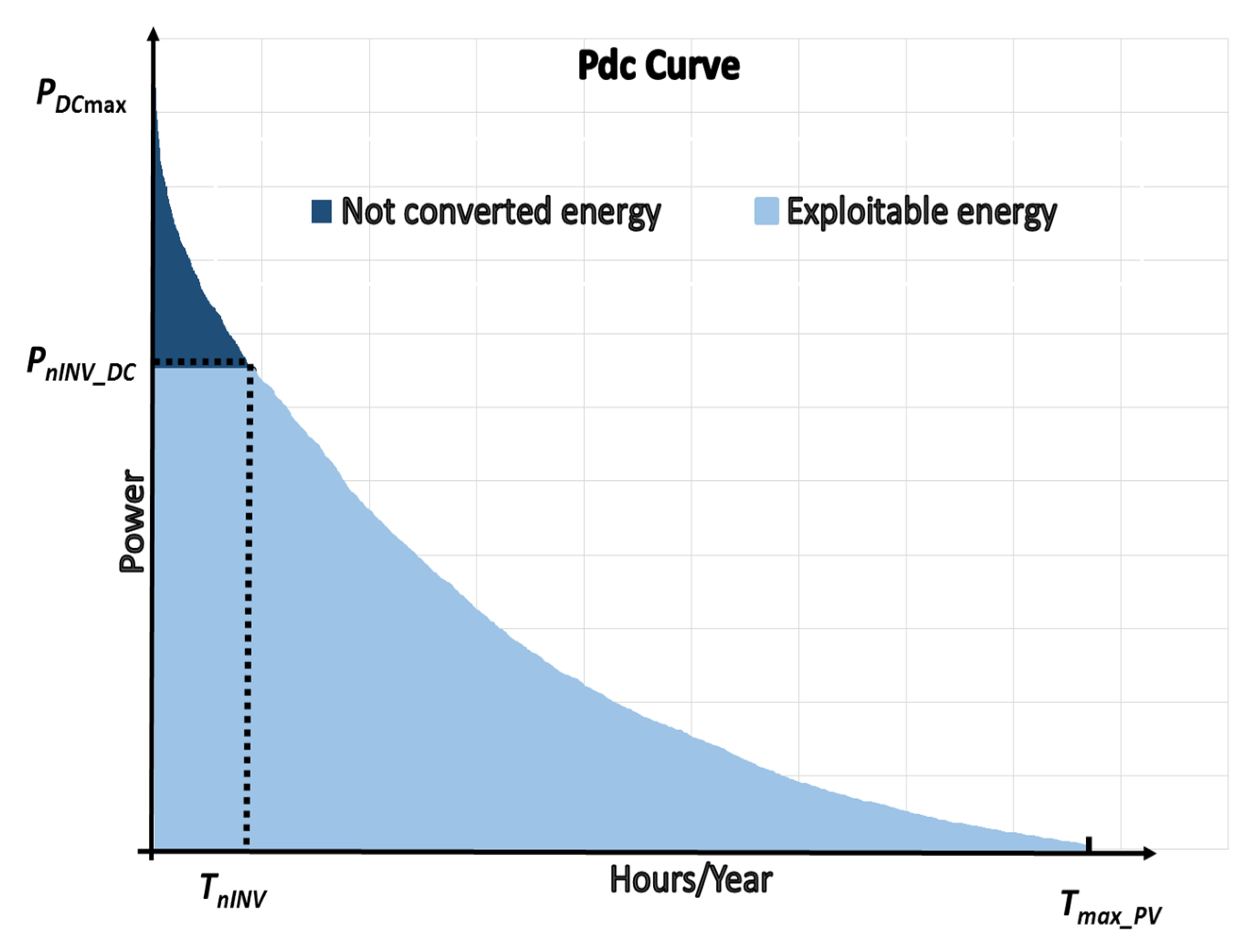
In the second case (Case B), P_{nINV_DC} < P_DCmax; it is assumed that the nominal DC power of the inverter, P_{nINV_DC}, is lower than P_DCmax. As shown in Figure 5, in Case B, the inverter will operate for T_nINV h/year, deteriorating the injected power to its maximum nominal power. While for the [T_{max_PV}-T_nINV] h/year interval, it will operate as in Case A.

Figure 5. Illustration of the efficiency evaluation curve of Case B: the area above P_{nINV_DC} represents the energy not exploited, since the corresponding power values are greater than the inverter rated power.

Figure 5. Illustration of the efficiency evaluation curve of Case B: the area above P_{nINV_DC} represents the energy not exploited, since the corresponding power values are greater than the inverter rated power.

The time T_nINV can be obtained making P_{nINV_DC} equal to the P_DC(t). The result equation is a second order function, and the only admissible result, considering the function waveform and the minimum by the two mathematical solutions T_{nINV_1} and T_{nINV_2}, is:

$$T_{nINV}=\frac{\mathrm{\beta }}{2\cdot \mathrm{\alpha }}\cdot T_{\max \_PV}\cdot \left[-1+\sqrt{1-\frac{4\cdot \mathrm{\alpha }}{{\mathrm{\beta }}^2}\cdot \left(\gamma -\frac{P_{nINV\_DC}}{P_{PVpeak}}\right)}\right]$$

(9)

In the following, the PV plant energy production, the PV plant energy losses and the not‑converted energy is evaluated for both Case A and Case B.

5.1. Case A

5.1.1. P_{nINV_DC} ≥ P_DCmax PV Plant Energy Production

Combining Equations (6) and (8), it is possible to obtain the expression of AC power injected by the PV plant:

$$P_{ac}\left(t\right)=\mathrm{\eta }\left({\dot{p}}_{INV\_DC}\right)\cdot P_{DC}\left(t\right)$$

Additionally, considering that in this case, $\mathrm{\eta }\left({\dot{p}}_{INV\_DC}\right)=\mathrm{\eta }\left({\underset{¯}{\dot{p}}}_{dc}\right)$, it is possible to write:

$$P_{ac}\left(t\right)=\mathrm{\eta }\left({\underset{¯}{\dot{p}}}_{dc}\right)\cdot P_{DC}\left(t\right)=\mathrm{\eta }\left({\underset{¯}{\dot{p}}}_{dc}\right)\cdot {\underset{¯}{\dot{p}}}_{dc}\left(t\right)\cdot P_{nINV\_DC}$$

The annual energy yield, E_A, is given by:

$$E_A={\displaystyle \underset{0}{\overset{T_{\max \_PV}}{\int }}{P}_{ac}\left(t\right)dt}={\displaystyle \underset{0}{\overset{T_{\max \_PV}}{\int }}\mathrm{\eta }\left({\underset{¯}{\dot{p}}}_{dc}\right)\cdot {\underset{¯}{\dot{p}}}_{dc}\left(t\right)\cdot P_{nINV\_DC}}dt=E_{A1}+E_{A2}+E_{A3}$$

(10)

where:

$$E_{A1}={\displaystyle \underset{0}{\overset{T_{\max \_PV}}{\int }}A\cdot {\underset{¯}{\dot{p}}}_{dc}\left(t\right)\cdot P_{nINV\_DC}dt}=A\cdot P_{PVpeak}\cdot T_{\max \_PV}\cdot \left(\frac{\mathrm{\alpha }}{3}+\frac{\mathrm{\beta }}{2}+\gamma \right)=k_1\cdot A\cdot P_{PVpeak}\cdot T_{\max \_PV}$$

$$E_{A2}={\displaystyle \underset{0}{\overset{T_{\max \_PV}}{\int }}B\cdot {\underset{¯}{\dot{p}}}_{dc}^2\left(t\right)\cdot P_{nINV\_DC}dt}=k_2\cdot B\cdot \frac{P_{PVpeak}^2}{P_{nINV\_DC}}\cdot T_{\max \_PV}$$

$$E_{A3}={\displaystyle \underset{0}{\overset{T_{\max \_PV}}{\int }}C\cdot P_{nINV\_DC}}dt=C\cdot P_{nINV\_DC}\cdot T_{\max \_PV}$$

The two coefficients $k_1=\left(\frac{\mathrm{\alpha }}{3}+\frac{\mathrm{\beta }}{2}+\gamma \right)$ and $k_2=\left(\frac{{\mathrm{\alpha }}^2}{5}+\frac{{\mathrm{\beta }}^2}{3}+{\gamma }^2+\frac{\mathrm{\alpha }\cdot \mathrm{\beta }}{2}+\frac{2\cdot \mathrm{\alpha }\cdot \gamma }{3}+\mathrm{\beta }\cdot \gamma \right)$ are linked to the installation place. They depend only on the location and the PV plant design (tilt, azimuth, PV module technology, etc.).

5.1.2. P_{nINV_DC} ≥ P_DCmax PV Plant Energy Losses

The power losses can be calculated as follows:

$$P_{loss}\left(t\right)=\left[1-\mathrm{\eta }\left({\dot{p}}_{INV\_DC}\right)\right]\cdot P_{DC}\left(t\right)$$

(11)

The energy losses can be calculated as follows:

$$E_{loss\_A1}={\displaystyle \underset{0}{\overset{T_{\max \_PV}}{\int }}{p}_{loss}\left(t\right)dt}={\displaystyle \underset{0}{\overset{T_{\max \_PV}}{\int }}{\underset{¯}{\dot{p}}}_{dc}(t).P_{nINV\_DC}dt}-{\displaystyle \underset{0}{\overset{T_{\max \_PV}}{\int }}\mathrm{\eta }\left({\underset{¯}{\dot{p}}}_{dc}\right)\cdot {\underset{¯}{\dot{p}}}_{dc}\left(t\right)\cdot P_{nINV\_DC}}dt=\frac{E_{A1}}{A}-E_A$$

(12)

5.1.3. P_{nINV_DC} ≥ P_DCmax PV Plant Non‑Converted Energy

In this case, the non‑converted solar energy is equal to zero, because the inverter rated power is greater than PV system one.

5.2. Case B

5.2.1. P_{nINV_DC} < P_DCmax PV Plant Energy Production

In the Case B, combining Equations (6) and (8), it is possible to obtain the expression of the AC power injected by a PV plant as:

- when t ≤ T_nINV and P_{nINV_DC} ≤ P_DC(t),

$$P_{ac}\left(t\right)={\mathrm{\eta }}_{100\%}\cdot P_{nINV\_DC}$$

- when t > T_nINV and P_{nINV_DC} > P_DC(t),

$$P_{ac}\left(t\right)=\mathrm{\eta }\left({\dot{p}}_{INV\_DC}\right)\cdot P_{DC}\left(t\right)=\mathrm{\eta }\left({\underset{¯}{\dot{p}}}_{dc}\right)\cdot {\underset{¯}{\dot{p}}}_{dc}\left(t\right)\cdot P_{nINV\_DC}$$

The annual energy yield, E_B, is given by:

$$E_B={\displaystyle \underset{0}{\overset{T_{nINV}}{\int }}{\mathrm{\eta }}_{100\%}\cdot P_{nINV\_DC}\cdot dt}+{\displaystyle \underset{T_{nINV}}{\overset{T_{\max \_PV}}{\int }}\mathrm{\eta }\left({\dot{p}}_{INV\_DC}\right)\cdot P_{DC}\left(t\right)dt}=E_{B0}+E_{B1}+E_{B2}+E_{B3}$$

(13)

After this evaluation, it is possible to define the first part of the energy yield E_B0 as:

$$E_{B0}=P_{nINV\_DC}\cdot {\mathrm{\eta }}_{100\%}\cdot T_{nINV}=P_{nINV\_DC}\cdot T_{nINV}\cdot \left(A+B+C\right)$$

The second part of the energy yield E_B1 as:

$$E_{B1}={\displaystyle \underset{T_{nINV}}{\overset{T_{\max \_PV}}{\int }}A\cdot {\underset{¯}{\dot{p}}}_{dc}\left(t\right)\cdot P_{nINV\_DC}dt}=A\cdot P_{PVpeak}\cdot \left(k_1\cdot T_{\max \_PV}-\frac{\mathrm{\alpha }}{3}\cdot \frac{T_{nINV}^3}{T_{\max \_PV}^2}-\frac{\mathrm{\beta }}{2}\cdot \frac{T_{nINV}^2}{T_{\max \_PV}}-\gamma \cdot T_{nINV}\right)$$

The third part of the energy yield E_B2 as:

$$\begin{array}{l}{E}_{B2}={\displaystyle \underset{T_{nINV}}{\overset{T_{\max \_PV}}{\int }}B\cdot {\underset{¯}{\dot{p}}}_{dc}^2\left(t\right)\cdot P_{nINV\_DC}dt}=B\cdot \frac{P_{PVpeak}^2}{P_{nINV\_DC}}.\\ \cdot \left[k_2\cdot T_{\max \_PV}-\frac{{\mathrm{\alpha }}^2}{5}\cdot \frac{T_{nINV}^5}{T_{\max \_PV}^4}-\frac{\mathrm{\alpha }\cdot \mathrm{\beta }}{2}\cdot \frac{T_{nINV}^4}{T_{\max \_PV}^3}-\left(\frac{{\mathrm{\beta }}^2}{3}+\frac{2\cdot \mathrm{\alpha }\cdot \gamma }{3}\right)\cdot \frac{T_{nINV}^3}{T_{\max \_PV}^2}-\mathrm{\beta }\cdot \gamma \cdot \frac{T_{nINV}^2}{T_{\max \_PV}}-{\gamma }^2\cdot T_{nINV}\right]\end{array}$$

The fourth part of the energy yield E_B3 as:

$$\begin{array}{l}{E}_{B3}={\displaystyle \underset{T_{nINV}}{\overset{T_{\max \_PV}}{\int }}C\cdot P_{nINV\_DC}dt}={\displaystyle \underset{0}{\overset{T_{\max \_PV}}{\int }}C\cdot P_{nINV\_DC}dt}-{\displaystyle \underset{0}{\overset{T_{nINV}}{\int }}C\cdot P_{nINV\_DC}dt}\\ =E_{A3}-{\displaystyle \underset{0}{\overset{T_{nINV}}{\int }}C\cdot P_{nINV\_DC}dt}=C\cdot P_{nINV\_DC}\cdot \left(T_{\max \_PV}-T_{nINV}\right)\end{array}$$

5.2.2. P_{nINV_DC} < P_DCmax PV Plant Energy Losses

When t ≤ T_nINV, $P_{loss}\left(t\right)=\left(1-{\mathrm{\eta }}_{100\%}\right)\cdot P_{nINV\_DC}$, so:

$$E_{loss\_B0}={\displaystyle \underset{0}{\overset{T_{nINV}}{\int }}{P}_{loss}\left(t\right)dt=}{\displaystyle \underset{0}{\overset{T_{nINV}}{\int }}\left(1-{\mathrm{\eta }}_{100\%}\right)\cdot P_{nINV\_DC}dt=}{E}_{B0}\cdot \left(\frac{1}{A+B+C}-1\right)$$

When t > T_nINV, $P_{loss}\left(t\right)=\left[1-\mathrm{\eta }\left({\dot{p}}_{INV\_DC}\right)\right]\cdot P_{DC}\left(t\right)$, so:

$$E_{loss\_B1}={\displaystyle \underset{T_{nINV}}{\overset{T_{\max \_PV}}{\int }}{P}_{loss}}(t)dt={\displaystyle \underset{T_{nINV}}{\overset{T_{\max \_PV}}{\int }}{\underset{¯}{\dot{p}}}_{dc}(t).P_{nINV\_DC}dt}-{\displaystyle \underset{T_{nINV}}{\overset{T_{\max \_PV}}{\int }}\mathrm{\eta }({\underset{¯}{\dot{p}}}_{dc}).{\underset{¯}{\dot{p}}}_{dc}(t).P_{nINV\_DC}dt}=\frac{E_{B1}}{A}-E_{B1}-E_{B2}-E_{B3}$$

In conclusion, it is possible to write the total energy loss as:

$$E_{loss\_B}=E_{loss\_B0}+E_{loss\_B1}=E_{B0}\cdot \left(\frac{1}{A+B+C}\right)+\frac{E_{B1}}{A}-E_B$$

(14)

5.2.3. P_{nINV_DC} < P_DCmax PV Pant Non‑Converted Energy

In this case, the non‑converted solar energy is positive, because the rated power of the inverter is lower than the PV plant one. This energy is equal to:

$$E_{not\_\text{}converted\_B}={\displaystyle \underset{0}{\overset{T_{nINV}}{\int }}\left(P_{DC}\left(t\right)-P_{nINV\_DC}\right)dt}=P_{PVpeak}\cdot \left[\frac{\mathrm{\alpha }}{3}\cdot \frac{T_{nINV}^3}{T_{\max \_PV}^2}+\frac{\mathrm{\beta }}{2}\cdot \frac{T_{nINV}^2}{T_{\max \_PV}}+\left(\gamma -\frac{P_{nINV\_DC}}{P_{PVpeak}}\right)\cdot T_{nINV}\right]$$

(15)

6. The Optimum PV Plant for a Given Inverter: Objective Function

In order to find the optimum PV plant, the objective is to maximize the converted energy. From the energetic point of view, to find the optimum PV plant for a given inverter, without considering the costs of the devices, it is possible to calculate the difference between the converted energy and the sum between losses and the non‑converted energy, as was evaluated in the previous section. Therefore, in Case A where P_{nINV_DC} ≥ P_DC(t), the objective function is E(P_{PV_peak}) = E_A − E_{loss_A}, while in Case B, where P_{nINV_DC} < P_DC(t), the objective function has to be changed to include the non‑converted energy also; thus, it becomes:

$$E(P_{DC\max })=E_B-E_{loss\_B}-E_{not\_converted\_B}$$

(16)

As the first objective function for Case A is obviously a growing up monotone function, the optimum power can be found only in the second objective function, Case B. Therefore, with this objective function, the optimum PV plant of any given solar inverter will be always bigger than the P_{nINV_DC}.

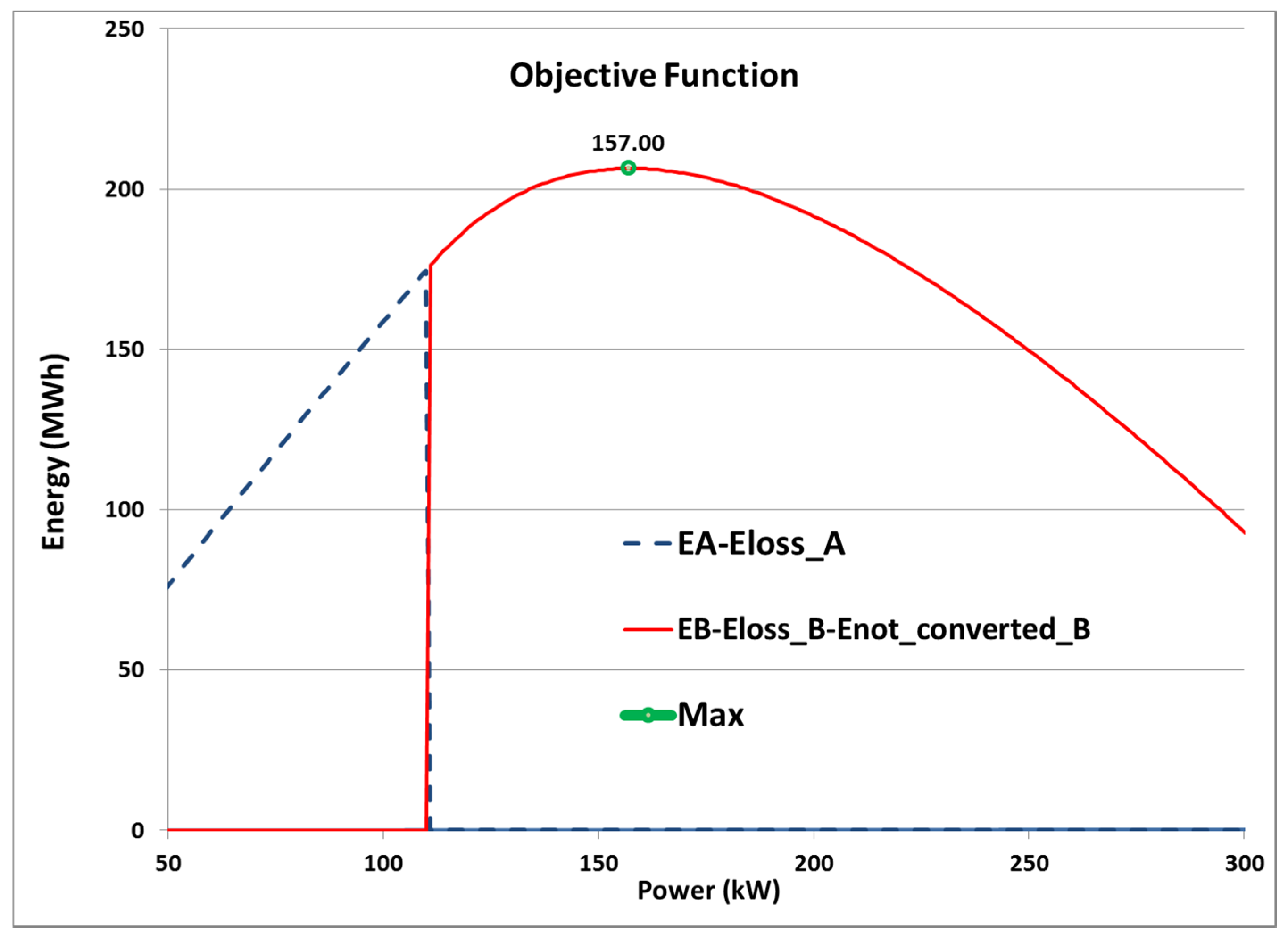
For instance, by using simulation results of Palermo, Italy, for a 100-kW inverter, the procedure has been evaluated, and Figure 6 shows the optimum point. Only through this energetic objective function, the maximum is reached when the P_PVpeak is slightly higher than the inverter size.

Figure 6. Objective function curve calculated for the city of Palermo, Italy.

Figure 6. Objective function curve calculated for the city of Palermo, Italy.

7. The Optimum PV Plant for a Specific Inverter: Simulation Result

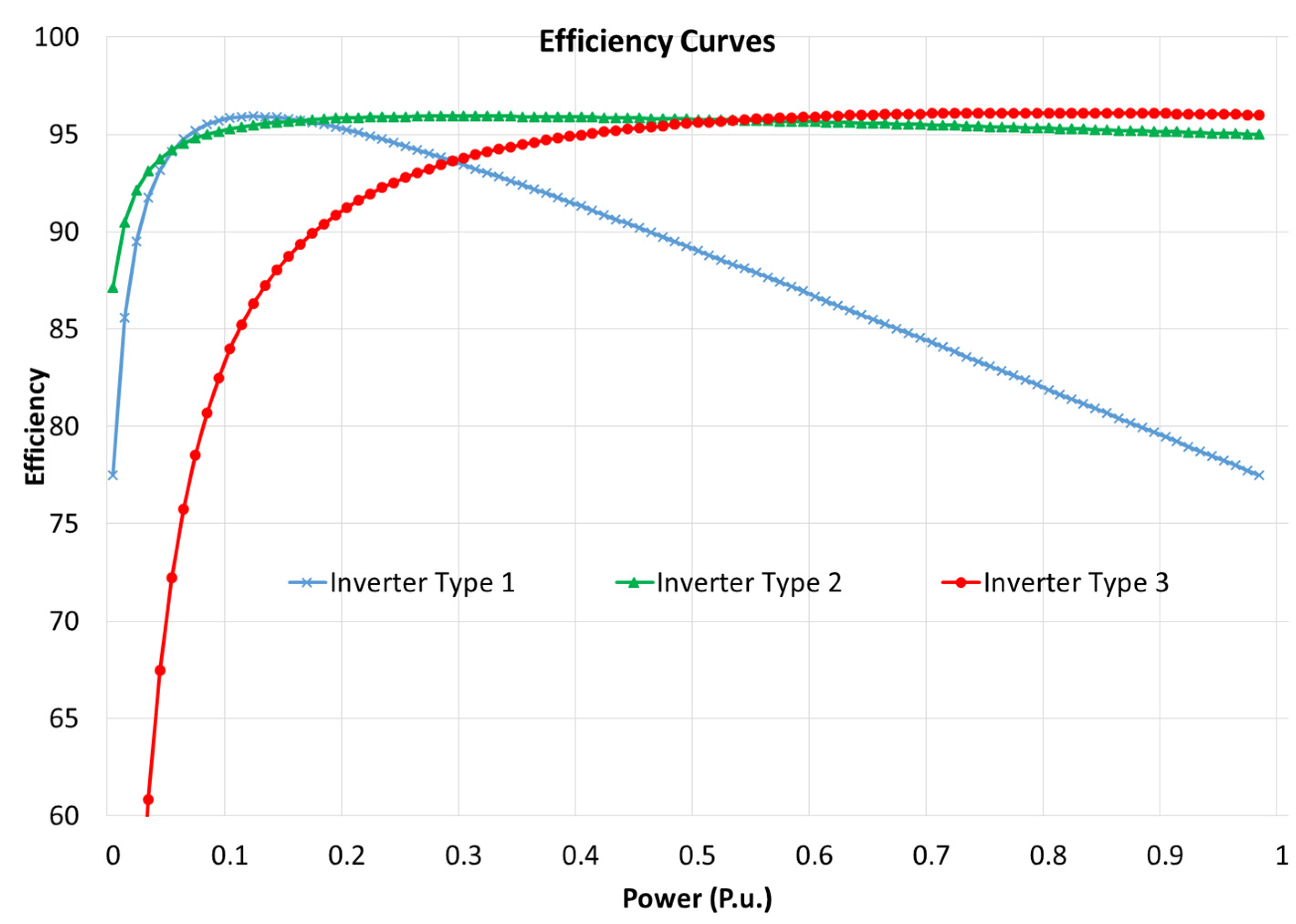
There exists a variety of types of solar inverters utilized in PV systems. These inverters can be categorized into three major types, which are introduced here;

-

Inverter Type 1: the inverter Type 1 has peak efficiency at a very low load percentage (14.1%) and, subsequently, a very waning curve;

-

Inverter Type 2: the inverter Type 2 reaches the maximum efficiency at a 31.6% load and keeps approximately constant performance up to the rated power;

-

Inverter Type 3: the inverter Type 3 has a peak performance at an 81.6% load, and once, it reaches the peak value, it performs almost as a constant curve.

Figure 7 shows the performance curves of the chosen inverters, as a function of the per unit DC-side power.

All other features of the three inverters are similar, and to ensure an effective comparison of the results, it is assumed that rated power, efficiency and the overload coefficient are fixed and equal for all three types:

-

P_nom (DC side) = 10 kW;

-

η_max = 96%;

-

k_s = 1 (overload coefficient).

According to the mathematical approximation for a solar inverter in Section 4, A, B and C coefficients are computed for the above-mentioned inverter. Results are presented in Table 3.

Figure 7. Example of three typical per unit efficiency curves for grid-connected solar inverters.

Figure 7. Example of three typical per unit efficiency curves for grid-connected solar inverters.

Table 3. Example of A, B, C coefficients of 3 solar inverter topologies.

Inverter type	A	B	C
Type 1	103.0	−25.0	−0.5
Type 2	97.2	−2.0	−0.2
Type 3	101.0	−3.0	−2.0

Table 3. Example of A, B, C coefficients of 3 solar inverter topologies.

Inverter type	A	B	C
Type 1	103.0	−25.0	−0.5
Type 2	97.2	−2.0	−0.2
Type 3	101.0	−3.0	−2.0

It should be noted that the coefficients A, B and C must be used in decimal form (not a percentage) for a correct application of the Equation (6). Table 4 presents simulation results of different latitudes for these inverters. It shows that inverter Type 1 has the lowest average ratio, because it works with high efficiency at low solar irradiance, which is more possible to occur for a solar inverter. Another important conclusion of Table 4 is that, for a specific inverter type, by increasing the latitude, the P_PVpeak/P_{nINV_DC} ratio is also increased.

Table 4. Power ratio between P_PVpeak/P_{nINV_DC} for different solar inverters and for different latitudes.

Type Ppvpeak/pninv_dc	Stockholm	Copenhagen	Paris	Palermo	Tripoli	Cairo	Average
Latitude	59.1°	55.4°	49.1°	38.0°	32.8°	30.1°	-
1	1.63	1.71	1.76	1.44	1.46	1.34	1.556
2	1.94	2.04	2.10	1.69	1.72	1.54	1.838
3	1.98	2.08	2.14	1.71	1.74	1.56	1.868

Table 4. Power ratio between P_PVpeak/P_{nINV_DC} for different solar inverters and for different latitudes.

Type Ppvpeak/pninv_dc	Stockholm	Copenhagen	Paris	Palermo	Tripoli	Cairo	Average
Latitude	59.1°	55.4°	49.1°	38.0°	32.8°	30.1°	-
1	1.63	1.71	1.76	1.44	1.46	1.34	1.556
2	1.94	2.04	2.10	1.69	1.72	1.54	1.838
3	1.98	2.08	2.14	1.71	1.74	1.56	1.868

Considering that most inverters on the market nowadays have Type 2 characteristics, by changing the latitude, the P_PVpeak/P_{nINV_DC} ratio is computed for the five different inverters (Type 2) represented in Section 4.

Since we considered the P_DC as the instantaneous DC power output from the PV modules, without any losses due to the transmission cables and without considering the inverter capability of being overloaded, these data represent the maximum power ratio available between P_PVpeak and P_{nINV_DC} for the latitudes shown in Table 5 at their optimum tilt angle.

Reminding that P_DCmax is related to P_PVpeak, Table 5 shows clearly how the power ratio between P_PVpeak and P_{nINV_DC} changes by latitude. Considering η_MAX from Table 2 and the calculated ratios in Table 5, it can be concluded that at each location, the inverter with higher η_MAX has a higher P_PVpeak/P_{nINV_DC} ratio or, in other words, that ratio multiplied by η_MAX is almost constant. With this consideration for each location, it is possible to define a constant. Then, by choosing the inverter type, the ratio can be computed by the average column in Table 5.

Table 5. Power ratio between P_PVpeak/P_{nINV_DC} for some solar inverters and for different latitudes.

Type	Stockholm	Copenhagen	Paris	Palermo	Tripoli	Cairo	Average
Latitude	59.1°	55.4°	49.1°	38.0°	32.8°	30.1°	-
I	1.91	1.99	2.06	1.66	1.69	1.52	1.805
II	1.95	2.04	2.11	1.69	1.72	1.54	1.842
III	1.95	2.04	2.11	1.69	1.72	1.55	1.843
IV	1.97	2.05	2.13	1.71	1.73	1.56	1.858
V	1.96	2.04	2.11	1.7	1.73	1.55	1.848
Average	1.948	2.032	2.104	1.690	1.718	1.544

Table 5. Power ratio between P_PVpeak/P_{nINV_DC} for some solar inverters and for different latitudes.

Type	Stockholm	Copenhagen	Paris	Palermo	Tripoli	Cairo	Average
Latitude	59.1°	55.4°	49.1°	38.0°	32.8°	30.1°	-
I	1.91	1.99	2.06	1.66	1.69	1.52	1.805
II	1.95	2.04	2.11	1.69	1.72	1.54	1.842
III	1.95	2.04	2.11	1.69	1.72	1.55	1.843
IV	1.97	2.05	2.13	1.71	1.73	1.56	1.858
V	1.96	2.04	2.11	1.7	1.73	1.55	1.848
Average	1.948	2.032	2.104	1.690	1.718	1.544

In this paper, the cost effect was not considered to find the optimum solution. By introducing the cost effect in the objective function, it seems that the ratio between P_PVpeak and P_{nINV_DC} could be lower than the ones obtained in this study. This consideration will be addressed in future works.

8. Conclusions

The comparison between monthly average and hourly average P_DC curve depicts that calculations based on the monthly average can inject considerable error into the design procedure. Therefore, this paper used the hourly average curve, which, in terms of accuracy and also the number of stored data, can be considered the best choice. Then, the optimum PV size, from the energy point of view, for a given inverter can be accurately calculated using the algebraic expressions developed in this paper, avoiding in this way multiple simulation efforts. The method developed in this study can be a valuable tool for design engineers comparing different inverters, calculating the optimum PV size of a given inverter type, estimating the annual AC energy yield and the effective annual inverter efficiency without performing multiple simulations. The validity of the proposed analytical model has been tested with the results obtained by simulations and measured data.

This study also showed the importance of defining a suitable function to consider all of the elements in order to find the optimum rated PV plant based on the power of the inverter and simultaneously to meet the power consumption requirements; for this reason, further works will regard the development of analytical expressions to estimate the optimum PV size for an inverter, by considering also costs and power requirements.