Modeling and Performance Analysis of State Transitions for Energy-Efficient Femto Base Stations ^†

Abstract

Lowering the energy required by base stations (BSs) is one of the hot issues nowadays in order to achieve green cellular networks. The energy consumption of femto BSs can be reduced, by turning off the radio interface when there is no mobile station (MS) under the coverage area of the femto BSs or MSs served by the femto BSs do not transmit or receive data packets for a long time, especially late at night. In the energy-efficient femto BSs, if MSs have any data packet to transmit and the radio interface of femto BSs is in the off state, MSs wake up the radio interface of femto BSs by using an additional low-power radio interface. In this paper, active (data), idle, active (signaling), sleep entering, sleep and waking up states are defined for the state model for the energy-efficient femto BSs, and the state transitions are modeled analytically. The steady-state probability of each state is derived thoroughly using a semi-Markov approach. Then, the performance of the energy-efficient femto BSs is analyzed in detail, from the aspects of energy consumption, cumulative average delay, cost and low-power radio signaling load. From the results, the tradeoff relationship between energy consumption and cumulative average delay is analyzed in detail, and it was concluded that an appropriate inactivity timer value should be selected to balance the tradeoff.

1. Introduction

Recently, the number of cellular subscribers and the traffic demand have been increased significantly due to the popularity of wireless Internet services, such as world wide web (WWW), instant messaging services, peer-to-peer (P2P) services, streaming services, etc. Due to the explosive growth of the data traffic for wireless Internet services using smart devices, such as smart phones and smart pads, the energy consumption of mobile stations (MSs) and base stations (BSs) is rapidly increasing, too [1–4]. Furthermore, the needs of the Internet of Things (IoT), which is based on wireless sensor networks, have increased significantly [5], and works on reducing the energy consumption of sensor nodes in wireless sensor networks have been carried out extensively, too [6,7]. Since the energy consumption of MSs and BSs produces large amounts of CO₂ emissions, works on reducing the energy consumption of MSs and BSs are being carried out actively in order to achieve green cellular networks [8–13].

Works on reducing the energy consumption of MSs have tried to extend the battery lifetime of MSs and, thus, reduce CO₂ emissions [8–10]. In these works, MSs stay in power saving mode or sleep mode, by turning off the radio interface when there is no data transmission with BSs. Then, MSs wake up periodically to check whether there is any incoming data packet to them and stay awake if there is any incoming data packet. Otherwise, MSs return to power saving mode or sleep mode to save energy.

Works on lowering the energy required by BSs have been carried out actively, too, in order to achieve green cellular networks [11–13]. In these works, the main idea of achieving green cellular networks is to sleep or turn off unused BSs to save energy, while supporting the coverage area of the sleep or turned off BSs by neighbor BSs. To achieve this goal, several schemes have been proposed, such as cell switching off [11], cell zooming [12] and cell wilting and blossoming [13]. In the cell switching off scheme [11], BSs are switched off when they are not necessary, since the traffic load is very low late at night, and the service area covered by the switched-off BSs is taken care of by the active neighbor BSs in order to guarantee service availability. In the cell zooming scheme [12], BSs adapt the cell size based on the varying traffic load. When the traffic load of a BS is congested, the cell size of the BS is reduced to escape from the traffic congestion. On the other hand, if the traffic load of a BS is very low, the cell size of the BS zooms out and the neighboring cells can zoom in. In the cell wilting and blossoming scheme [13], BSs go to the sleep state gradually by preventing any interruption of active data sessions (cell wilting), and MSs served by the wilting BS should be handed over to neighboring BSs. If the traffic load of any BS is higher than a threshold value, it alerts sleeping neighbor BSs, and then, the neighbor BSs wake up to cover the traffic load (cell blossoming). In these schemes, however, it is not easy to guarantee full service coverage all of the time, and thus, coverage hole problems may happen, which should be avoided for providing service availability to MSs.

In heterogeneous networks with macrocells and femtocells, the traffic load of macrocells is offloaded to femtocells, and the coverage hole problem can be avoided efficiently, since the full service coverage can be provided by overlay macrocells. In heterogeneous networks, macrocells and femtocells can use separate frequencies or share the same frequencies [14–17]. In these works on femtocells, the authors propose autonomous and coordinated resource allocation algorithms for interference mitigation based on cell transmit power minimization [14], the resource allocation scheme to maximize the capacity of delay-sensitive and delay-tolerant users subject to QoS and interference constraints [15], the cooperative Nash bargaining resource allocation scheme under the constraint of a cross-tier interference temperature limit to protect the primary macrocell and imperfect channel state information [16], spectrum efficient cognitive femtocell optimization with fairness and imperfect spectrum sensing [17] and a distributed and coordinated radio resource allocation algorithm which minimizes total downlink transmit power [18]. In a cognitive radio network, delay, hop count, power consumption, spectrum availability, route stability, interference, etc., are used for routing metrics [19]. Recently, the idea of using the unlicensed spectrum that is currently used by Wi-Fi for small cells has been proposed, too [20].

Femto BSs can turn off their radio interfaces without compromising the reachability of MSs and save energy when there is no MS under the coverage of the femto BSs or MSs do not transmit or receive data packet for a long time, especially late at night, as proposed in [21]. In [21], the authors use an additional low-power radio interface to wake up the radio interface of femto BSs in power saving mode [22] when MSs have any data to transmit via the femto BSs. By doing this, femto BSs can stay in a low-power state and serve MSs when the MSs request data transmission by waking up the radio interface of the femto BSs with the help of an additional low-power radio interface.

Although the performance of the energy-efficient femto BSs was analyzed using a testbed in [21], a detailed analysis of the effect of various parameters on the performance based on the state transition model was not dealt with analytically, to the best of our knowledge. In this paper, we propose a state model for energy-efficient femto BSs in [21] consisting of active (data), idle, active (signaling), sleep entering, sleep and waking up states and analyze the performance of the femto BSs, from the aspects of energy consumption, cumulative average delay, cost and low-power radio signaling load. We believe that the detailed mathematical analysis conducted in this paper based on the proposed state model is an essential first step to design a better power saving scheme for femto BSs. We note that although the state model of energy-efficient femto BSs was introduced and analyzed simply in our preliminary work [23], the work in this paper contains the following significant extensions:

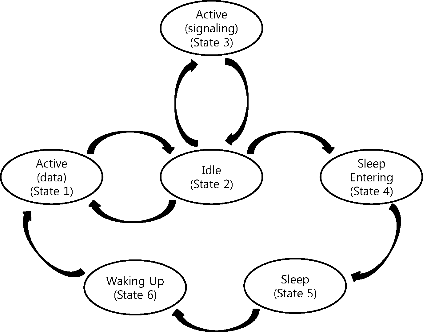
• A new state of active (signaling) is defined to accommodate the processing of location registrations of MSs.
• Two new states of sleep entering and waking up are defined to capture the energy consumptions of femto BSs when they are entering into the sleep state and waking up from the sleep state, which have higher energy consumptions than other states [24].
• A detailed analysis of the proposed state model is developed thoroughly, and a closed form of the steady-state probability of each state is derived completely.
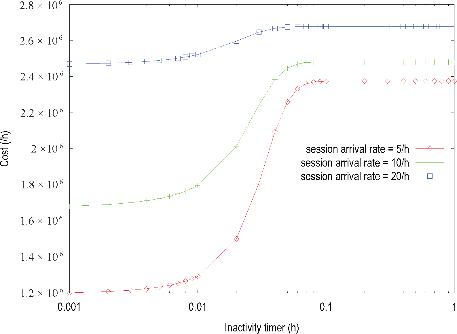
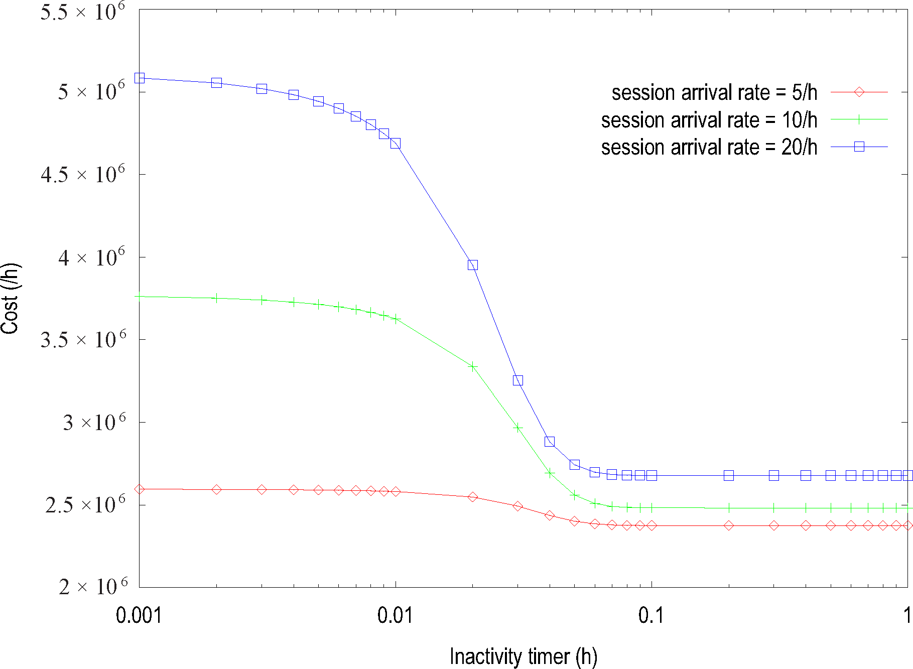
• The performance of the proposed state model is newly analyzed, from the aspect of cost, which is defined as a weighted sum of energy consumption and cumulative average delay.
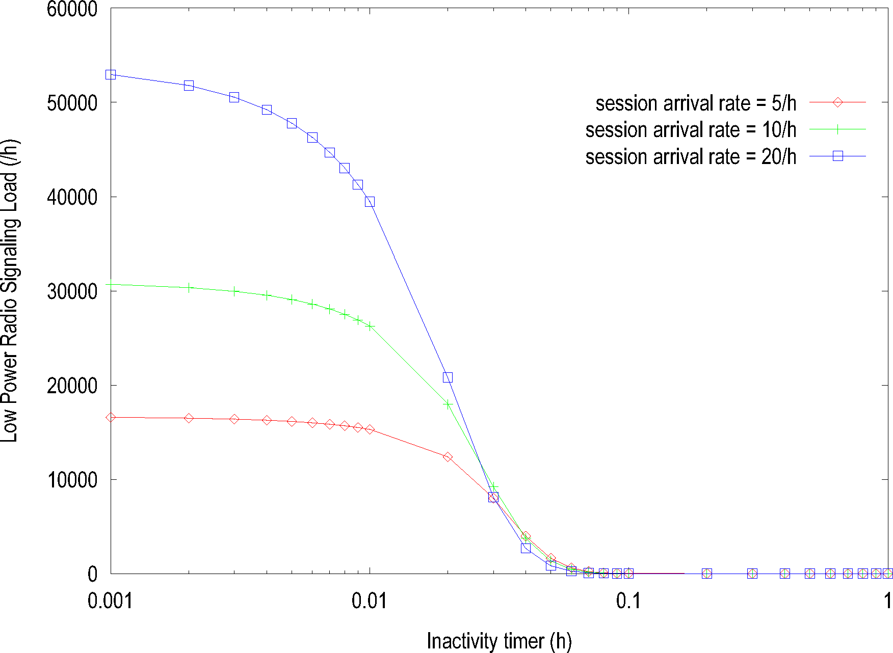
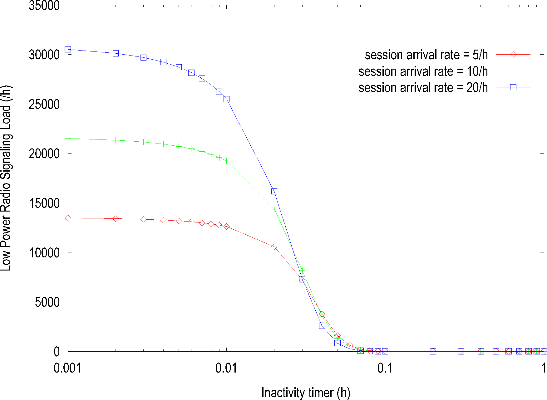
• The low-power radio signaling load of the proposed state model is newly analyzed, which is an overhead introduced in energy-efficient femto BSs.

Finally, the main contributions of this paper are summarized as follows:

• We proposed active (data), idle, active (signaling), sleep entering, sleep and waking up states for energy-efficient femto BS and formulated transition events between states.
• We derived a closed form of the steady-state probability of each state in the proposed state model analytically using a semi-Markov process approach.
• We presented an analytical framework for the performance analysis of the proposed state model, from the aspect of energy consumption, cumulative average delay, cost and low-power radio signaling load.
• We analyzed the effect of the the energy consumption of femto BSs when they are entering into the sleep state and waking up from the sleep state.
• The proposed analytical framework was validated by simulations.

The remainder of this paper is organized as follows: In Section 2, states for femto BSs are defined, and state transitions between them are modeled. Furthermore, the steady-state probability of each state is derived using a semi-Markov approach. Then, the performance of the energy-efficient femto BSs is analyzed in detail. In Section 3, numerical examples are provided, from the aspects of energy consumption, cumulative average delay, cost and low-power radio signaling load. Finally, conclusions and further works are drawn in Section 4.

2. Modeling and Analysis of State Transitions for Energy-Efficient Femto BS

2.1. Modeling of State Transitions

Figure 1 shows a proposed state transition model of femto BS considered in this paper, where the state of femto BS is divided into active (data), idle, active (signaling), sleep entering, sleep and waking up states. In the active (data) state, the radio interface of femto BSs is awake, and thus, BSs are sending or receiving data packets with MSs. In the active (signaling) state, the radio interface of femto BSs is awake similar to active (data) state, but this state is different from the active (data) state, since it only deals with location registration signaling, and thus, it has a very short service time compared to that of the active (data) state.

After completing service either in the active (data) state and active (signaling) state, the state returns to the idle state, and an inactivity timer is started. If there are no data or signaling transmission until the inactivity timer expires, the state moves to the sleep entering state, and the BSs start to turn off their radio interface and prepare to enter the sleep state. Otherwise, the inactivity timer is reset, and the state returns back to either the active (data) or active (signaling) state, depending on the type of activity, i.e., data or signaling transmission. That is, if data arrive, the state moves to the active (data) state. On the other hand, if signaling arrives, the state moves to the active (signaling) state.

If all of the necessary processing related to sleeping is completed in the sleep entering state, the state moves to the sleep state. In the sleep state, the energy of BSs can be saved significantly. If there is any data packet from MSs when the femto BS is in the sleep state, MSs send a reverse paging signal to wake up the femto BS by using an additional low-power radio interface [21]. As mentioned in [21], the low-power radio interface uses different radio channels with very low power, and thus, it does not consume the battery energy of MSs significantly. Then, the state moves to the waking up state and finally moves to the active (data) state, after completing all of the processing related to waking up. We note that we do not consider the transition from the sleep state to the active (signaling) state using a low-power radio interface, for simplicity, since using an additional low-power radio interface to wake up the femto BSs for location registration is not required necessarily, compared to data session processing.

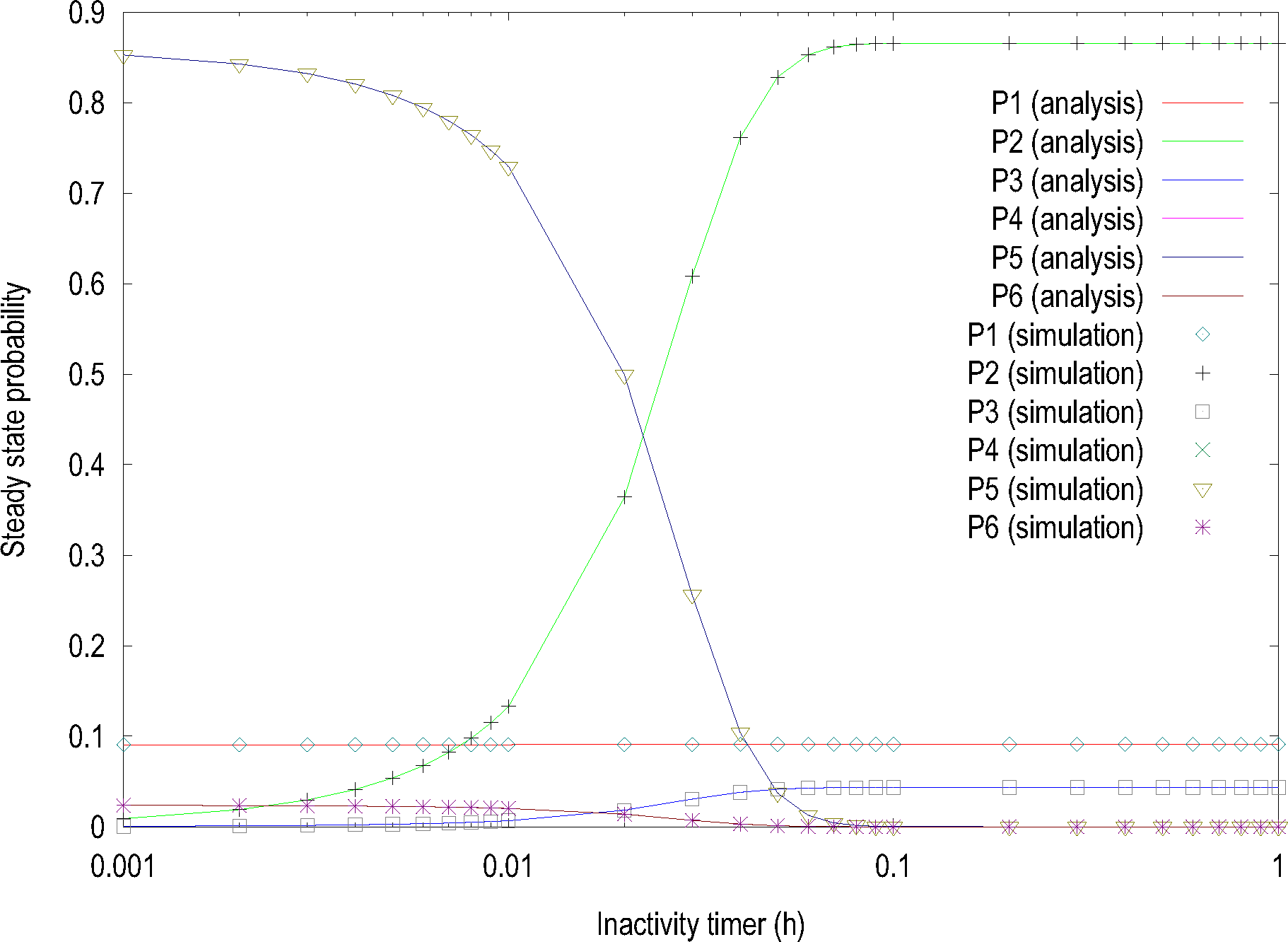
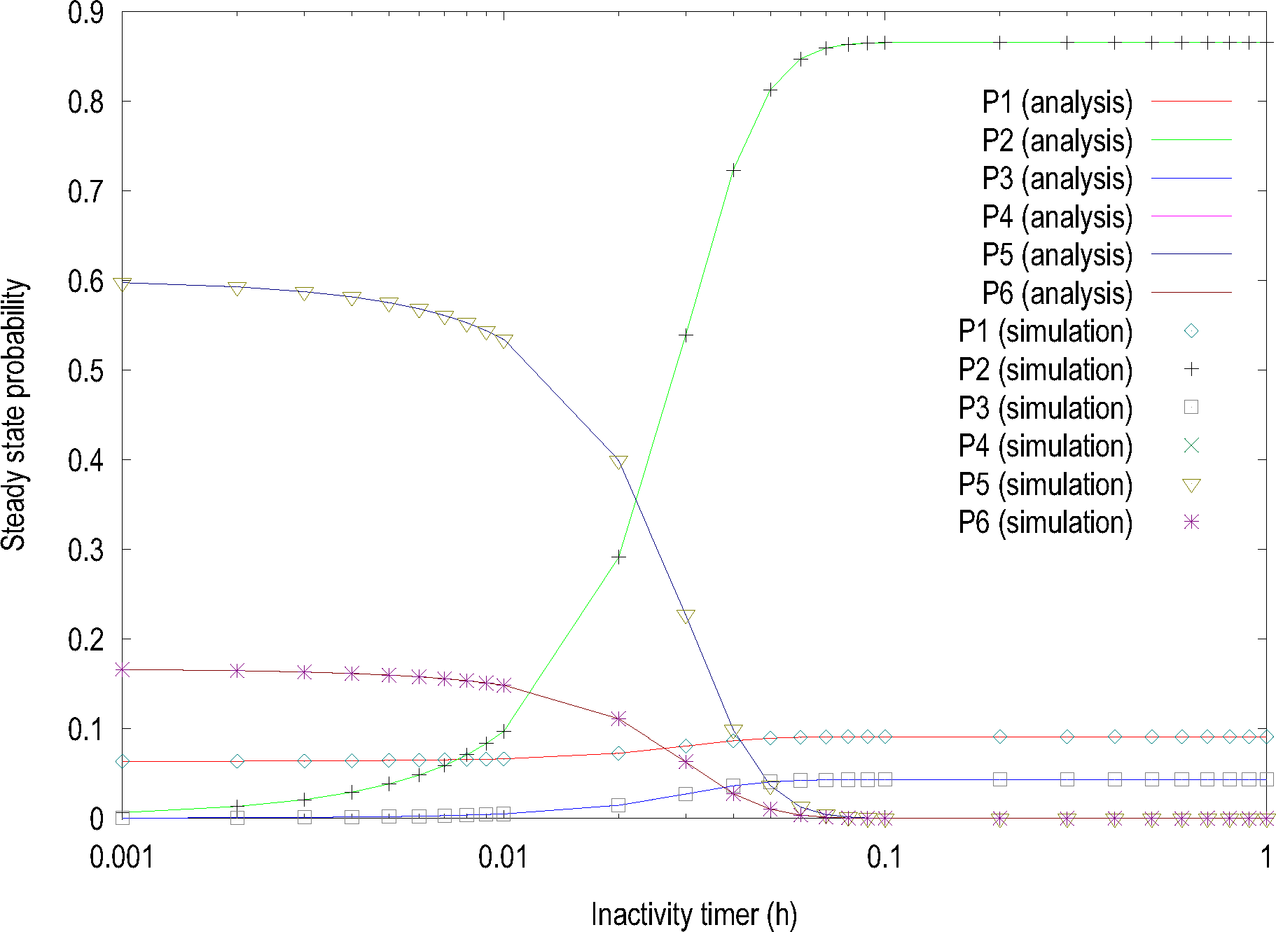
2.2. Performance Analysis

For the performance analysis, we have made the following assumptions regarding the density functions of random variables in each state:

• Session arrivals at an MS occur according to a Poisson process, and session arrivals at a femto BS from all of the MSs in the coverage of the femto BS occur according to a Poisson process with parameters λ_s;
• The time duration that a femto BS remains in the active (data) state follows a busy period of M/M/∞ queuing model;
• Location registration arrival at an MS occurs according to a Poisson process, and location registration arrivals at a femto BS from all of the MSs in the coverage of the femto BS occur according to a Poisson process with parameters λ_r;
• The time duration that a femto BS remains in the active (signaling) state follows an exponential distribution of μ_r, since it is assumed that the service time of a location registration signaling is very short compared to the inter-arrival time of two consecutive location registrations, and thus, more than one location registrations do not occur during the service time of the active (signaling) state;
• The value of inactivity timer is assumed as constant and is denoted by T_I.
• The time durations that a femto BS remains in the sleep entering and waking up states are assumed to be a fixed, and they are denoted by T_E and T_W, respectively [24].

We denote the active (data), idle, active (signaling), sleep entering, sleep and waking up states as States 1, 2, 3, 4, 5 and 6, respectively, for notational convenience. Since the residence times of all states of a femto BS do not follow an exponential distribution, the femto BS state transitions behavior is analyzed using a semi-Markov process approach [25].

The steady-state probability of each femto BS state can be obtained as:

$$P_k=\frac{{\pi }_k{\overline{t}}_k}{{\displaystyle {\sum }_{i=1}^6{\pi }_i{\overline{t}}_i}},k=1,2,3,4,5,\text{and}6$$

(1)

where π_k denotes the stationary probability of state k and ${\overline{t}}_k$ is the mean residence time of the femto BS in state k. The stationary probability is obtained by solving the following balancing equations [25]:

$${\pi }_j={\displaystyle \sum _{k=1}^6{\pi }_k{P}_{kj}},j=1,2,3,4,5,\text{and}6$$

(2)

$$1={\displaystyle \sum _{k=1}^6{\pi }_k}$$

(3)

where P_kj represents the state transition probability from state k to state j. The state transition probability matrix P = [p_kj] of the state transition model is given by Figure 1:

$$P=\left(\begin{array}{cccccc}0& P_{12}& 0& 0& 0& 0\\ P_{21}& 0& P_{23}& P_{24}& 0& 0\\ 0& P_{32}& 0& 0& 0& 0\\ 0& 0& 0& 0& P_{45}& 0\\ 0& 0& 0& 0& 0& P_{56}\\ P_{61}& 0& 0& 0& 0& 0\end{array}\right)$$

Then, stationary probabilities can be solved as:

$${\pi }_1=\frac{P_{21}+P_{24}+P_{45}+P_{56}+P_{61}}{Den}$$

(4)

$${\pi }_2=\frac{1}{Den}$$

(5)

$${\pi }_3=\frac{P_{23}}{Den}$$

(6)

$${\pi }_4=\frac{P_{24}}{Den}$$

(7)

$${\pi }_5=\frac{P_{24}{P}_{45}}{Den}$$

(8)

$${\pi }_6=\frac{P_{24}{P}_{45}{P}_{56}}{Den}$$

(9)

where Den is obtained by:

$$Den=1+P_{21}+P_{23}+P_{24}(1+P_{45}(1+P_{56}(1+P_{61})))$$

(10)

State transition probability P_kj can be derived based on the distribution of time from states k to j, T_kj. In the active (data), active (signaling), sleep entering, sleep and waking up states, since exits from these states occur due to only one event, P₁₂ = P₃₂ = P₄₅ = P₅₆ = P₆₁ = 1.

In the idle state, exit from idle is caused by any of the following three events:

• Data session arrival (T₂₁);
• Location registration signaling arrival (T₂₃);
• Inactivity timer expiration (T₂₄).

Then, the state transition probability P₂₁ is derived as:

$$\begin{array}{l}{P}_{21}={\displaystyle {\int }_0^{\infty }{f}_{T_{21}}(t)Pr(T_{23}>t)Pr}(T_{24}>t)dt\\ ={\displaystyle {\int }_0^{\infty }{\lambda }_s{e}^{-{\lambda }_{s}t}{e}^{-{\lambda }_{r}t}}{\displaystyle {\int }_t^{\infty }\delta (u-T_I)dudt}\\ ={\displaystyle {\int }_0^{\infty }{\lambda }_s{e}^{-({\lambda }_s+{\lambda }_r)t}U[T_I-t]}dt\\ ={\lambda }_s{\displaystyle {\int }_0^{T_I}{e}^{-({\lambda }_s+{\lambda }_r)t}}dt\\ =\frac{{\lambda }_s}{{\lambda }_s+{\lambda }_r}(1-e^{-({\lambda }_s+{\lambda }_r)T_I})\end{array}$$

(11)

Similarly, the state transition probability P₂₃ is derived as:

$$\begin{array}{l}{P}_{23}={\displaystyle {\int }_0^{\infty }{f}_{T_{23}}(t)Pr(T_{21}>t)Pr}(T_{24}>t)dt\\ ={\displaystyle {\int }_0^{\infty }{\lambda }_r{e}^{-{\lambda }_{r}t}{e}^{-{\lambda }_{s}t}}{\displaystyle {\int }_t^{\infty }\delta (u-T_I)dudt}\\ ={\displaystyle {\int }_0^{\infty }{\lambda }_r{e}^{-({\lambda }_s+{\lambda }_r)t}U[T_I-t]}dt\\ ={\lambda }_r{\displaystyle {\int }_0^{T_I}{e}^{-({\lambda }_s+{\lambda }_r)t}}dt\\ =\frac{{\lambda }_r}{{\lambda }_s+{\lambda }_r}(1-e^{-({\lambda }_s+{\lambda }_r)T_I})\end{array}$$

(12)

Finally, P₂₄ is obtained as:

$$P_{24}=1-P_{21}-P_{23}=e^{-({\lambda }_s+{\lambda }_r)T_I}$$

(13)

Now, we can derive the stationary probability of state k(i = 1, 2, 3, 4, 5 and 6) as follows:

$${\pi }_1=\frac{{\lambda }_s+{\lambda }_r{e}^{-({\lambda }_s+{\lambda }_r)T_I}}{({\lambda }_s+{\lambda }_r)(2+3e^{-({\lambda }_s+{\lambda }_r)T_I})}$$

(14)

$${\pi }_2=\frac{1}{2+3e^{-({\lambda }_s+{\lambda }_r)T_I}}$$

(15)

$${\pi }_3=\frac{{\lambda }_R(1-e^{-({\lambda }_s+{\lambda }_r)T_I})}{({\lambda }_s+{\lambda }_r)(2+3e^{-({\lambda }_s+{\lambda }_r)T_I})}$$

(16)

$${\pi }_4=\frac{e^{-({\lambda }_s+{\lambda }_r)T_I}}{2+3e^{-({\lambda }_s+{\lambda }_r)T_I}}$$

(17)

$${\pi }_5=\frac{e^{-({\lambda }_s+{\lambda }_r)T_I}}{2+3e^{-({\lambda }_s+{\lambda }_r)T_I}}$$

(18)

$${\pi }_6=\frac{e^{-({\lambda }_s+{\lambda }_r)T_I}}{2+3e^{-({\lambda }_s+{\lambda }_r)T_I}}$$

(19)

The mean residence time in the active (data) state is as follows, which is a busy period of the M/M/∞ model:

$${\overline{t}}_1=\frac{e^{{\lambda }_s/{\mu }_s}-1}{{\lambda }_s}$$

(20)

The mean residence time in the idle state is derived as:

$$\begin{array}{l}{\overline{t}}_2=\mathrm{E}[t_2]=\mathrm{E}[\min \{T_{21},T_{23},T_{24}\}]\\ ={\displaystyle {\int }_0^{\infty }\mathrm{Pr}(\min \{T_{21},T_{23},T_{24}\}>t)}dt\\ ={\displaystyle {\int }_0^{\infty }\mathrm{Pr}(T_{21}>t)\mathrm{Pr}(T_{23}>t)\mathrm{Pr}(T_{24}>t)}dt\\ ={\displaystyle {\int }_0^{\infty }{e}^{-{\lambda }_{s}t}{e}^{-{\lambda }_{r}t}}U(T_I-t)dt={\displaystyle {\int }_0^{T_I}{e}^{-({\lambda }_s+{\lambda }_r)t}}dt\\ =\frac{1-e^{-({\lambda }_s+{\lambda }_r)T_I}}{{\lambda }_s+{\lambda }_r}\end{array}$$

(21)

The mean residence time in the active (signaling) state is derived as:

$${\overline{t}}_3=\frac{1}{{\mu }_r}$$

(22)

The mean residence time in the sleep entering state is derived as:

$${\overline{t}}_4=T_E$$

(23)

The mean residence time in the idle sleep state is derived as:

$${\overline{t}}_5=\frac{1}{{\lambda }_s}$$

(24)

The mean residence time in the waking up state is derived as:

$${\overline{t}}_6=T_W$$

(25)

Based on the values of π_k and ${\overline{t}}_k$ obtained from Equations (4)–(9) and Equations (20)–(25), respectively, we finally derive the steady-state probability of each femto BS state using Equation (1). The steady-state probability of each state is derived as follows:

$$P_1=\frac{{\lambda }_s{\mu }_r^2({\lambda }_s+{\lambda }_r)(e^{{\lambda }_s/{\mu }_s}-1)({\lambda }_s+{\lambda }_r{e}^{-({\lambda }_s+{\lambda }_r)T_I})(2+3e^{-({\lambda }_s+{\lambda }_r)T_I})}{{\lambda }_s({\lambda }_r+{\mu }_r{e}^{{\lambda }_s/{\mu }_s})+({\mu }_r{\lambda }_r{e}^{{\lambda }_s/{\mu }_s}+{\lambda }_s({\mu }_r({\lambda }_s+{\lambda }_r)(T_E+T_W)-{\lambda }_r))e^{-({\lambda }_s+{\lambda }_r)T_I}}$$

(26)

$$P_2=\frac{{({\lambda }_s\mu )}^2({\lambda }_s+{\lambda }_r)(2+3e^{-({\lambda }_s+{\lambda }_r)T_I})(1-e^{-({\lambda }_s+{\lambda }_r)T_I})}{{\lambda }_s({\lambda }_r+{\mu }_r{e}^{{\lambda }_s/{\mu }_s})+({\mu }_r{\lambda }_r{e}^{{\lambda }_s/{\mu }_s}+{\lambda }_s({\mu }_r({\lambda }_s+{\lambda }_r)(T_E+T_W)-{\lambda }_r))e^{-({\lambda }_s+{\lambda }_r)T_I}}$$

(27)

$$P_3=\frac{{\lambda }_s^2{\lambda }_r{\mu }_r({\lambda }_s+{\lambda }_r)(2+3e^{-({\lambda }_s+{\lambda }_r)T_I})(1-e^{-({\lambda }_s+{\lambda }_r)T_I})}{{\lambda }_s({\lambda }_r+{\mu }_r{e}^{{\lambda }_s/{\mu }_s})+({\mu }_r{\lambda }_r{e}^{{\lambda }_s/{\mu }_s}+{\lambda }_s({\mu }_r({\lambda }_s+{\lambda }_r)(T_E+T_W)-{\lambda }_r))e^{-({\lambda }_s+{\lambda }_r)T_I}}$$

(28)

$$P_4=\frac{{({\lambda }_s{\mu }_r)}^2{({\lambda }_s+{\lambda }_r)}^2{T}_E(2+3e^{-({\lambda }_s+{\lambda }_r)T_I})e^{-({\lambda }_s+{\lambda }_r)T_I}}{{\lambda }_s({\lambda }_r+{\mu }_r{e}^{{\lambda }_s/{\mu }_s})+({\mu }_r{\lambda }_r{e}^{{\lambda }_s/{\mu }_s}+{\lambda }_s({\mu }_r({\lambda }_s+{\lambda }_r)(T_E+T_W)-{\lambda }_r))e^{-({\lambda }_s+{\lambda }_r)T_I}}$$

(29)

$$P_5=\frac{{\lambda }_s{\mu }_r^2{({\lambda }_s+{\lambda }_r)}^2{T}_E(2+3e^{-({\lambda }_s+{\lambda }_r)T_I})e^{-({\lambda }_s+{\lambda }_r)T_I}}{{\lambda }_s({\lambda }_r+{\mu }_r{e}^{{\lambda }_s/{\mu }_s})+({\mu }_r{\lambda }_r{e}^{{\lambda }_s/{\mu }_s}+{\lambda }_s({\mu }_r({\lambda }_s+{\lambda }_r)(T_E+T_W)-{\lambda }_r))e^{-({\lambda }_s+{\lambda }_r)T_I}}$$

(30)

$$P_6=\frac{{({\lambda }_s{\mu }_r)}^2{({\lambda }_s+{\lambda }_r)}^2{T}_W(2+3e^{-({\lambda }_s+{\lambda }_r)T_I})e^{-({\lambda }_s+{\lambda }_r)T_I}}{{\lambda }_s({\lambda }_r+{\mu }_r{e}^{{\lambda }_s/{\mu }_s})+({\mu }_r{\lambda }_r{e}^{{\lambda }_s/{\mu }_s}+{\lambda }_s({\mu }_r({\lambda }_s+{\lambda }_r)(T_E+T_W)-{\lambda }_r))e^{-({\lambda }_s+{\lambda }_r)T_I}}$$

(31)

Now, we can obtain the energy consumption of a femto BS per unit hour in the proposed state model by using the steady-state probability as:

$$E=3600\times {\displaystyle \sum _{k=1}^6{\psi }_k}{P}_k$$

(32)

where ψ_k is the power consumption of a femto BS in state k.

Although transition into the sleep state can save energy, additional delay is introduced for session initiation, since MSs must wake up femto BSs and obtain new IP address using DHCP [21]. Therefore, there is tradeoff between energy consumption and delay, and thus, the effect of delay introduced by turning off the radio interface of BSs should be analyzed. In this paper, cumulative average delay per unit hour in the proposed state model is obtained as:

$$D=3600\times \left(D_{on}\frac{P_2{P}_{21}}{{\overline{t}}_2}+D_{off}{P}_5/{\overline{t}}_5\right)$$

(33)

where D_on and D_off are the delay needed to initiate a new data session in the idle and sleep states, respectively.

Since there is tradeoff between energy consumption and cumulative average delay, we define a cost as a weighted sum of energy consumption and cumulative average delay in order to analyze the tradeoff as follows:

$$C=3600\times (w_{energy}E+w_{delay}D)$$

(34)

where w_energy and w_delay are weight factors for energy consumption and cumulative average delay, respectively. The approach of using a weighted sum is used widely in the literature in order to compare the effect of factors that have different units.

Finally, the low-power radio signaling load is obtained as:

$$S=3600\times (P_3/{\overline{t}}_3)$$

(35)

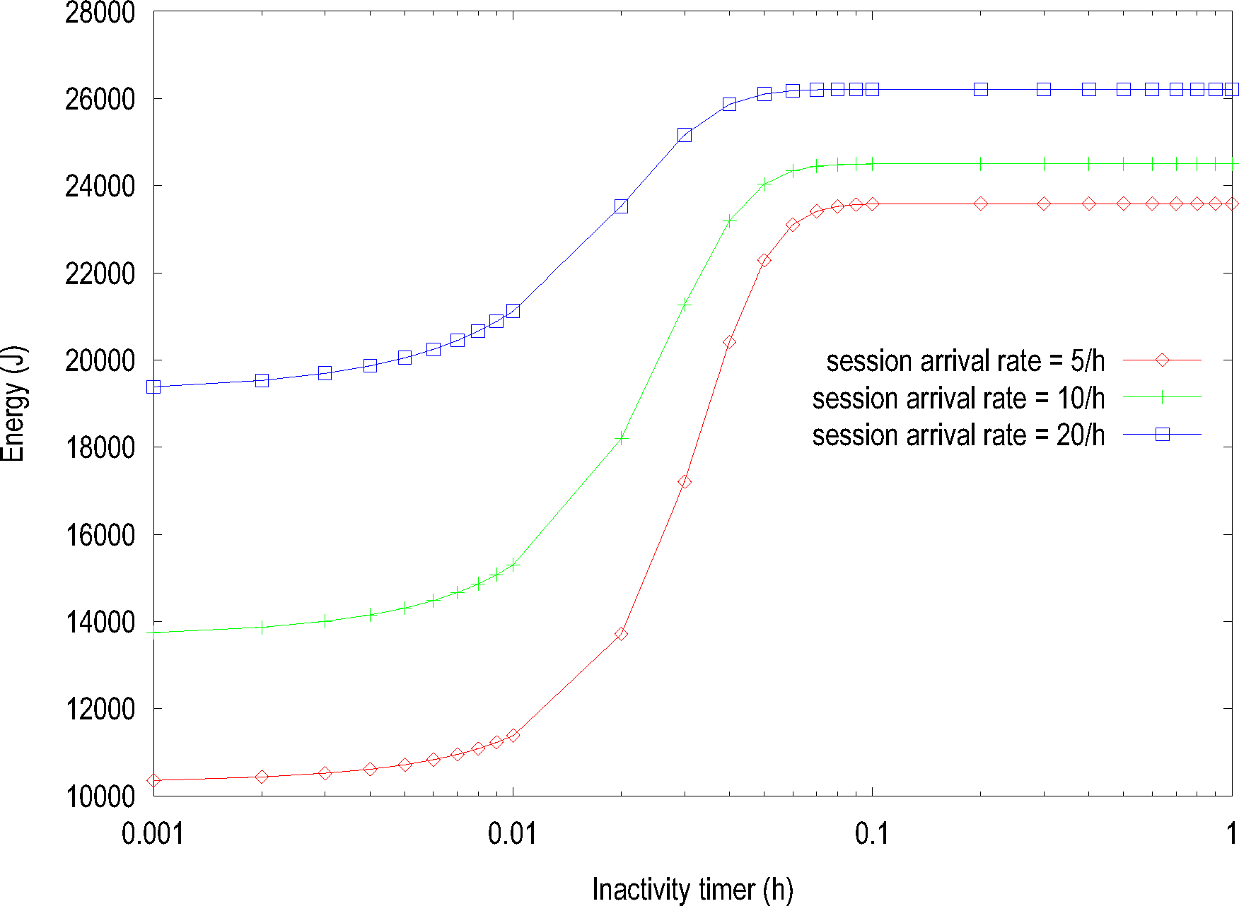
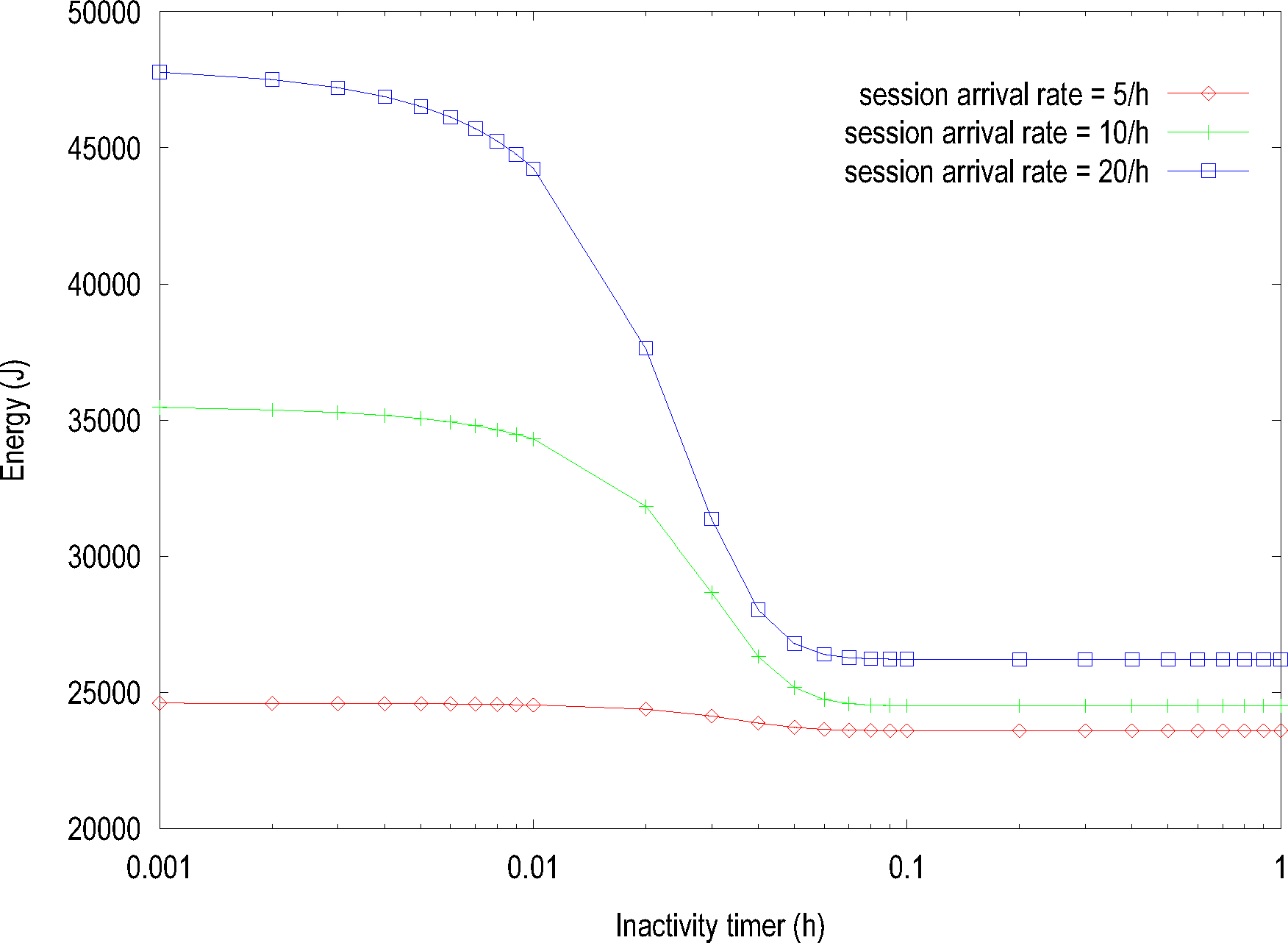
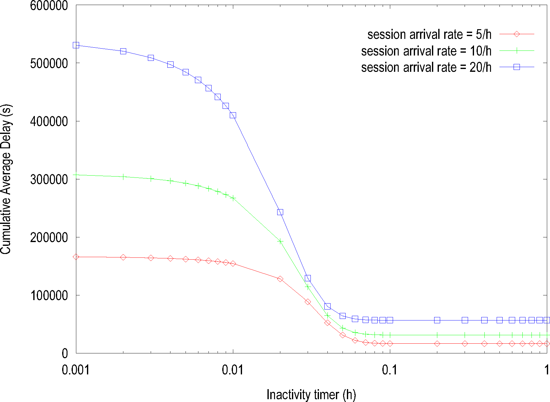
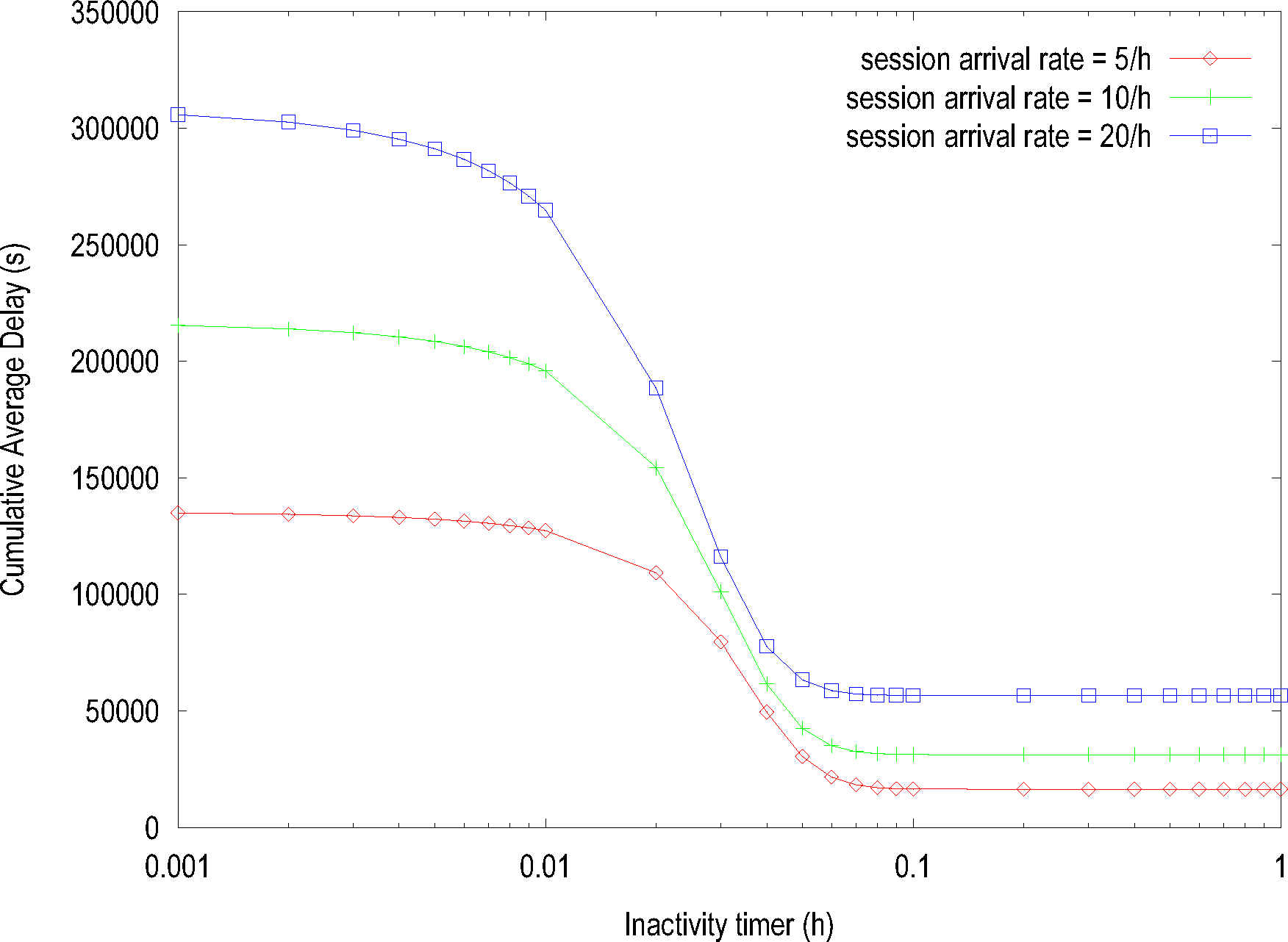
3. Numerical Examples

In the numerical examples, we show the energy consumption, cumulative average delay, cost and low-power radio signaling load for varying the values of inactivity timer. Furthermore, the effect of the energy consumption of entering into the sleep state and waking up from the sleep state is analyzed by considering two different time duration sets for T_E and T_W.

Figure 2 shows the steady-state probability of the femto BS state by varying the values of inactivity timer T_I with λ_s = 10 (/h), μ_s = 100 (/h), λ_r = 100 (/h), μ_r = 2000 (/h), ψ₁ = 12 W, ψ₂ = 6 W, ψ₃ = 12 W, ψ₄ = 24 W, ψ₅ = 1.2 W, ψ₆ = 24 W, T_E = 10/3600 (h) and T_W = 10/3600 (h). The figure shows both analysis and simulation results, and we can see that the analysis result is validated by simulation results. The probability of the idle state increases as the values of the inactivity timer increase due to less transitions into the sleep state. On the other hand, the probability of the sleep state decreases as the values of the inactivity timer increase. Furthermore, the probability of active is almost constant and does not highly depend on the values of the inactivity timer, since transition into the active state occurs from both idle and sleep states, which have the opposite probability distributions. The probability of the active (signaling) state increases as the values of the inactivity timer increase, similar to that of the idle state, since the transition into the active (signaling) state occurs from the idle state. The probabilities of sleep entering and waking up are the same and decrease as the values of the inactivity timer increases, similar to that of the sleep state, but they have much smaller probability values. From the results, we can see that the value of the inactivity timer has a significant effect on the steady-state probability of the femto BS state.

Figure 3 shows the steady-state probability of the femto BS state by varying the values of the inactivity timer T_I with the same parameter values, except for T_E = 100/3600 (h) and T_W = 100/3600 (h). The figure shows both analysis and simulation results, and we can see that the analysis result is validated by simulation results. The distributions of probabilities of states in this figure are very similar to those in Figure 2. However, the probabilities of the sleep entering and waking up states are higher than those in Figure 2, since MSs stay in these states for a longer time duration. On the other hand, the probability of the sleep state decreases due to increased mean residence time, i.e., steady-state probability, in the sleep entering and waking up states.

Figure 4 and Figure 5 show the energy consumption by varying the values of the inactivity timer T_I and the rate of data session arrival λ_r, with the same parameter settings as those of Figure 2 and Figure 3, respectively. The energy consumption of Figure 4 increases as the values of the inactivity timer increase, since the probability of the idle state increases, which has a higher power consumption than the sleep state, and the effects of energy consumptions of the sleep entering and waking up states are not significant due to the small mean residence times, i.e., steady-state probabilities, of these states. On the other hand, the energy consumption of Figure 5 decreases as the values of the inactivity timer increase, since the effects of energy consumptions of the sleep entering and waking up states are significant due to the increased mean residence times, i.e., steady-state probabilities, of these states, although the probability of the idle state increases, similar to Figure 4. These results show that different inactivity timer values should be selected appropriately to reduce energy consumptions depending on the effect of the energy consumptions of the sleep entering and waking up states. For a fixed value of the inactivity timer, the energy consumption increases as the rate of session arrival increases, in both Figure 4 and Figure 5, since higher data session arrivals cause more transitions into the active (data) state. From the results, we can see that an appropriate value for the inactivity timer should be selected to reduce energy consumption, depending on the energy consumption in the sleep entering and waking up states.

Figure 6 and Figure 7 show the cumulative average delay by varying the values of the inactivity timer T_I and the rate of data session arrival λ_r, with the same parameter settings as those of Figure 2 and Figure 3, respectively, except for D_off = 10(s) and D_on = 1(s). The shapes of the cumulative average delay in Figure 6 and Figure 7 are very similar to each other, but the delay in Figure 6 has higher values, since the probability of the sleep state is higher in Figure 6. The cumulative average delay decreases as the values of the inactivity timer increase, since the probability of the idle state increases, which has a smaller delay than the sleep state. For a fixed value of the inactivity timer, the cumulative average delay increases as the rate of data session arrival increases. For small values of the inactivity timer, the effect of long delay in the sleep state is more dominant. Otherwise, the effect of short delay in the idle state is more dominant.

Figure 8 and Figure 9 show the cost by varying the values of the inactivity timer T_I and the rate of data session arrival λ_r, with the same parameter settings as those of Figure 2 and Figure 3, respectively, except for D_off = 10(s), D_on = 1(s), w_energy = 20 and w_delay = 1. The cost of Figure 8 increases as the values of the inactivity timer increase, since the effect of energy consumption is more dominant in the considered setting of weight factors, and the energy consumption of femto BSs decreases, as the values of the inactivity timer increase, as shown in Figure 4. On the other hand, the cost of Figure 9 decreases as the values of the inactivity timer increase, since the effect of energy consumption is more dominant in the considered setting of weight factors, and the energy consumption of femto BSs increases, as the values of the inactivity timer increase, as shown in Figure 5. For a fixed value of the inactivity timer, the cost increases as the rate of session arrival increases, in both Figure 8 and Figure 9, since higher data session arrivals cause more energy consumptions and cumulative average delays. From the results, we can see that an appropriate value for the inactivity timer should be selected to reduce the cost, depending on the energy consumption in the sleep entering and waking up states.

Figure 10 and Figure 11 show low-power radio signaling load by varying the values of the inactivity timer T_I and the rate of data session arrival λ_r, with the same parameter settings as those of Figure 2 and Figure 3, respectively. The signaling load decreases as the values of the inactivity timer increase, since the signaling load is proportional to the probability of the sleep state, which decreases as the values of the inactivity timer increase. The shapes of signaling load in Figures 10 and 11 are very similar to each other, but the signaling load in Figure 10 has higher values, since the probability of the sleep state is higher in Figure 10. For a fixed value of the inactivity timer, the signaling load increases as the rate of session arrivals increases, in both Figure 10 and Figure 11, since higher data session arrivals cause more waking up from the sleep states.

4. Conclusions and Further Works

In this paper, the state model for energy-efficient femto BSs is proposed, and the performance of the proposed state model is analyzed, from the aspects of energy consumption, cumulative average delay, cost and low-power radio signaling load. From the results, the tradeoff relationship between energy consumption and cumulative average delay was shown. Furthermore, the tradeoff between them was analyzed by using a cost, which is defined as a weighted sum of energy consumption and cumulative average delay. Numerical results showed that a smaller value of the inactivity timer is preferable for small values of T_E and T_W, and a larger value of the inactivity timer is preferable for large values of T_E and T_W. Therefore, an appropriate inactivity timer value should be selected appropriately to balance the tradeoff. In our further works, the power saving of MSs should be considered together with that of BSs, and thus, the integrated power saving of MSs and BSs will be analyzed.

References

1. Hasan, Z.; Boostanimehr, H.; Bhargava, V.K. Green cellular networks: A survey, some research issues and challenges. IEEE Commun. Surv. Tutor. 2011, 13, 524–540. [Google Scholar]
2. Suarez, L.; Nuaymi, L.; Bonnin, J.M. An overview and classification of research approaches in green wireless networks. EURASIP J. Wirel. Commun. Netw. 2012, 2012, 1–18. [Google Scholar]
3. Bianzino, A.P.; Chaudet, C.; Rossi, D.; Rougier, J.L. A survey of green networking research. IEEE Commun. Surv. Tutor. 2012, 14, 3–20. [Google Scholar]
4. Wang, X.; Vasilakos, A.V.; Chen, M.; Liu, Y.; Kwon, T.T. A survey of green mobile networks: Opportunities and challenges. Springer Mob. Netw. Appl. 2012, 4–20. [Google Scholar]
5. Sheng, Z.; Yang, S.; Yu, Y.; Vasilakos, A.V.; McCann, J.A.; Leung, K.K. A survey on the IETF protocol suite for the Internet of things: standards, challenges, and opportunities. IEEE Wirel. Commun. 2013, 20, 91–98. [Google Scholar]
6. Han, K.; Luo, J.; Liu, Y.; Vasilakos, A.V. Algorithm design for data communications in duty-cycled wireless sensor networks: A survey. IEEE Commun. Mag. 2013, 51, 107–113. [Google Scholar]
7. Yao, Y.; Cao, Q.; Vasilakos, A.V. EDAL: An energy-efficient, delay-aware, and lifetime-balancing data collection protocol for heterogeneous wireless sensor networks. IEEE/ACM Trans. Netw. 2014, PP. [Google Scholar] [CrossRef]
8. Kwon, S.W.; Cho, D.H. Dynamic power saving mechanism for mobile station in the IEEE 802.16e Systems, Proceedings of the 2009 IEEE 69th Vehicular Technology Conference (2009 VTC Spring), Barcelona, Spain, 26–29 April 2009.
9. Zhou, L.; Xu, H.; Tian, H.; Gao, Y.; Du, L.; Chen, L. Performance analysis of power saving mechanism with adjustable DRX cycles in 3GPP LTE, Proceedings of the IEEE 68th Vehicular Technology Conference (2008 VTC 2008-Fall), Calgary, BC, Canada, 21–24 September 2008.
10. He, Y.; Yuan, R. A novel scheduled power saving mechanism for 802.11 wireless LANs. IEEE Trans. Mob. Comput. 2009, 8, 1368–1383. [Google Scholar]
11. Marsan, M.A.; Chiaraviglio, L.; Ciullo, D.; Meo, M. Optimal energy savings in cellular access networks, Proceedings of the IEEE International Conference on Communications Workshops (ICC Workshops 2009), Dresden, Germany, 14–18 June 2009.
12. Niu, Z.; Wu, Y.; Gong, J.; Yang, Z. Cell zooming for cost-efficient green cellular networks. IEEE Commun. Mag. 2010, 48, 74–79. [Google Scholar]
13. Conte, A.; Feki, A.; Chiaraviglio, L.; Ciullo, D.; Meo, M.; Marsan, A. Cell wilting and blossoming for energy efficiency. IEEE Wirel. Commun. 2011, 18, 50–57. [Google Scholar]
14. Lopez-Perez, D.; Chu, X.; Vasilakos, A.V.; Claussen, H. Power minimization based resource allocation for interference mitigation in OFDMA femtocell networks. IEEE J. Sel. Areas Commun. 2014, 32, 333–344. [Google Scholar]
15. Zhang, H.; Jiang, C.; Beaulieu, N.C.; Chu, X.; Wen, X. Resource allocation in spectrum-sharing OFDMA femtocells with heterogeneous services. IEEE Trans. Commun. 2014, 62, 2366–2377. [Google Scholar]
16. Zhang, H.; Jiang, C.; Beaulieu, N.C.; Chu, X.; Wang, X.; Quek, T.Q.S. Resource allocation for cognitive small cell networks: A cooperative bargaining game theoretic approach. IEEE Trans. Wirel. Commun. 2015. [Google Scholar] [CrossRef]
17. Zhang, H.; Jiang, C.; Mao, X.; Chen, H.H. Interference-limited resource optimization in cognitive femtocells with fairness and imperfect spectrum sensing. IEEE Trans. Vehicular Technol. 2015. [Google Scholar] [CrossRef]
18. Lopez-Perez, D.; Chu, X.; Vasilakos, A.V.; Claussen, H. On distributed and coordinated resource allocation for interference mitigation in self-organizing LTE networks. IEEE Trans. Netw. 2013, 21, 1145–1158. [Google Scholar]
19. Youssef, M.; Ibrahim, M.; Abdelatif, M.; Chen, L.; Vasilakos, A.V. Routing metrics of cognitive radio networks: A survey. IEEE Commun. Surv. Tutor. 2014, 16, 92–109. [Google Scholar]
20. Zhang, H.; Chu, X.; Guo, W.; Wang, S. Coexistence of Wi-Fi and heterogeneous small cell networks sharing unlincensed spectrum. IEEE Commun. Mag. 2015, 53, 158–164. [Google Scholar]
21. Haratcherev, I.; Balageas, C.; Fiorito, M. Low consumption home femto base stations, Proceedings of the 2009 IEEE 20th International Symposium on Personal, Indoor and Mobile Radio Communications, Tokyo, Japan, 13–16 September 2009.
22. Gu, L.; Stankovic, J. Radio-triggered wake-up for wireless sensor networks. Real Time Syst. 2005, 29, 157–182. [Google Scholar]
23. Chung, Y.W. Performance analysis of energy-efficient home femto base stations, Proceedings of the International Conference on Electrical, Computer, Electronics and Communication Engineering, Paris, France, 24–26 June 2011.
24. Wang, D.; McNair, J.; George, A. A smart-NIC-based power-proxy solution for reduced power consumption during instant messaging, Proceedings of the IEEE Green Technologies Conference Grapevine, TX, USA, 15–16 April 2010.
25. Ross, S.M. Stochastic Processes; John Wiley & Sons: Hoboken, NJ, USA, 1996. [Google Scholar]
Figure 1. State transition model of the femto base station.
Energies 08 04629f1
Figure 2. Steady-state probability by varying the session arrival rate (small values of TE and TW).
Energies 08 04629f2
Figure 3. Steady-state probability by varying the session arrival rate (large values of TE and TW).
Energies 08 04629f3
Figure 4. Energy consumption by varying the session arrival rate (small values of TE and TW).
Energies 08 04629f4
Figure 5. Energy consumption by varying the session arrival rate (large values of TE and TW).
Energies 08 04629f5
Figure 6. Cumulative average delay by varying the session arrival rate (small values of TE and TW).
Energies 08 04629f6
Figure 7. Cumulative average delay by varying the session arrival rate (large values of TE and TW).
Energies 08 04629f7
Figure 8. Cost by varying session the arrival rate (small values of TE and TW).
Energies 08 04629f8
Figure 9. Cost by varying the session arrival rate (large values of TE and TW).
Energies 08 04629f9
Figure 10. Low-power radio signaling load by varying the session arrival rate (small values of TE and TW).
Energies 08 04629f10
Figure 11. Low-power radio signaling load by varying the session arrival rate (large values of TE and TW).
Energies 08 04629f11