Experimental Results of a DC Bus Voltage Level Control for a Load-Controlled Marine Current Energy Converter

Abstract

This paper investigates three load control methods for a marine current energy converter using a vertical axis current turbine (VACT) mounted on a permanent magnet synchronous generator (PMSG). The three cases are; a fixed AC load, a fixed pulse width modulated (PWM) DC load and DC bus voltage control of a DC load. Experimental results show that the DC bus voltage control reduces the variations of rotational speed by a factor of 3.5 at the cost of slightly increased losses in the generator and transmission lines. For all three cases, the tip speed ratio λ can be kept close to the expected λ_opt. The power coefficient is estimated to be 0.36 at λ_opt; however, for all three cases, the average extracted power was about ∼ 19%. A maximum power point tracking (MPPT) system, with or without water velocity measurement, could increase the average extracted power.

1. Introduction

Control systems for vertical axis turbines (VAT) with permanent magnet synchronous generators (PMSG) in renewable energy with an intermittent primary resource typically operate by rectifying the generator voltages and controlling the rotational speed of the turbine using the DC bus voltage. There are a few different ways of trying to achieve maximum power point tracking (MPPT) once the turbine has reached the nominal operation region. Different electronic components are required depending on the application.

There is not much published in the area of control methods for VAT with PMSG in marine currents, but it has been a popular field of research the last two decades for vertical axis wind turbines (VAWT) with PMSG. A common way of compensating for the wide range of voltage levels in wind power applications is to use a DC/DC converter or a tap transformer [1,2,3]. Control of a VAWT with PMSG using tip speed ratio control is suggested in [4,5]. A method for finding the optimal operation point without wind speed measurement nor turbine parameters is presented in [6]. Using the rotational speed of the turbine as the wind speed measurement is suggested in [7]. Combining MPPT and tip speed ratio control is presented in [8].

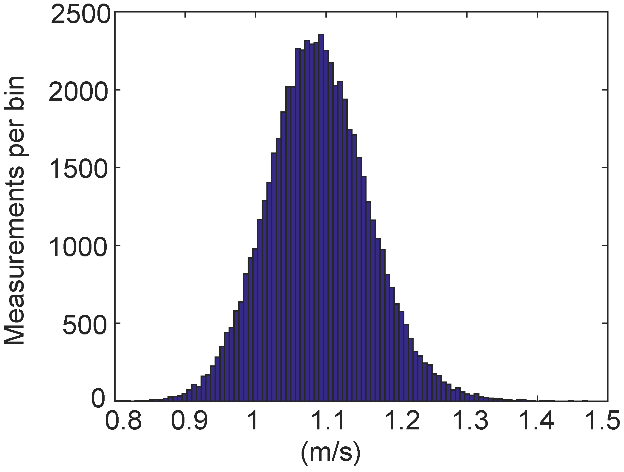
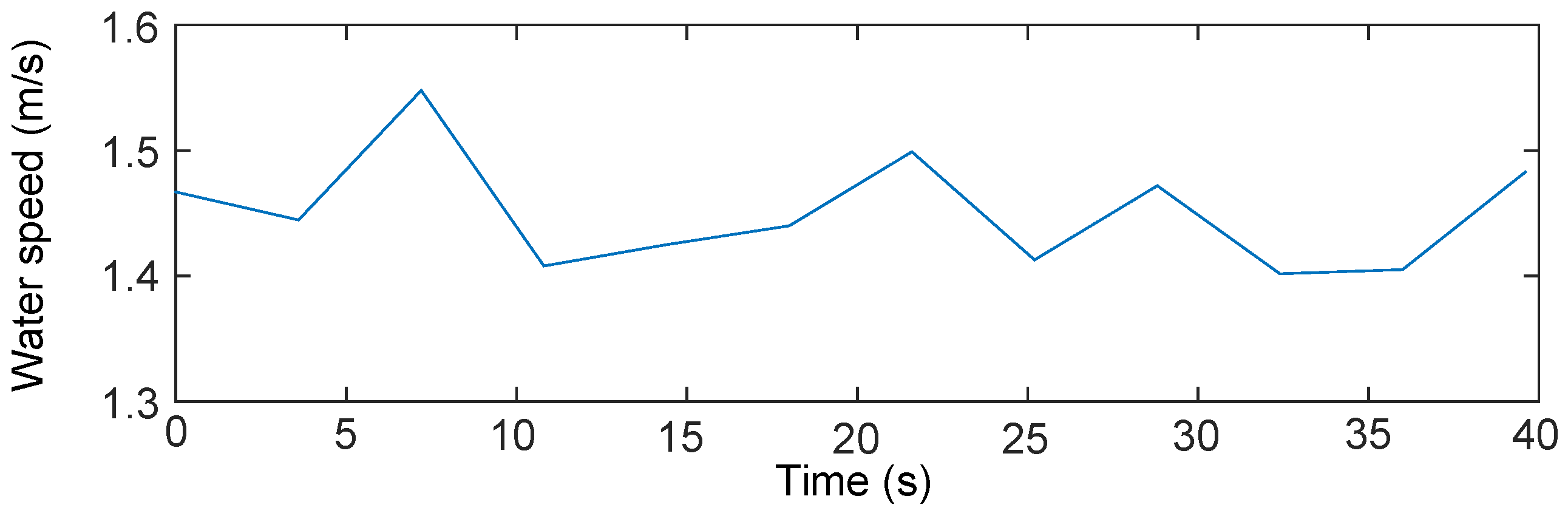
Marine current energy conversion is in many ways similar to wind energy conversion, but there are a number of significant differences. On p. 53 of [9], we see that during 45 s of wind speed measurements, the variation of wind speed is from 4 m/s to 7 m/s. Figure 1 shows typical speed measurements during 40 s for marine currents. There is clearly a large difference in characteristics between the two; in particular, the highest and lowest values obtained during the relatively short time span differ much more for wind than for currents. For a direct drive system in these conditions, the difference in power absorption (and output voltage) between the high and the low velocity would be bigger for wind power. This would suggest that the optimal design of a control system for a marine current power generator would be different from that of wind power, which, in turn, indicates the need for research on control systems for marine current applications.

Figure 1. Water velocity upstream of the Söderfors turbine on 16 April 2014.

Figure 1. Water velocity upstream of the Söderfors turbine on 16 April 2014.

This paper reports an investigation of voltage control of the DC bus of a VAT with PMSG in a marine application. Two control methods using load control are evaluated and compared to a fixed AC load case. Various benefits and drawbacks of the different strategies will be discussed against the background of the measured performance of each method. The purpose is to publish experimental results of the control system implemented in the experimental setup and to provide guidance for further development of control systems of VAT with PMSG in marine applications.

1.1. Load Control in Marine Current Power Applications

The power in a flowing fluid over a cross-section with area A is:

$$P_{kinetic}=\frac{1}{2}A\mathrm{\rho }{v}^3$$

(1)

where v is water speed and ρ is the density of water. The fraction of power delivered to the generator from the turbine is called the power coefficient, C_P , defined as:

$$C_P=\frac{P_{turbine}}{P_{kinetic}}$$

(2)

C_P is a function of the tip speed ratio λ, i.e., the ratio of blade speed to undisturbed water speed, defined as:

$$\lambda =\frac{\Omega r}{v}$$

(3)

where Ω is the rotational speed of the turbine and r the turbine radius. Maximum power extraction from the water, C_Pmax, occurs at some optimal tip speed ratio λ_opt. The mechanical power P_turbine delivered to the generator by the turbine shaft is converted to electricity. It is consumed by the load and dissipated as losses in the generator, bearings and the transmission lines; see more in Section 3.2. At steady-state, it can be written as:

P_turbine ∼ P_losses + P_load

(4)

Combining (1), (2) and (4), we see that:

$$\frac{1}{2}{C}_P\rho A{v}^3 \sim P_{losses}+P_{load}$$

(5)

and since C_P = C_P (λ), by varying the load, we can control the rotational speed of the turbine. This way, the system can be kept at λ_opt and the greatest amount of energy from the water can be extracted.

Defining the system efficiency, η_system, as average electric power delivered over the average power available in the water,

$${\eta }_{system}=\frac{<P_{turbine}>}{<P_{kinetic}>}$$

(6)

This implies that the overall performance of the electrical power generation system will be dependent on the ability of the control system to keep the rotational speed Ω of the turbine at (or as close as possible to) the speed corresponding to λ_opt.

2. The Söderfors Experimental Station

The Marine Current Power Group at Uppsala University operates an experimental power station in the river Dal (Dalälven) at Söderfors, Sweden, deployed in 2013 [10]. The experimental station comprises a turbine, a generator and a measurement cabin (housing control and measurement systems).

The turbine is placed in the outlet channel of a conventional hydropower plant at a distance of approximately 800 m and at a depth of 7 m. It has five vertical blades with a NACA0021 profile, 3.5 m in height and 0.18 m in chord length. The turbine radius is 3 m. The generator is a directly-driven permanent magnet synchronous generator. At nominal operation (rotational speed of 15 revolutions per minute (RPM) at a water speed of 1.3 m/s), the generator delivers a line-to-line RMS voltage of 138 V and a 31 A RMS current for a total power rating of 7.5 kW. The design optimal tip speed ratio is λ_opt = 3.5. The generator is connected to the measurement cabin on shore by a power cable some 200 m long.

The experimental station is more fully described in [11,12]. A more detailed description of the generator can be found in [13]. Further details of the control and measurement system can be found in [14].

2.1. ADCP Measurements

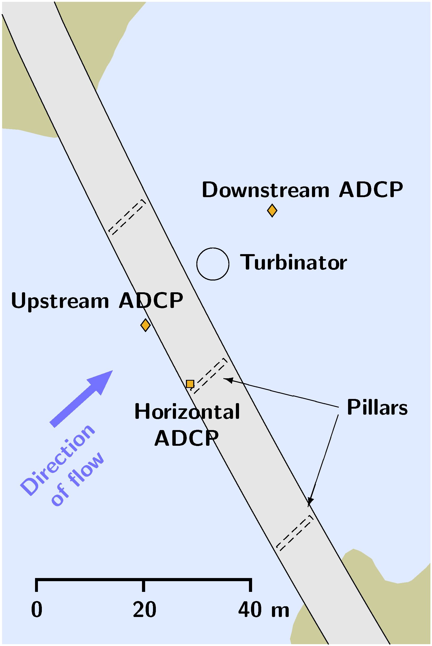
Three acoustic Doppler current profilers (ADCPs) are permanently installed at the test site (see Figure 2). Two of them are vertically oriented, placed on the riverbed about 15 m upstream and 15 m downstream of the turbine, and the third one is horizontally oriented and located upstream. The vertical devices are Workhorse Sentinel 1200 Hz with an accuracy of 0.3% of the water speed. Measurements are taken every few seconds (set by the user) and give a velocity profile from one meter above the bottom of the river to one meter below the surface at 0.25 m intervals. Mean velocity magnitude values from the upstream and downstream vertical ADCPs are used in this paper.

Figure 2. An overview of the test site. The river reach is part of the outlet channel from a hydropower plant. The turbinator is placed immediately downstream of a road bridge. Vertically-oriented ADCPs are placed on the riverbed upstream and downstream of the turbinator. A horizontally-oriented ADCP is mounted on a bridge pillar upstream.

Figure 2. An overview of the test site. The river reach is part of the outlet channel from a hydropower plant. The turbinator is placed immediately downstream of a road bridge. Vertically-oriented ADCPs are placed on the riverbed upstream and downstream of the turbinator. A horizontally-oriented ADCP is mounted on a bridge pillar upstream.

2.2. Electrical Layout

The only sensors inside the generator are Hall sensors for detecting rotational speed and a camera supported by LED lights. All other electrical measurements are made inside the measurement cabin.

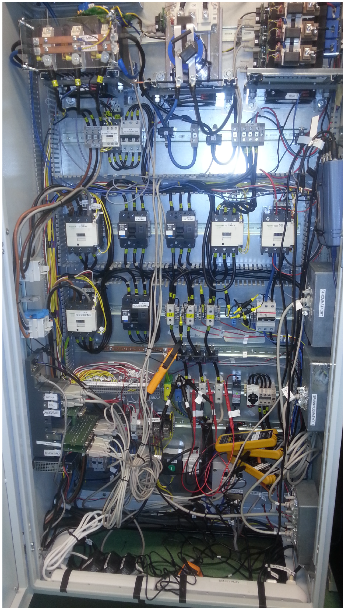
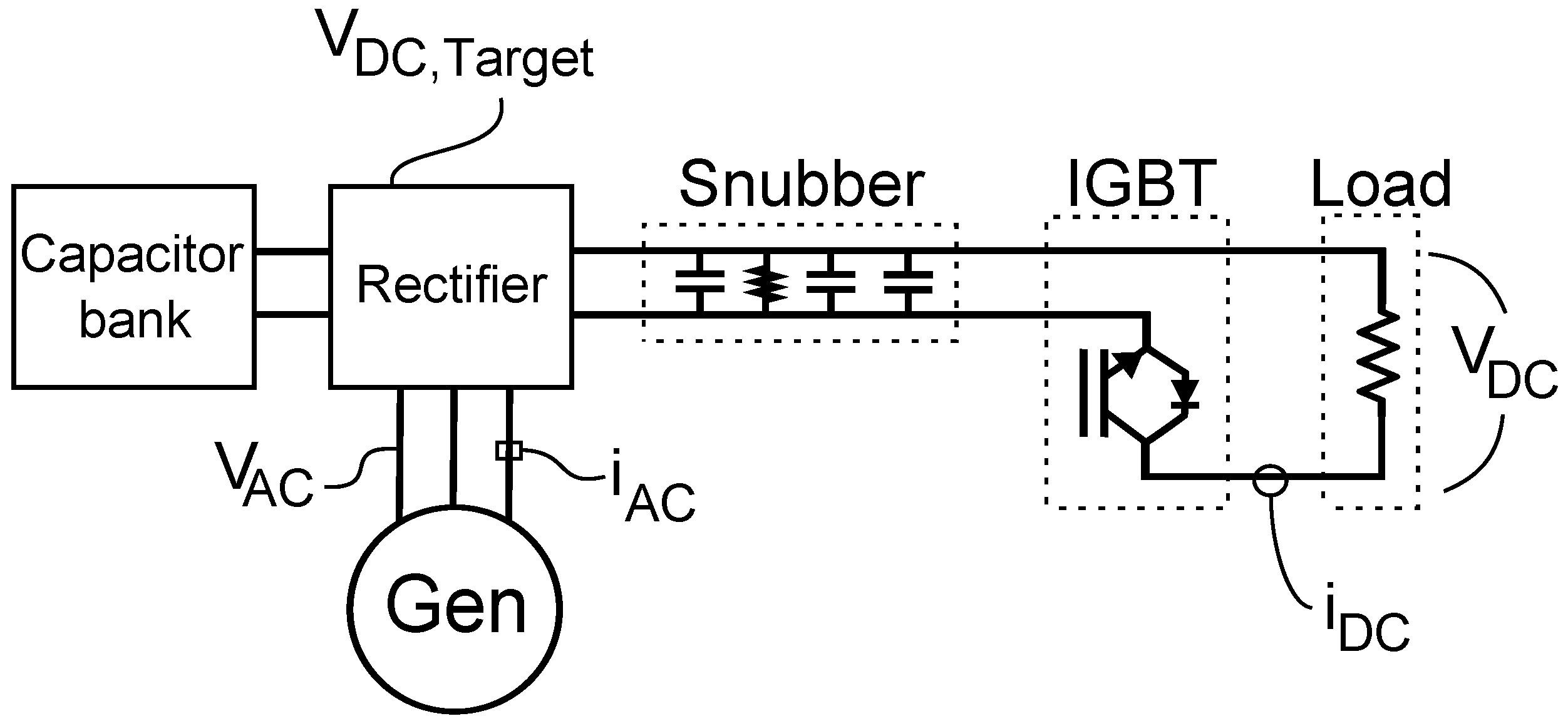
An enclosure containing all electrical components is located in the measurement cabin; see Figure 3. The entire system is controlled using a CompactRIO and LabView. The generator windings double as a startup circuit, and contactors in the enclosure are used for connecting the load control system once sufficient rotational speed has been reached during startup. Manual switches are used to (prior to startup) connect a fixed resistive load either in an AC three-phase Wye connection or a DC connection. The DC load comprises the resistive load, a rectifier with a capacitor bank and an insulated-gate bipolar transistor (IGBT) with a snubber circuit in parallel (see Figure 4). The rectifier is a passive diode rectifier using Semikron SKKD 100/16 diodes, and the capacitor bank consists of 12 capacitors of 2.2 µF connected in parallel to achieve a total of 26.4 mF. The IGBT is a Semikron SKM400GAL12V module, and the snubber circuit uses a Vishay 3300 µF UR 450 V capacitor, two Vishay 470 nF 386M MKP capacitors and a RIFA PYR 47 kΩ resistor.

The power electronics input voltages, line-to-neutral and line-to-line, are measured inside the measurement cabin. AC currents are sensed with HAL 100 and HAL 200 current sensors from LEM and read to an NI 9205 module in the CompactRIO. DC currents and voltages are measured in/over the load and read to a PicoScope with Fluke i310s AC/DC Current Clamps and Teledyne Lecroy AP031 Differential Probes.

Figure 3. The electrical enclosure.

Figure 3. The electrical enclosure.

Figure 4. The DC load control consisting of a rectifier, capacitor bank, IGBT with a snubber circuit and resistive load.

Figure 4. The DC load control consisting of a rectifier, capacitor bank, IGBT with a snubber circuit and resistive load.

2.3. Load Control System

The AC load comprises no electrical control during operation. Once the switch from the startup circuit to the load has been made, the generator is connected directly to the AC load.

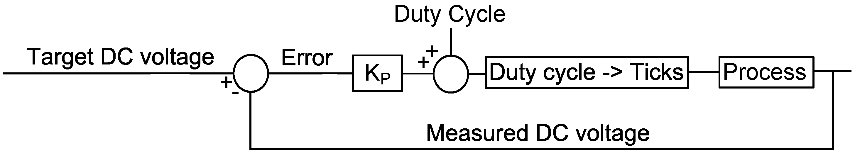
The DC load operation uses the FPGA module of the CompactRIO to control the switching frequency of the IGBT. Two control algorithms have been implemented for DC load control: constant duty cycle and target DC voltage. The constant duty cycle is an open loop controller where the user sets a desired duty cycle (see Figure 5). The target DC voltage aims to keep the DC bus voltage constant using a P-controller loop (see Figure 6). The FPGA operates at 40 MHz, and time is converted to ticks in the LabView software. One second is 40 million ticks, i.e., the duty cycle and PWM frequency will each correspond to a number of ticks. The control loop runs every 100 ticks.

Figure 5. Open loop controller of the DC load duty cycle.

Figure 5. Open loop controller of the DC load duty cycle.

Figure 6. P-controller loop of the DC bus voltage.

Figure 6. P-controller loop of the DC bus voltage.

3. Methodology

The three methods are referred to as follows: The AC load case is the AC case; the fixed PWM DC load is the fixed PWM; and the target DC voltage control is the constant DC. Each control strategy was used during 30 minutes of operation and was evaluated by the variation in rotational speed, losses and the extracted electric power. An average value of the ADCP measurements was used to calculate the average power absorbed by the turbine. The variation of the delivery of power to the DC bus was determined using Equations (3) and (5) and the rotational speed. For each load case, the average power consumed in the load, the transmission lines and the generator windings was calculated. Average power P from a series of N measurements of momentary current i_n was calculated as:

$$P=\frac{1}{N}\sum _{n=1}^{N}R·i_n^2$$

(7)

where R is the circuit resistance. The power in the AC transmission lines and in the generator is assumed to be equally divided over the three phases, so the total power can be calculated as power in one phase multiplied by three.

The design point λ_opt = 3.5 was used together with an average value of the water velocity to determine at which RPM to switch over to load control. Data were recorded starting a few minutes after the desired RPM had been reached, in order to build up a wake behind the turbine.

3.1. Load Control Parameters

For both of the DC control cases, a PWM frequency of 500 Hz was used. A duty cycle of 17% was used in the fixed PWM case, and in the constant DC case, the target DC voltage was set to 173.5 V and K_P = 1.

3.2. Losses

In this paper, mechanical losses in bearings and seals, as well as iron losses (eddy current, hysteresis and dynamic losses) in the generator are not analysed.

The mechanical losses are due to friction in the bearings and seals and are therefore linearly dependent on the rotational speed. Since the generator operates at roughly the same speed in the three cases studied, the losses can be considered equal in magnitude for the purposes of this study.

The electrical losses in the iron in the generator are described by the following equations: Power loss from eddy currents is described by P_eddy = $k_e{B}_{max}^2{f}^2{d}^{2}V [W]$, where k_e is an eddy current coefficient, B_max the maximum flux density, d the thickness of the laminations and V is the stator volume. Power loss from hysteresis is described by P_hysteresis = $k_h{B}_{max}^{2}fV$, where k_h is a constant that includes the material properties. Power loss from the excess dynamic loss component is described by P_excess = k_ex (B_maxf)^3/2 V , where k_ex is a material constant. These three quantities are not dependent on the power drawn in the generator, but only on the frequency, f. Since the rotational speed is roughly the same in the whole study, iron losses can be assumed to be approximately equal in all three cases.

Since the study is aimed at comparing differences among the three control cases, losses that are equal in all cases do not contribute to the results. In conclusion, the losses analysed in this study are assumed to be purely resistive and only in the transmission lines and generator windings. The resistance is measured using a Rhopoint M210 milliohm meter with an accuracy of 0.1% of measuring range.

3.3. Water Velocity Measurements Using ADCPs

The turbine is located between the two ADCP devices. The cross-section of the river at the upstream device and the downstream is not the same. That means that if the discharge is the same at both points, the velocity will not be the same. However, since the river reach is in fact the man-made outlet channel from a hydropower plant, the geometric variation is not very dramatic. If we assume that the turbine is located exactly midway between the upstream and downstream ADCPs and that the change in cross-section is linear, we can use the average value of the fraction of the upstream and downstream device,

C = v_upstream/v_downstream

(8)

to estimate the velocity at the turbine, v. This average value of C can be used to find a correction factor, c, so that the velocity of the water at the turbine can be written as:

v = v_upstream · c

(9)

Then, the average power at the turbine can be calculated as:

$$<P_{kinetic}>=\frac{1}{N}{\displaystyle \sum _{n=1}^N\frac{1}{2}}A\rho v_n^3$$

(10)

As it should not make a difference if the downstream or the upstream values are used, here it was decided to use the upstream values for all measurements, v(v_upstream, c); see Equation (9).

4. Results

4.1. ADCP Measurements for the Correction Factor

One week of measurements from the upstream and downstream devices was recorded during the week leading up to the AC and DC load experiments, with a frequency of 0.1 Hz. Figure 7 shows a histogram of C , and the average value was C_mean = 1.090. Equation (9) gives c = 0.9587 and the velocity of the water at the turbine can now be estimated as v = 0.9587 · v_upstream.

Figure 7. Histogram of the fraction of the upstream and the downstream measurements during one week.

Figure 7. Histogram of the fraction of the upstream and the downstream measurements during one week.

4.2. ADCP Measurements for the Load Cases

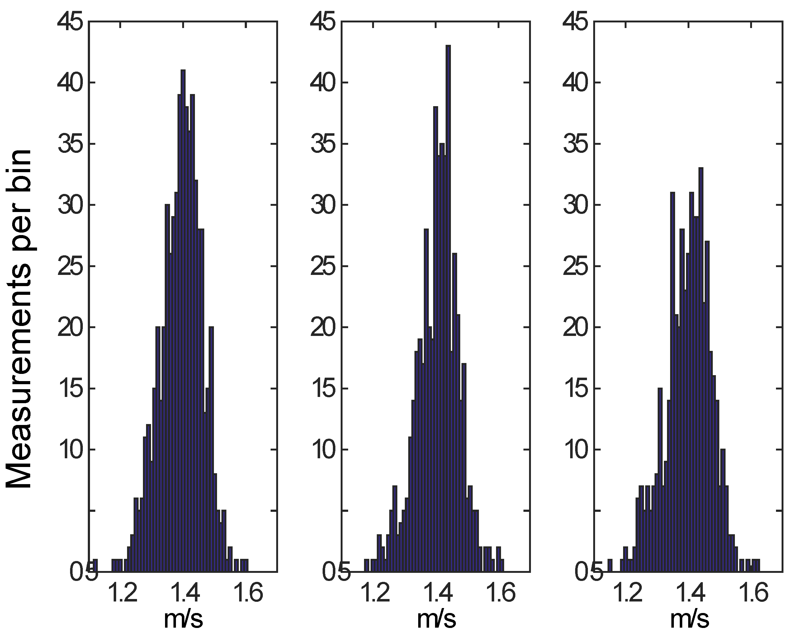
Table 1 shows the average values of v_upstream and v. The calculated average power at the turbine was calculated using Equation (10), the measured water speed with correction factor c, A = 21 m² and ρ=1000 kg/m³. Figure 8 shows a histogram of v_upstream, where the measurement was done at (1/3.6) Hz.

Table 1. Average velocity measured by the ADCP and calculated average power across the turbine at the respective speeds.

Load Case	AC	Fixed PWM	Constant DC
vupstream (m/s)	1.394	1.406	1.399
Variance (m/s)	0.005	0.005	0.005
Measurement points	601	501	502
v (m/s)	1.336	1.348	1.341
Mean Pkinetic (kW)	27.44	28.15	27.78

Table 1. Average velocity measured by the ADCP and calculated average power across the turbine at the respective speeds.

Load Case	AC	Fixed PWM	Constant DC
vupstream (m/s)	1.394	1.406	1.399
Variance (m/s)	0.005	0.005	0.005
Measurement points	601	501	502
v (m/s)	1.336	1.348	1.341
Mean Pkinetic (kW)	27.44	28.15	27.78

Figure 8. Histogram of water speed during load conditions. From left to right: AC load, fixed PWM and constant DC.

Figure 8. Histogram of water speed during load conditions. From left to right: AC load, fixed PWM and constant DC.

A statistical analysis will determine if the three load case measurements were made during similar conditions. For all three cases, a one-sample Kolmogorov–Smirnov test with a p-value of 0.05 rejects the hypothesis that the velocities come from a normal distribution. A Levene test can investigate the variance in non-normal distributions. The Levene test with a p-value of 0.05 cannot reject that the variances in the three cases are equal. The Wilcoxon signed rank test with a p-value of 0.05 rejects a zero median in difference in mean values between the AC load case and the fixed PWM case, but cannot reject the other two cases. This means that the variation in the water velocities was equal for the three cases, but the average water velocity was higher for the fixed PWM case than for the AC case. As seen in Table 1, there was a higher number of measurements made for the AC case. This does not affect the result of the statistical analysis, since the number of measurements made is included in the tests.

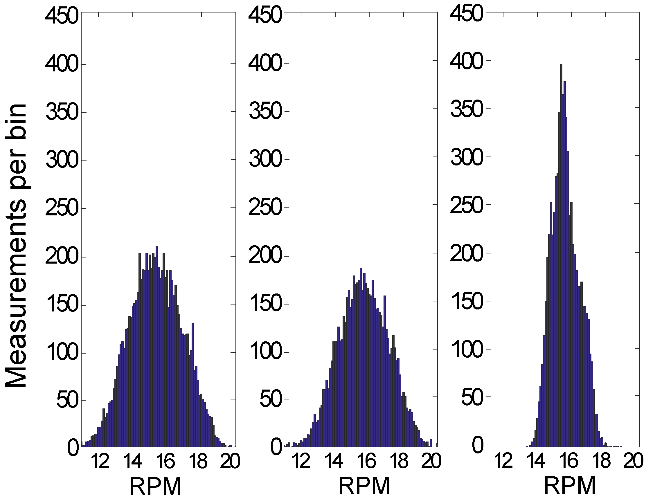
4.3. Rotational Speed Measurements

Figure 9 shows a histogram of the rotational speed and reveals that the DC voltage control was able to reduce the variance in RPM. Table 2 shows calculated average values, variances and the average λ. The average λ was determined for each load case using Equation (3) together with the average RPM and the average water velocity at the turbine. The variance in the constant DC case is reduced by a factor of ∼ 3.5 compared to the AC case.

Figure 9. Histogram of the rotational speed of the turbine during load conditions. From left to right: AC load, fixed PWM and constant DC.

Figure 9. Histogram of the rotational speed of the turbine during load conditions. From left to right: AC load, fixed PWM and constant DC.

Table 2. Rotational speed of the turbine and the number of measurements of the three load cases. Calculated average λ from the average water speed and average RPM.

Load Case	AC	Fixed PWM	Constant DC
Average RPM	15.35	15.68	15.65
Variance	2.34	2.11	0.65
Average λ	3.61	3.65	3.67

Table 2. Rotational speed of the turbine and the number of measurements of the three load cases. Calculated average λ from the average water speed and average RPM.

Load Case	AC	Fixed PWM	Constant DC
Average RPM	15.35	15.68	15.65
Variance	2.34	2.11	0.65
Average λ	3.61	3.65	3.67

A statistical analysis will help to compare the three measured average RPM values. For all three cases, a one-sample Kolmogorov–Smirnov test with a p-value of 0.05 rejects the hypothesis that they come from a normal distribution. A Levene test with a p-value of 0.05 rejects that the variances are equal. A Wilcoxon signed rank test with a p-value of 0.05 cannot reject a zero median in difference in mean values between the fixed PWM case and the constant DC case, but rejects the other two. This means that for all three cases, the RPM measurements have different variances and that the fixed PWM case and the constant DC case have comparable average values.

4.4. Current Measurements

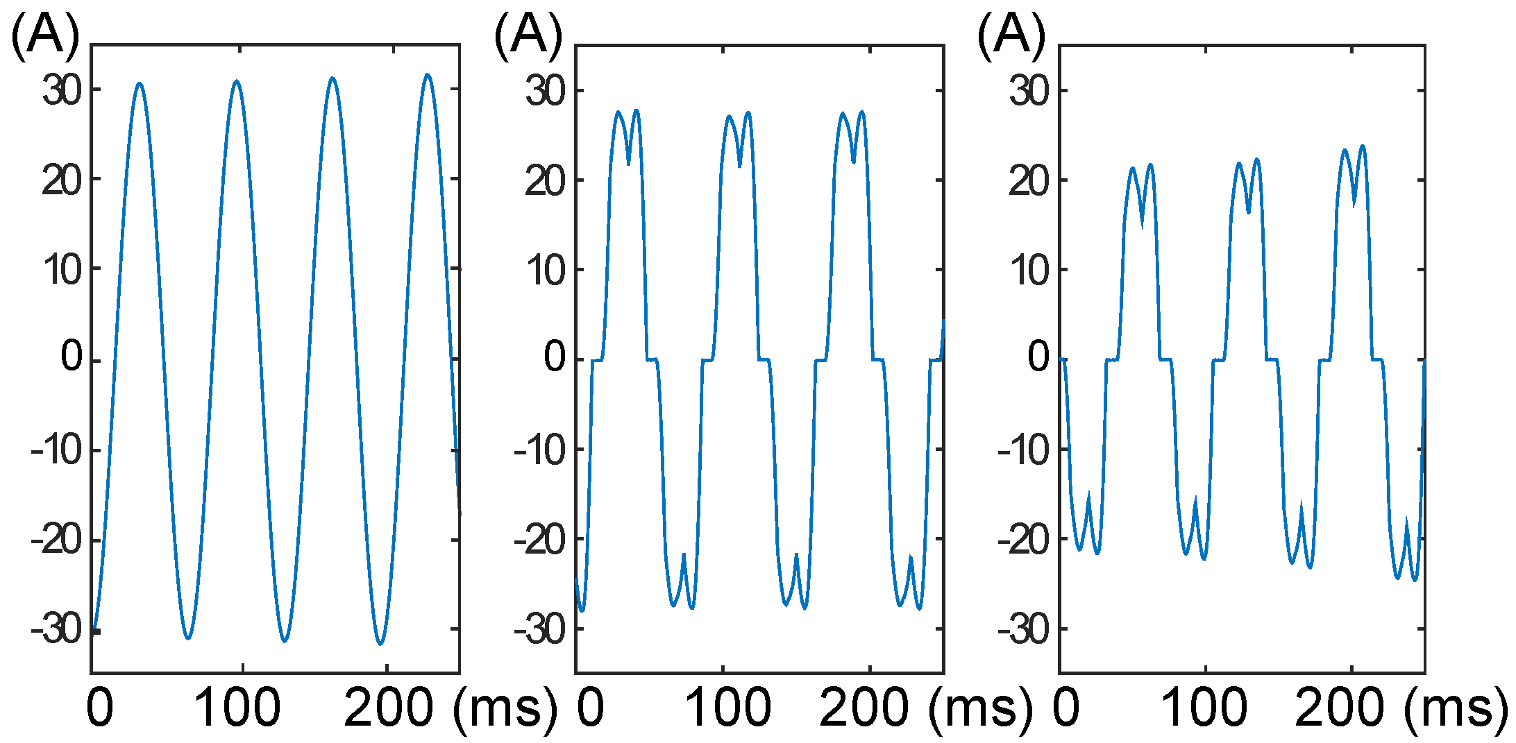
Figure 10 shows the AC currents in one phase for each case. The AC case has the highest amplitude for the current, fixed PWM the second highest and the constant DC case the lowest. The rectifier causes the non-sinusoidal shape of the currents drawn in the fixed PWM and the constant DC cases and results in a higher RMS current, which gives higher losses in the transmission lines and windings. The losses are calculated with Equation (7) and shown in Table 3.

Figure 10. Currents in one phase from the generator. From left to right: AC load, fixed PWM and constant DC.

Figure 10. Currents in one phase from the generator. From left to right: AC load, fixed PWM and constant DC.

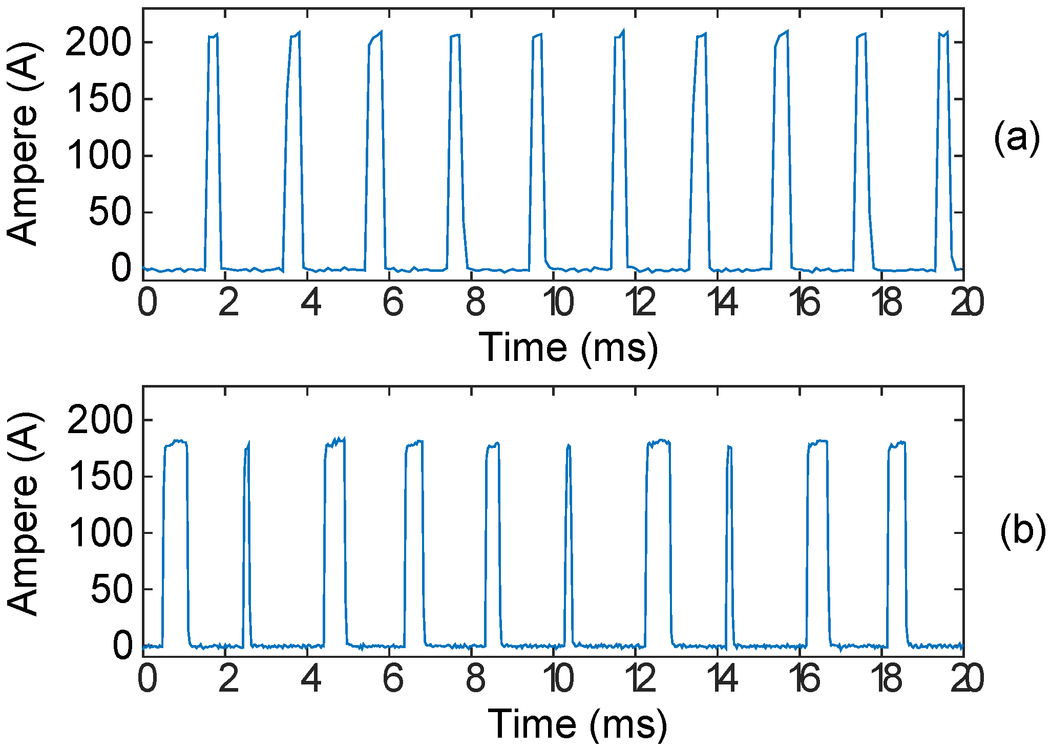
Figure 11 shows the load currents in the DC cases. Figure 11a shows that the duty cycle is constant, and Figure 11b shows that the duty cycle is changing, following the design of the control methods. The difference in amplitude for the currents in Figure 11a,b is roughly 30 A higher (∼ 16% higher) for the fixed PWM case. Even though, as a result of the varying duty cycle in the constant DC case, the average power delivered to the load was merely ∼ 2% higher in the fixed PWM case compared to the constant DC case. The average power calculated using the current and Equation (7) is shown in Table 3.

Figure 11. (a) Current in the load in the fixed PWM case. (b) Current in the load in the constant DC case.

Figure 11. (a) Current in the load in the fixed PWM case. (b) Current in the load in the constant DC case.

Out of the three cases, the losses were the greatest for the constant DC case, both in terms of magnitude and in terms of losses/total electric power delivered; see Table 3.

Table 3 shows measured resistances, calculated RMS phase current in the transmission line, calculated average powers, P_turbine from Table 1 and calculated η_system from Equation (6).

Despite having different size of losses and shapes of currents both drawn from the generator and delivered to the load, η_system was about the same for the three load control methods.

Table 3. Measured resistances, calculated RMS current in each phase, calculated power, P_kinetic (from Table 1), fraction of losses to P_losses + P_load and system efficiency η_system.

Load Case	AC	Fixed PWM	Constant DC
Rload (Ω/phase)	3.52	0.86	0.86
Rlines + Rwindings (Ω/phase)	0.435	0.435	0.435
iRMSphase (A)	20.77	23.23	23.53
Pload (kW)	4.60	4.55	4.44
Plosses (kW)	0.56	0.70	0.72
Plosses + Pload(kW)	5.16	5.26	5.17
Plosses/ (Plosses + Pload) (%)	10.9	13.3	13.9
Mean Pkinetic (kW)	27.44	28.15	27.78
ηsystem	0.188	0.187	0.186

Table 3. Measured resistances, calculated RMS current in each phase, calculated power, P_kinetic (from Table 1), fraction of losses to P_losses + P_load and system efficiency η_system.

Load Case	AC	Fixed PWM	Constant DC
Rload (Ω/phase)	3.52	0.86	0.86
Rlines + Rwindings (Ω/phase)	0.435	0.435	0.435
iRMSphase (A)	20.77	23.23	23.53
Pload (kW)	4.60	4.55	4.44
Plosses (kW)	0.56	0.70	0.72
Plosses + Pload(kW)	5.16	5.26	5.17
Plosses/ (Plosses + Pload) (%)	10.9	13.3	13.9
Mean Pkinetic (kW)	27.44	28.15	27.78
ηsystem	0.188	0.187	0.186

5. Discussion

At λ_opt, the power coefficient is estimated to be 0.36. If the rotational speed of the turbine was kept at λ_opt during the 30 min, it would theoretically result in a maximum 36% average extracted electric power. This number is in reality probably lower, since it does not include the losses in the bearings or the efficiency of the generator.

It is noteworthy that the AC load case without active control had roughly the same η_system as the other two cases. The rectifier and capacitor bank introduces non-linear loads in the electrical circuit. The induced harmonics from the rectification increases the RMS value of the currents drawn from the generator, hence increasing the copper losses in the transmission lines and windings. A common solution to lower the transmission losses would be to increase the voltage over the transmission line with a transformer. This would be difficult to include in the present generator housing design because of lack of space. The design advantage of the AC load case is the lack of electric components that make it inexpensive and require little maintenance. The advantage of the DC control is that it has the potential for MPPT that could increase the average extracted power. If an MPPT were developed, it would be reasonable to believe that the duty cycle will change more and/or more quickly. Both of these things can make the RMS value of the current even higher, and the losses would be higher. Introducing an MPPT will be about weighing the increase of η_system with respect to the increase of P_load/P_turbine.

The authors chose P_turbine ∼ P_losses + P_load in order to include the impact of the length of the transmission lines on η_system. If the losses were not included, η_system would be defined as P_load/P_kinetic, and the results would be 16.8%, 16.2% and 16.0% for the AC, fixed PWM and constant DC cases, respectively. P_turbine ∼ P_losses + P_load was chosen, since this study is supposed to evaluate the system efficiency of how much electric power is extracted with the control methods, not the efficiency to supply a load at a certain distance from the generator and turbine.

The simple P-controller was able to keep the variance of the rotational speed at ∼ 4.2%. This would result in a suitable DC voltage for a grid side converter. An MPPT system will aim to extract maximum power from the river, which means it will adapt the rotational speed of the turbine to the water speed. Hopefully, this adaption of rotational speed will increase the average extracted power without sacrificing the stability of the DC bus voltage. The low variation of the DC bus voltage in this case indicates that there would be no need for additional components to convert the voltage from the generator to manageable limits.

6. Conclusions

The authors feel the reported study warrants the following conclusions. The experimental results indicate that DC bus voltage control is the best suited for marine current applications compared with a fixed PWM or a fixed AC load. The DC bus voltage control system was able to keep the variations of rotational speed by a factor of ∼ 3.5 lower during 30 minutes of operation than the other two cases. The P-controller in the DC bus voltage control was able to keep the variance of the rotational speed at ∼ 4.2%. A PID controller could reduce the variance further at the cost of a potentially more rapidly changing switching frequency of the load IGBT, which may increase the losses from non-linear load even more. The average tip speed ratio for all three cases was close to the estimated λ_opt = 3.5, but resulted in only η_system = ∼ 19%, which is almost half of the predicted theoretical maximum of 36%. An MPPT system should be able to increase η_system.

References

- Apelfröjd, S.; Bülow, F.; Kjellin, J.; Eriksson, S. Laboratory Verification of System for Grid Connection of a 12 kW Variable Speed Wind Turbine with a Permanent Magnet Synchronous Generator. In Proceedings of the EWEA 2012, European Wind Energy Conference & Exhibition, Copenhagen, Denmark, 16–19 April 2012.
- Abbes, M.; Belhadj, J.; Ben Abdelghani Bennani, A. Design and control of a direct drive wind turbine equipped with multilevel converters. Renew. Energy 2010, 35, 936–945. [Google Scholar] [CrossRef]
- Molina, M.G.; Mercado, P.E. A New Control Strategy of Variable Speed Wind Turbine Generator for Three-Phase Grid-Connected Applications. In Proceedings of the 2008 IEEE/PES Transmission and Distribution Conference and Exposition: Latin America, Bogotà, Colombia, 13–15 August 2008.
- Eriksson, S.; Kjellin, J.; Bernhoff, H. Tip speed ratio control of a 200 kW VAWT with synchronous generator and variable DC voltage. Energy Sci. Eng. 2013, 1, 135–143. [Google Scholar] [CrossRef]
- Kjellin, J.; Eriksson, S.; Bernhoff, H. Electric Control Substituting Pitch Control for Large Wind Turbines. J. Wind Energy 2013, 2013, 1–4. [Google Scholar] [CrossRef]
- Thongam, J.S.; Bouchard, P.; Ezzaidi, H.; Ouhrouche, M. Wind Speed Sensorless Maximum Power Point Tracking Control of Variable Speed Wind Energy Conversion Systems. In Proceedings of the 2009 IEEE International Conference on Electric Machines and Drives, Miami, FL, USA, 3–6 May 2009; pp. 1832–1837.
- Haque, M.E.; Negnevitsky, M.; Muttaqi, K.M. A Novel Control Strategy for a Variable Speed Wind Turbine with a Permanent Magnet Synchronous Generator. In Proceedings of the 2008 IEEE Industry Applications Society Annual Meeting, Edmonton, AB, Canada, 5–9 October 2008; pp. 1–8.
- Jeong, H.G.; Seung, R.H.; Lee, K.B. An improved maximum power point tracking method for wind power systems. Energies 2012, 5, 1339–1354. [Google Scholar] [CrossRef]
- Kjellin, J. Vertical Axis Wind Turbines: Electrical System and Experimental Results. Ph.D. Thesis, Uppsala University, Uppsala, Sweden, 30 November 2012. [Google Scholar]
- Lundin, S.; Forslund, J.; Carpman, N.; Grabbe, M.; Yuen, K.; Apelfröjd, S.; Goude, A.; Leijon, M. The Söderfors Project: Experimental Hydrokinetic Power Station Deployment and First Results. In Proceedings of the 10th European Wave and Tidal Energy Conference, EWTEC13, Aalborg, Denmark, 2–5 September 2013.
- Grabbe, M.; Yuen, K.; Goude, A.; Lalander, E.; Leijon, M. Design of an experimental setup for hydro-kinetic energy conversion. Int. J. Hydropower Dams. 2009, 15, 112–116. [Google Scholar]
- Yuen, K.; Lundin, S.; Grabbe, M.; Lalander, E.; Goude, A.; Leijon, M. The Söderfors Project: Construction of an Experimental Hydrokinetic Power Station. In Proceedings of the 9th European Wave and Tidal Energy Conference, EWTEC11, Southampton, UK; 2011; pp. 1–5. [Google Scholar]
- Grabbe, M.; Yuen, K.; Apelfröjd, S.; Leijon, M. Efficiency of a directly driven generator for hydrokinetic energy conversion. Adv. Mech. Eng. 2013, 5. [Google Scholar] [CrossRef]
- Yuen, K.; Apelfröjd, S.; Leijon, M. Implementation of Control System for Hydro-kinetic Energy Converter. J. Control Sci. Eng. 2013, 2013. [Google Scholar] [CrossRef]
© 2015 by the authors; licensee MDPI, Basel, Switzerland. This article is an open access article distributed under the terms and conditions of the Creative Commons Attribution license (http://creativecommons.org/licenses/by/4.0/).