Adaptive Disturbance Observer-Based Parameter-Independent Speed Control of an Uncertain Permanent Magnet Synchronous Machine for Wind Power Generation Applications

Abstract

This paper proposes a parameter-independent speed controller based on the classical cascade speed control strategy comprising an inner-loop current controller and an outer-loop speed controller for permanent magnet synchronous machines. The contribution of this paper is three-fold: the first is the proposal of a parameter-independent current controller in the inner loop with global asymptotic stability guarantee; the second is the presentation of a guideline for choosing stabilizing proportional-integral (PI) gains in the outer loop; and the third is designing an adaptive disturbance observer (ADOB) to predict the one step ahead state, so that this predicted state compensates the one-step time delay on the control input. The effectiveness of the proposed controller is demonstrated by simulating a wind power generation application using powerSIM (PSIM) software.

1. Introduction

Permanent magnet synchronous machines, such as generators (PMSG) and motors (PMSM), are widely used for various electrical/mechanical power generation applications owing to their high efficiency, high power factor and simple structures [1–8].

Conventionally, a cascade control strategy has been used for controlling the speed of synchronous machines. This strategy involves the use of two proportional-integral (PI) controllers for inner loop current control and outer loop speed control [2,3,9]. Because the inner loop current controller plays a crucial role in enhancing closed-loop performance, several current controllers have been reported, such as PI controllers [2,3,9], nonlinear controllers [4,5,10,11] and optimal controllers [12,13]. However, the nonlinear controllers [4,5,10,11] and optimal controllers [12,13] require exact PMSM parameter values, upper and lower bounds of the PMSM parameters or, at least, PMSM parameters generated using a properly-designed parameter estimator. In the case of the PI controllers [2,3,9], although PMSM parameter information is not explicitly used in the controller, the closed-loop poles rely on the PMSM parameters. Dependency on PMSM parameters could limit the closed-loop performance or lead to instability of the closed-loop system, because it is difficult to acquire exact PMSM parameter values, and these values slowly change with the passage of time. Although a suitably-designed parameter estimator can avoid this limitation, the computational burden would increase.

Following the classical cascade control strategy, in this paper, a parameter-independent current controller for the inner loop with global asymptotic stability is proposed, and it is shown that any positive PI gain in the outer loop leads to asymptotic convergence of the PMSG speed with its reference value. The proposed current controller uses only current information and, unlike [4,5,10–13], does not require any PMSG parameter information, even that about the upper and lower bounds of the parameters. Moreover, because the controller structure is very simple, similar to the classical PI controller, its implementation is easy. It is shown that any symmetric and positive-definite control gain leads to the global asymptotic stability of closed-loop systems; this result is in sharp contrast with the results obtained in [2,3,9]. Furthermore, it is proven that an outer loop PI controller with any positive PI gain forces the PMSG speed to track its reference value. In order to compensate the one-step time delay that is inevitable in the real implementation, we design an adaptive disturbance observer (ADOB), so that its predicted state compensates the one-step time delay on the control input. Through the results of simulations using powerSIM (PSIM) software, it is shown that the closed-loop performance of the proposed controller is satisfactory for controlling the speed of a PMSG in wind power generation.

2. PMSG Model in a Rotating d-q Frame

For convenience, a PMSG is considered in the rest of the paper, because the dynamic equations of a PMSG and a PMSM are very similar. The dynamics of the surface-mounted PMSG used herein is described in the rotating d-q frame as follows [9]:

$${\dot{\omega }}_r(t)=-\frac{B_m}{J_m}{\omega }_r(t)+\frac{1}{J_m}(T_m(t)-T_e(\mathbf{x}(t)))$$

(1)

$$\dot{\mathbf{x}}(t)=({\omega }_e(t)\mathbf{J}-\mathbf{R})\mathbf{x}(t)+\mathbf{Bu}(t)-{\omega }_e(t)\mathbf{d},\forall t\ge 0$$

(2)

where B_m and J_m represent the viscous friction and rotor moment of inertia, respectively, and ω_r(t) and T_m(t) denote the rotor speed and mechanical load torque, respectively. The state variable x(t), control input u(t), torque T_e(x(t)) and electric rotational rotor speed ω_e(t) are defined as follows:

$$\mathbf{x}(t)=\left[\begin{array}{l}{x}_1(t)\hfill \\ x_2(t)\hfill \end{array}\right]:=\left[\begin{array}{l}{i}_d(t)\hfill \\ i_q(t)\hfill \end{array}\right],\mathbf{u}(t)=\left[\begin{array}{l}{u}_1(t)\hfill \\ u_2(t)\hfill \end{array}\right]:=\left[\begin{array}{l}{\upsilon }_d(t)\hfill \\ {\upsilon }_q(t)\hfill \end{array}\right]$$

$$T_e(\mathbf{x}(t)):=\frac{3}{2}P{\lambda }_m{x}_2(t),{\omega }_e(t):=P{\omega }_r(t),\forall t\ge 0$$

where P and λ_m denote the number of pole pairs and the permanent magnet flux, respectively. Matrices J, R, B and d are expressed as follows:

$$\mathbf{J}:=\left[\begin{array}{ll}0\hfill & 1\hfill \\ -1\hfill & 0\hfill \end{array}\right],\mathbf{R}:=\frac{R_s}{L}{\mathbf{I}}_{2\times 2},\mathbf{B}:=\left[\begin{array}{ll}\frac{1}{L}\hfill & 0\hfill \\ 0\hfill & \frac{1}{L}\hfill \end{array}\right],\mathbf{d}:=\frac{{\lambda }_m}{L}\left[\begin{array}{l}0\hfill \\ 1\hfill \end{array}\right]$$

where I_2×2 refers to a 2 × 2 dimensional identity matrix and R_s and L are stator resistance and inductance, respectively. Physically, the values of R_s and L should be positive. The next section designs a parameter-independent speed controller under the classical cascade speed control strategy using the state Equation (2).

3. Controller Design

This section presents a cascade speed control scheme without any use of parameter information of the PMSM, considering the one-step time delay on the control input. Section 3.1 constructs a parameter-independent current controller for the inner-loop, so that the current asymptotically converges to its reference. Section 3.2 describes how to assign the stabilizing control gain of the outer-loop PI controller. Section 3.3 designs an ADOB in order to predict the one-step ahead state, so that it makes up for the one-step time delay on the control input that is inevitable in the real implementation.

3.1. Parameter-Independent Current Controller Design and Stability Analysis

This section describes the construction of a parameter-independent current controller for achieving the control objective:

$$\underset{t\to \infty }{\lim }\mathbf{x}(t)=\mathbf{r}$$

(3)

where $r={\left[\begin{array}{ll}{r}_d\hfill & r_q\hfill \end{array}\right]}^T$ denotes a current reference. Then, the following current controller is proposed:

$$\mathbf{u}(t)=-{\mathbf{K}}_1\mathbf{x}(t)-{\mathbf{K}}_2\mathbf{z}(t)$$

(4)

$$\dot{\mathbf{z}}(t)={\mathbf{e}}_x(t),\forall t\ge 0$$

(5)

where K₁ ∈ ℝ^2×2 and K₂ ∈ ℝ^2×2 are the controller gain matrices, and the tracking error e_x(t) is defined as e_x(t) := x(t) − r, ∀t ≥ 0. It is observed that the proposed controller comprising Equations (4) and (5) is very simple, similar to the classical PI controller, as well as completely independent of the PMSG parameters. The closed-loop stability can be proven by imposing a constraint on the controller gains K₁ and K₂. For details, see Theorem 1. The mechanical dynamics of most electrical machines is much slower than their electrical dynamics. Therefore, when considering only the electrical state Equation (2), it makes sense to assume that there exist an unknown constant ${\omega }_e^0$ and a sequence (a₀, a₁, ⋯, a_n−1), such that the ordinary differential equation:

$${\tilde{\omega }}_e^{(n)}(t)+a_{n-1}{\tilde{\omega }}_e^{(n-1)}(t)+\cdots +a_1{\dot{\tilde{\omega }}}_e(t)+a_0{\tilde{\omega }}_e(t)=0,\forall t\ge 0$$

(6)

is stable, which means that the all roots of Equation (6) are placed in the left half plane of the complex number space. Here, the speed error ῶ_e(t) is defined as ${\tilde{\omega }}_e(t):={\omega }_e(t)-{\omega }_e^0$, i.e., ω_e(t) is time-varying, but exponentially converges to an unknown constant ${\omega }_e^0$ as time goes by.

Theorem 1. Suppose that there exists a sequence (a₀, a₁, ⋯, a_n−1, a_n), such that Equation (6) is stable and that the matrices K₁ and K₂ in the controller (4)–(5) are chosen to be symmetric and positive-definite, i.e.,

$${\mathbf{K}}_1={\mathbf{K}}_1^T>0,{\mathbf{K}}_2={\mathbf{K}}_2^T>0.$$

(7)

Then, the closed-loop system comprising the state equation (2) and the proposed controller (4)–(5) is globally asymptotically stable.

From the result of Theorem 1, it is seen that the proposed controller (4)–(5) with the control gain satisfying Condition (7) establishes the control objective (3). Furthermore, the proposed controller does not depend on the PMSG parameters, and the closed-loop stability is preserved as long as the values of all parameters are positive, unlike those of [2,3,9].

3.2. ADOB Design for Time Delay Compensation

The Euler approximation makes it possible to implement the differential operator in such a way that:

$$\dot{f}(t)\approx \frac{f(t+h)-f(t)}{h},\forall t,h>0$$

where f denotes a given differentiable function. According to this relation, the proposed controller (4)–(5) must be implemented as:

$$\mathbf{u}(k)=-{\mathbf{K}}_1\mathbf{x}(k)-{\mathbf{K}}_2\mathbf{z}(k)$$

(8)

$$\mathbf{z}(k+1)=\mathbf{z}(k)+h{\mathbf{e}}_x(k),\forall k\ge 0$$

(9)

where h denotes the sampling period, and e_x(k) := x(k) − r. Because the one-step time delay on the control input is inevitable in the real implementation using a micro-processor, it is impossible to implement the controller (4)–(5) in the form of Equations (8)–(9). The proposed control law Equations (4)–(5) will be implemented as:

$$\mathbf{u}(k)=-{\mathbf{K}}_1\mathbf{x}(k-1)-{\mathbf{K}}_2\mathbf{z}(k-1)$$

(10)

$$\mathbf{z}(k)=\mathbf{z}(k-1)+h{\mathbf{e}}_x(k-1),\forall k\ge 0$$

(11)

Because this one-step time delay on the control input may make the closed-loop performance degraded or even unstable, it must be compensated. This paper proposes an adaptive disturbance observer (ADOB) for compensating the the one-step time delay as follows:

$$\dot{\widehat{\mathbf{x}}}(t)={\omega }_e(t)\mathbf{Jx}(t)-{\widehat{\theta }}_1\mathbf{x}(t)+{\widehat{\theta }}_2\mathbf{u}(t)-{\omega }_e(t)\widehat{\mathbf{d}}(t)+{\mathbf{L}}_1{\mathbf{e}}_o(t)$$

(12)

$$\dot{\widehat{\mathbf{d}}}(t)=-{\mathbf{L}}_2{\omega }_e(t){\mathbf{e}}_o(t)$$

(13)

$${\dot{\widehat{\theta }}}_1(t)=-{\gamma }_1{\mathbf{x}}^T(t){\mathbf{e}}_o(t)$$

(14)

$${\dot{\widehat{\theta }}}_2(t)={\gamma }_2{\mathbf{u}}^T(t){\mathbf{e}}_o(t),\forall t\ge 0$$

(15)

where e_o(t) denotes the state estimation error defined as ${\mathbf{e}}_o(t)=\mathbf{x}(t)-\widehat{\mathbf{x}}(t)$,∀t ≥ 0, L₁ ∈ ℝ^2×2, L₂ ∈ ℝ^2×2, γ₁ and γ₂ are estimation gains to be used as design parameters and δ_d, δ₁ and δ₂ are small positive constants to be set as small as possible. Because the differential operation on the estimated state $\widehat{\mathbf{x}}(t)$ is implemented as:

$$\dot{\widehat{\mathbf{x}}}(t)\approx \frac{\widehat{\mathbf{x}}(t+h)-\widehat{\mathbf{x}}(t)}{h},\forall t,h>0$$

where h denotes the sampling period, it is seen that the proposed ADOB comprising Equations (12)–(15) can be used as a state predictor generating $\widehat{\mathbf{x}}(k+1)$ if it ensures driving the state estimation error e_o(t) to zero. Theorem 2 proves that the state estimation error e_o(t) is asymptotic towards zero by the proposed ADOB.

Theorem 2. The proposed ADOB comprising Equations (12)–(15) ensures making the corresponding estimation error dynamics globally ultimately bounded for any${\mathbf{L}}_1={\mathbf{L}}_1^T>0$, ${\mathbf{L}}_2={\mathbf{L}}_2^T>0$, γ₁ > 0, γ₂ > 0.

It is observed that the proposed ADOB guarantees a satisfactory asymptotic state estimation performance with a sufficiently small δ_d, as long as L₂ is invertible, because, in the steady state, Equation (13) satisfies that:

$${\omega }_e^0{\mathbf{L}}_2{\mathbf{e}}_o^0\approx 0$$

where ${\mathbf{e}}_o^0$ is the steady-state value of e_o(t).

Because it is possible to feedback the one step ahead predicted state $\widehat{\mathbf{x}}(k+1)$ thanks to the ADOB equations (12)–(15), it is possible to implement the proposed control law (4)–(5) as follows:

$$\mathbf{u}(k)=-{\mathbf{K}}_1\widehat{\mathbf{x}}(k)-{\mathbf{K}}_2\mathbf{z}(k)$$

(16)

$$\mathbf{z}(k+1)=\mathbf{z}(k)+h{\widehat{\mathbf{e}}}_x(k),\forall k\ge 0$$

(17)

where ${\widehat{\mathbf{e}}}_x(k):=\widehat{\mathbf{x}}(k)-\mathbf{r},\forall k\ge 0$.

3.3. Speed Controller Design in the Outer Loop

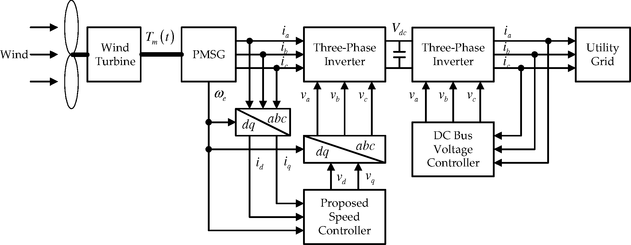
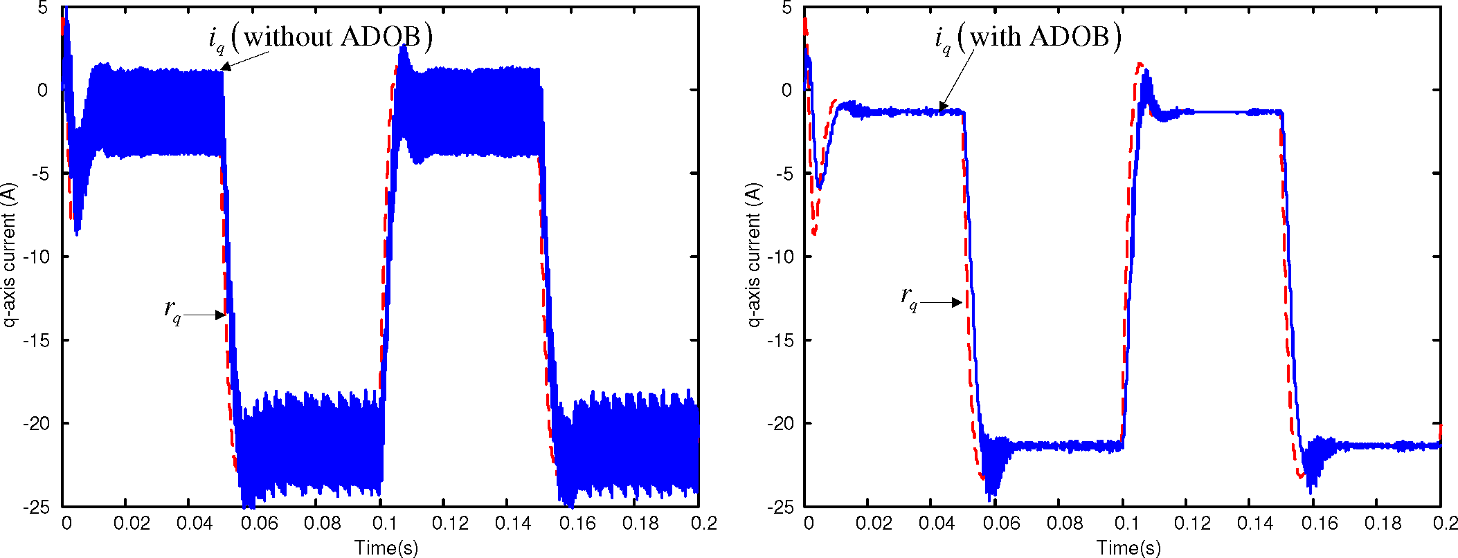
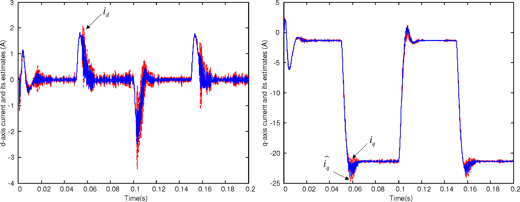
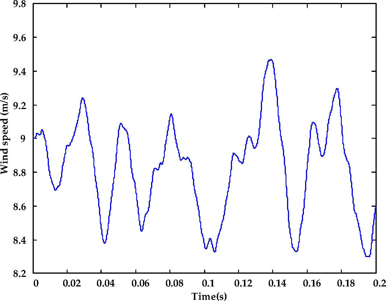
This section presents a guideline for choosing PI gains in the outer loop, such that the PMSG speed is forced to track its reference value for any positive PI gain in the presence of PMSG parameter uncertainties. To this end, we consider that the inner-loop control system with the proposed controller is sufficiently fast and assume that:

$$i_q(t)\approx r_q(t),\forall t\ge 0$$

(18)

where r_q(t) is a signal that varies slowly with time. Note that this type of assumption is also made in [14,15]. Let signal r_q(t) be the output of the outer-loop PI controller as follows:

$$r_q(t)=k_P{e}_{\omega }(t)+k_I{\displaystyle {\int }_0^t{e}_{\omega }(\tau )d\tau ,\forall t\ge 0}$$

(19)

where $e_{{\omega }_r}(t):={\omega }_r(t)-r$, ∀t ≥ 0 and r denotes a speed reference. Then, through some algebraic manipulations after substituting Equation (1) into Equation (19) under the assumption in Equation (18), it can be verified that:

$${\ddot{e}}_{{\omega }_r}(t)+c_1(k_P){\dot{e}}_{{\omega }_r}(t)+c_o(k_I)e_{{\omega }_r}(t)=\frac{1}{J_m}{\dot{T}}_m(t),\forall t\ge 0$$

(20)

where:

$$\begin{array}{l}{c}_1(k_P):=\frac{3P{\lambda }_m}{2J}{k}_P+\frac{B_m}{J_m}\\ c_0(k_I):=\frac{3P{\lambda }_m}{2J_m}{k}_I\end{array}$$

Because the coefficients c₁(k_P) and c₀(k_I) are positive for any k_P > 0 and k_I > 0, the ordinary differential equation (20) indicates that the speed error $e_{{\omega }_r}(t)$ converges to zero for any positive PI gain given that the mechanical torque T_m(t) is sufficiently slow, so that ${\dot{T}}_m(t)=0$, ∀t. That is,

$$\underset{t\to \infty }{\lim }{e}_{{\omega }_r}(t)=0,\forall k_P>0,\forall k_I>0,\forall e_{{\omega }_r}(0)$$

(21)

Although the mechanical load torque satisfies ${\dot{T}}_m(t)=d(t)$, ∀t, for some unknown norm-bounded signal d(t), it can be proven that any positive PI gain guarantees that the speed error is ultimately bounded. That is,

$$\underset{t\to \infty }{\lim }|e_{{\omega }_r}(t)|\le \delta (\overline{d}),\forall k_P>0,\forall k_I>0,\forall e_{{\omega }_r}(0)$$

(22)

where $\delta (\overline{d})$ is a positive constant and the constant $\overline{d}$ satisfies $|d(t)|\le \overline{d}$, ∀t. Here, it is reasonable to assume that ${\dot{T}}_m(t)=d(t)$, ∀t, for the wind power generation application. This analysis is justified if the inner loop control system is sufficiently fast, so that signal r_q(t) generated by the outer loop PI controller can be treated as a constant.

4. Simulations

In this section, we simulate a PMSG-based wind power generation system using PSIM software, as shown in Figure 1. The PMSG speed is controlled by the proposed controller; the DC link voltage V_dc is regulated to the value 600 V by the classical PI controller; and the capacitor value of the DC link voltage is given as C = 1000 μF. The wind turbine part is emulated using the wind turbine block of the renewable energy package in the PSIM software where the nominal output power, moment of inertia, base wind speed, base rotational speed and initial rotational speed are set to be 1 kW, 1 × 10⁻³ kgm², 12 m/s, 50 rpm and 10 rpm, respectively.

The PMSG parameters are given by:

$$\begin{array}{c}{R}_s=5\mathrm{\Omega },L=10\mathrm{mH},{\lambda }_m=0.11307\mathrm{Wb},P=3,\\ J_m=0.0046{\mathrm{kg}\mathrm{m}}^2,B_m=0.1\mathrm{Nm}/\mathrm{rad}/\mathrm{s}.\end{array}$$

Space vector pulse width modulation (SVPWM) is used for implementing the proposed controller, and its period is set to 0.1 ms. As shown in Figure 2, the proposed controller is implemented with the sampling period h = 0.1 ms where the one-step time delay elements are used for the realistic simulation.

Because it is assumed that all PMSG parameters are uncertain, the controller gain should be adjusted using an ad hoc method. A control gain tuning guideline is summarized as follows:

• Connect a constant speed load to the PMSG for fixing the speed using the secondary inverter, and set all control gains to zero.
• Choose the inner-loop proportional gain matrix ${\mathbf{K}}_1={\mathbf{K}}_1^T>0$, such that the d-q frame current tends to a value as quickly as possible without overshoot.
• Choose the inner-loop integral gain matrix ${\mathbf{K}}_2={\mathbf{K}}_2^T>0$, such that the d-q frame’s current converges as quickly as possible to its reference value without overshooting it.
• Remove the constant-speed load connected to the PMSG.
• Choose the outer-loop proportional gain k_P, such that the speed approaches its reference value as soon as possible without overshooting it.
• Choose the outer-loop integral gain k_I, such that the speed converges to its reference value as quickly as possible without overshooting it.

Thus, the controller gains are tuned as follows:

$${\mathbf{K}}_1=\left[\begin{array}{cc}150& 50\\ 50& 150\end{array}\right],{\mathbf{K}}_2=\left[\begin{array}{cc}{10}^5& 3000\\ 3000& {10}^5\end{array}\right]$$

k_P = 0.05, and k_I = 300. The current reference is set to $\mathbf{r}={\left[\begin{array}{ll}{r}_d\hfill & r_q\hfill \end{array}\right]}^T={\left[\begin{array}{ll}0\hfill & r_q(t)\hfill \end{array}\right]}^T$, where r_q(t) denotes the output signal generated by the PI controller (19). Note that, for orienting all linkage flux along the d-axis and maximizing the torque per ampere, the d-frame current must be regulated to zero [16,17]. Thus, we set r_d = 0. The parameters of ADOB of Equations (12)–(15) are tuned as:

$${\mathbf{L}}_1={\mathbf{L}}_2=5000{\mathbf{I}}_{2\times 2},{\gamma }_1=1500,{\gamma }_2=1500$$

so that the state estimation error goes to zero as quickly as possible.

It is assumed that the speed reference r is given as a square wave with the minimum and maximum speeds of 45 rpm and 70 rpm, respectively. First, we assume that a constant wind speed of 9 m/s is applied to the wind power generation system shown in Figure 1. This means that the PMSG is subjected to a constant load torque. Figures 3–5 show that the proposed current controller successfully forces the current and the PMSM speed to their references, and the ADOB keeps the ripples in the current and the speed considerably small despite the one-step time delay on the control input. Moreover, these results also show that the selected PI gain ensures the convergence of the PMSG speed under a constant load torque; i.e., the property in Equation (21) is established.

Figure 6 shows that the current estimation performance of the proposed ADOB is satisfactory. Thus, it is expected that the ADOB successfully compensates the one-step time delay on the control input as intended.

Second, we performed a simulation under the scenario that the wind generated using a Weibull distribution-based wind model [18] depicted in Figure 7 is applied to the wind power generation system. Figures 8 and 9 show that the proposed controller successfully drives the current close to its reference value in the presence of load torque variations. Figure 10 shows that the selected PI gain forces the PMSG speed to track its reference value and to be close to the reference value in the presence of random load torque changes; i.e., the property in Equation (22) is achieved. From these results, the ADOB also successfully maintains a satisfactory closed-loop performance by suppressing the ripples in the current and the speed.

Figure 11 shows that the ADOB still provides a satisfactory state estimation performance in the presence of the load torque changes.

5. Conclusions

This paper proposes a parameter-independent speed control scheme for a PMSG under the classical cascade speed control strategy, taking the one-step time delay on the control input into account. The developed controller for the inner loop is as simple as the classical PI controller; therefore, it is easy to implement. Moreover, it is shown that the resulting closed-loop current control system is globally asymptotically stable, so long as the controller gains are chosen to be symmetric and positive definite. In addition, it is proven that any positive PI gain leads to convergence of the PMSG speed with its reference value, and an ADOB is designed to predict the one step ahead state, so that the proposed controller, including the predicted state, efficiently keeps the closed-loop performance satisfactory despite the one-step time delay on the control input. It is shown that, conducting realistic simulations using the PSIM software, the proposed speed controller makes the closed-loop performance satisfactory despite the time-varying disturbance originating from the wind turbine, as well as the one-step time delay on the control input.

References

1. Zhong, L.; Rahman, M.; Hu, W.; Lim, K. Analysis of direct torque control in permanent magnet synchronous motor drives. IEEE Trans. Power Electron. 1997, 12, 528–536. [Google Scholar]
2. Andeescu, G.D.; Pitic, C.; Blaabjerg, F.; Boldea, I. Combined flux observer with signal injection enhancement for wide speed range sensorless direct torque control of IPMSM drives. IEEE Trans. Energy Convers. 2008, 23, 393–402. [Google Scholar]
3. Tang, L.; Zhong, L.; Rahman, M.; Hu, Y. A novel direct torque control for interior permanent-magnet synchronous machine drive with low ripple in torque and flux–A speed-senseroless approach. IEEE Trans. Ind. Appl. 2003, 39, 1748–1756. [Google Scholar]
4. Boldea, I.; Blaabjerg, F. Direct torque control via feedback linearization for permanent magnet synchronous motor drives, Proceedings of the 13th International Conference on Optimization of Electrical and Electronic Equipment (OPTIM), Brasov, Romania, 22–24 May 2012.
5. Fazeli, S.; Zarchi, H.; Soltani, J.; Ping, H. Adaptive sliding mode speed control of surface permanent magnet synchronous motor using input output feedback linearization, Proceedings of the ICEMS, Wuhan, China, 17–20 October 2008.
6. Bae, B.H.; Sul, S.K.; Kwon, J.H.; Byeon, J.S. Implementation of sensorless vector control for super high speed PMSM of turbo compressor. IEEE Trans. Ind. Appl. 2003, 39, 811–818. [Google Scholar]
7. Zhou, J.; Wang, Y. Real-time nonlinear adaptive backstepping speed control for a PM synchronous motor. Control Eng. Pract. 2005, 13, 1259–1269. [Google Scholar]
8. Goudarzi, N.; Zhu, W. A review on the development of wind turbine generators across the world. Int. J. Dyn. Control. 2013, 1, 192–202. [Google Scholar]
9. Krause, P.C.; Wasynczuk, O.; Sudhoff, S. Analysis of Electric Machinery; IEEE Press: Baltimore, MD, USA, 1995. [Google Scholar]
10. Lascu, C.; Boldea, I.; Blaabjerg, F. Direct torque control of sensorless induction motor drives: A sliding-mode approach. IEEE Trans. Ind. Appl. 2004, 40, 582–590. [Google Scholar]
11. Lee, J.; Choi, C.; Seok, J.; Lorenz, R. Deadbeat direct torque control and flux control of interior PMSM with discrete time stator current and stator flux linkage observer. IEEE Trans. Ind. Appl. 2011, 47, 1749–1758. [Google Scholar]
12. Mino-Aguilar, G.; Dominguez, A.M.; Maya, R.; Alvarez, R.; Cortez, L.; Munoz, G.; Guerrero, F.; Maya, S.; Rodriguez, A.M.; Portillo, F.; et al. A Direct torque control for a PMSM, Proceedings of the 20th Electronics, Communications and Computer (CONIELECOMP) 2010, Cholula, Mexico, 22–24 February 2010.
13. Rodriguez, J.; Cortes, P. Predictive control of permanent magnet synchronous motors. Predict. Control. Power Convert. Electr. Drives 2012, 59, 125–138. [Google Scholar]
14. Lee, T.S. Input-output linearization and zero-dynamics control of three-phase AC/DC voltage-source converters. IEEE Trans. Power Electron. 2003, 18, 11–22. [Google Scholar]
15. Lee, T.S. Lagrangian modeling and passivity-based control of three-phase AC/DC voltage-source converters. IEEE Trans. Ind. Electron. 2004, 51, 892–902. [Google Scholar]
16. Kadjoudj, M.; Benbouzid, M.E.H.; Ghennai, C.; Diallo, D. A robust hybrid current control for permanent magnet synchronous motor drive. IEEE Trans. Energy Convers. 2004, 19, 109–115. [Google Scholar]
17. Ke, S.S.; Lin, J.S. Sensorless speed tracking control with backstepping design scheme for permanent magnet synchronous motors, Proceedings of the 2005 IEEE Conference on Control Applications, Toronto, ON, Canada, 28–31 August 2005.
18. Mathew, S. Wind Energy: Fundamentals, Resource Analysis and Economics; Springer: New York, NY, USA, 2006. [Google Scholar]
19. Khalil, H.K. Nonlinear Systems; Prentice Hall: Englewood Cliffs, NJ, USA, 2002. [Google Scholar]
Figure 1. Simulated closed-loop system.
Energies 08 04496f1
Figure 2. Simulated closed-loop system.
Energies 08 04496f2
Figure 3. (Left) d-frame current response without the adaptive disturbance observer (ADOB); (Right) d-frame current response with ADOB.
Energies 08 04496f3
Figure 4. (Left) q-frame current response without ADOB; (Right) q-frame current response with ADOB.
Energies 08 04496f4
Figure 5. (Left) Permanent magnet synchronous motor (PMSM) speed response without ADOB; (Right) PMSM speed response with ADOB.
Energies 08 04496f5
Figure 6. (Left) d-frame current reference estimation performance; (Right) q-frame current reference estimation performance
Energies 08 04496f6
Figure 7. Weibull distribution-based wind model [18].
Energies 08 04496f7
Figure 8. (Left) d-frame current response without ADOB; (Right) d-frame current response with ADOB.
Energies 08 04496f8
Figure 9. (Left) q-frame current response without ADOB; (Right) q-frame current response with ADOB.
Energies 08 04496f9
Figure 10. (Left) PMSM speed response without ADOB; (Right) PMSM speed response with ADOB.
Energies 08 04496f10
Figure 11. (Left) d-frame current reference estimation performance; (Right) q-frame current reference estimation performance
Energies 08 04496f11