1. Introduction
Current high electricity loads require appropriate and adequate power generation. However, it is well known that conventional power generation by means of fossil fuels is a major cause of environmental pollution [
1]. Any comparison of solar energy and conventional generation is unfair if it does not include the indirect costs of conventional energy, which are defined by factors such as its environmental and health impacts [
2]. Solar Thermal Power Plants (STPP) are expected to share the energy production scenario with conventional energy generation technologies like fossil and nuclear [
3].
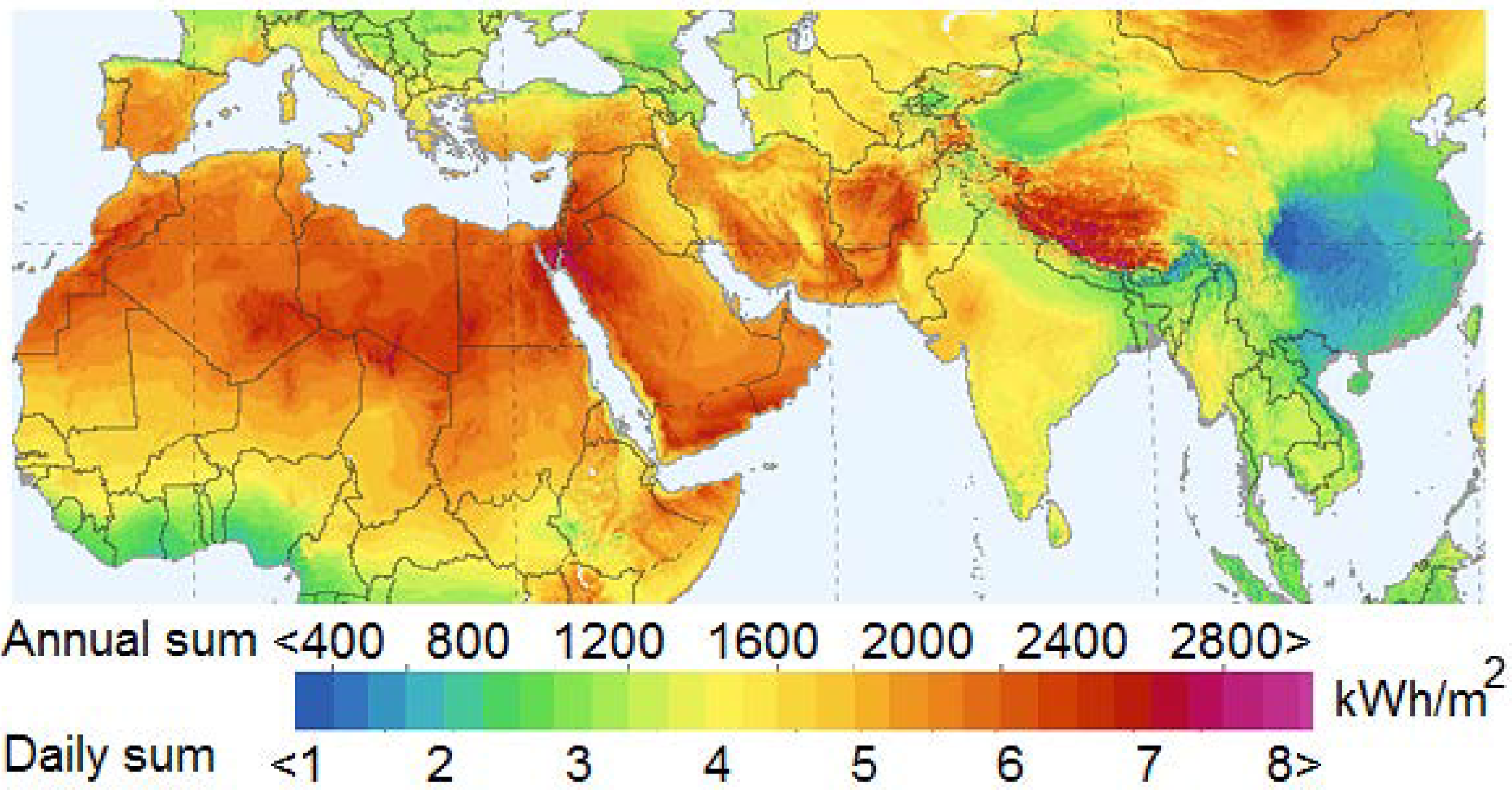
The Middle East, Arabia and the Gulf countries have very high solar radiation potential, especially for direct solar radiation or Direct Normal Irradiance (DNI),
i.e., the fraction of solar radiation which is not deviated by clouds, fumes or dust in the atmosphere and that reaches the Earth’s surface as a parallel beam [
4]. The regional DNI map is shown in
Figure 1. The large area combined with the abundant solar resources has made this region one of the most promising areas for the installation of solar energy plants for providing electricity [
5]. Rural electrification is a global challenge in developing countries, especially those whose area is huge and have a low population in scattered communities or tribes as is the case in most countries of the mentioned region. It also determines the living standard of the people and as well stops the immigration to urban areas [
6].
Figure 1.
Solar radiation distribution over the Middle East, Arabia and Gulf region.
Figure 1.
Solar radiation distribution over the Middle East, Arabia and Gulf region.
Concentration of solar radiation becomes necessary when high temperatures are desired. The concentration ratio is defined as [
7]:
Solar concentrators work perfectly at locations where DNI dominates. Electrical power is produced when the concentrated light is converted into heat, which drives a steam turbine that is connected to an electrical power generator [
8].
Solar radiation is converted into thermal energy in the focus zone of solar thermal concentrating systems. A receiver tube is installed in the focal line with a fluid flowing inside it that absorbs concentrated solar energy from the tube walls and raises its enthalpy. The collector is provided with a one-axis solar tracking system to ensure that the solar beam falls parallel to its axis. Using evacuated tubular absorbers is one of the foremost technologies currently used in solar thermal electric power generation plants [
9].
Previous research work has investigated the thermal performance of parabolic trough collectors for operation with synthetic oil and water as the working fluids. Also, a model of thermal losses from the collector has been developed to predict the performance of the collector with any working fluid. The effects of absorber emissivity and internal working fluid convection effects are evaluated in [
9]. The collector thermal loss when using synthetic oil as the working fluid was estimated to be higher than when using water.
A modelling program called PTCDES was used in the past to predict the quantity of steam produced by the system [
10]. The values of solar radiation and ambient air temperature used in this modelled performance of the system were 500 W/m
2 and 30 °C, respectively.
A Computational Fluid Dynamics (CFD) model has been generated using same software used in this work applied to a North–South oriented solar collectors’ loop, composed of 11 parabolic-trough collector units connected in series, with a total length of 500 m. The experimental test facility is located at the Plataforma Solar de Almería, Spain. The research concluded that the model shows a very good performance and the results presented support the applicability of CFD modeling to study dynamics of direct steam generation in parabolic-trough solar collectors [
11].
A parabolic solar concentrator prototype has been built by other researchers [
12,
13]. Temperatures above 200 °C and pressures up to 12 kg/cm
2 could be achieved experimentally. Higher temperature and pressure could have been achieved, but errors associated with the shape of the parabolic surface existed [
12,
13].
In this work, we propose a standalone portable system comprising a parabolic trough concentrator and a pipe—with flowing water—set in the concentrator’s focus as shown in
Figure 2. As the water flows inside the pipe, the concentrated solar energy is absorbed and steam is generated at the pipe outlet which will in turn drive a steam turbine to generate electricity.
Figure 2.
Flow diagram of the proposed system [
14].
Figure 2.
Flow diagram of the proposed system [
14].
Understanding of the dynamic behavior of the direct steam generation process is essential for proper operation and output optimization of this type of proposed standalone solar plant. Accurate CFD modeling can lead to clear determination of the optimal operating point in the design of such a system, allowing us to identify critical process conditions that may lead to anticipated failures like two-phase flow phenomena occurring in the proposed system.
The aim of the work is to investigate the capability of steam generation using a 1 meter portable parabolic solar concentrator that could operate in remote areas. The study approach is to perform a CFD simulation of water flowing inside the pipe with the relevant physical conditions applied to it like solar radiation intensity, ambient temperature, tube diameter and water flow rate, in order to investigate the quantity and quality of the generated steam.
2. CFD Simulation Approach
Since the outer tube is completely isolated from the inner tube, radiative and conductive heat losses from the outer surface of the inner (metallic) tube are neglected. Rather an overall loss from the inner tube of about 20% is assumed [
15]. Radiative and conductive heat transfer losses from the whole system are considered when we discuss a specific design of a system with known dimensions and materials. Detailed analysis of the heat transfer to water through the evacuated tube is calculated by employing a finite volume algorithm using STAR CCM, a commercially available CFD package that has been tested [
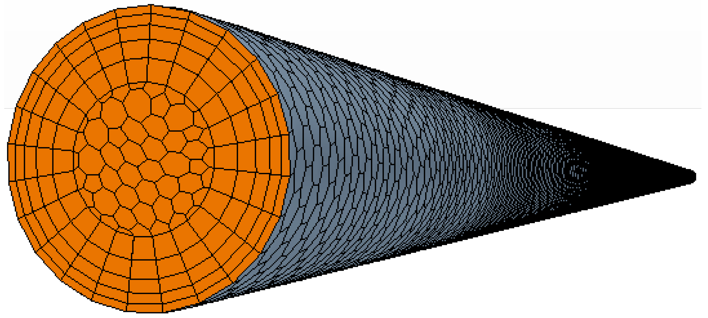
16] and proven good capability for solving such problems. The flowing water has only been taken into consideration in the simulation process with heat loss of about 20% of the incident concentrated solar radiation. Mesh has been built for the 1 m length water using multilayer polyhedral cells as shown in
Figure 3.
Figure 3.
Polyhedral meshing of the water inside the tube.
Figure 3.
Polyhedral meshing of the water inside the tube.
In order to make sure that simulation results are independent of the mesh, a grid sensitivity study with different base-size and growth-rate meshes has been performed applying the physical parameters and boundary conditions listed in
Table 1. Two mesh dimensions have been applied to the tube and resulted in the same solution features as listed in
Table 2. A reduction of the base mesh size from 0.01 m to 0.003 m with a simultaneous increase of number of prism layers has resulted in an increase of the number of volume mesh cells from 156,356 to 233,441. As listed in the Table, a small variation of average outlet temperature (from 479 K in the first set of mesh settings to 486 K in the second mesh) has been found. However, no variations have been observed in the average outlet steam fraction as will be discussed later. The coarser mesh model “Mesh 1” was then adopted, as a good compromise between reasonable grid-independence of the solution and computation time.
A three-dimensional, steady state multiphase fluid model with turbulent flow has been used in the CFD simulation process. In more detail, a single continuity equation (Equation (2)) is solved for a fluid having a mixture of liquid and gas phases, where each distinct phase has its own set of conservation equations.
Phases are considered to be mixed on length scales smaller than the length scales to resolve, and coexist everywhere in the flow domain. The volume fraction is the portion of a volume that a phase occupies [
16,
17,
18].
Table 1.
Dimensions and material of the proposed system.
Table 1.
Dimensions and material of the proposed system.
| Part | Dimensions |
|---|
| Parabolic trough | Length: 1 m
Aperture: 1.6 m
Optical collection efficiency: 64% [10] |
| Evacuated tube | Length: 1 m
Inner tube material: steel
Outer tube material: evacuated glass
Collection efficiency: 80% [15]
Inner tube diameter: 0.005 m, 0.01 m |
| Flowing liquid | Material: Water
Flow rate (kg/h): 0.0019, 0.0022, 0.0025, 0.0028, 0.0031 and 0.0042 |
Table 2.
Mesh specifications used in grid sensitivity test.
Table 2.
Mesh specifications used in grid sensitivity test.
| | Cell base size | No. of prism layers | No. of mesh cells | Ave. outlet temperature (K) | Ave. outlet steam fraction (%) |
|---|
| Mesh 1 | 0.01 m | 5 | 156356 | 479 | 0.98 |
| Mesh 2 | 0.0030 m | 7 | 233441 | 486 | 0.98 |
In addition, the volume fractions must satisfy Equation (3):
In these simulations the realizable two-layer turbulence model [
17] was used. In this model,
Cµ, a critical coefficient of the model, is expressed as a function of mean flow and turbulence properties, rather than assumed to be constant as in the standard model. This allows the model to satisfy certain mathematical constraints of the normal stresses consistent with the physics of turbulence (realizability), which are also consistent with experimental observations in boundary layers. The realizable model is substantially better than the standard model and is implemented in STAR-CCM with a two layer approach, which enables it to be used with fine meshes that resolve the viscous sub-layer. The turbulent viscosity
µt is expressed as [
16,
17]:
where
Cµ is a coefficient given by
,
ρ is the density;
U(*) is a function of strain rate tensor and vorticity tensor;
A0 whose value is taken as 4.0; while
As is taken as [
17,
18]:
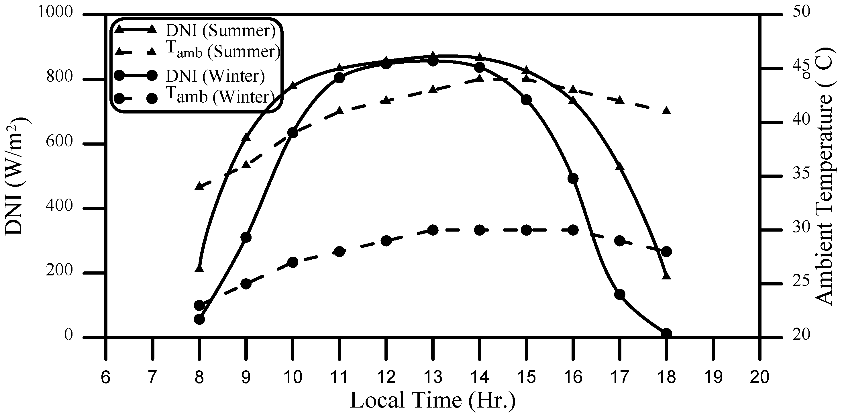
Hourly profiles of direct solar radiation of two selected clear-sky days, representing summer and winter, respectively, along with their ambient temperature values, have been considered, as shown in
Figure 4. The location considered in this paper is Makkah, Saudi Arabia (21.4167° N, 39.8167° E), where the authors reside. These temperature values are used as inputs to the simulation process to calculate the net thermal energy gain of the system. The water inlet’s temperature is assumed as the ambient temperature. Wind speed data was not available for the chosen location, so rather a total loss has been considered.
Figure 4.
Hourly direct solar radiation and ambient temperature profiles for two typical days in summer and winter.
Figure 4.
Hourly direct solar radiation and ambient temperature profiles for two typical days in summer and winter.
3. Simulation Results
Data collected from the CFD simulation are in the form of temperature, volume fractions of water and steam, and velocity of flow of the fluid components at almost every point inside the tube.
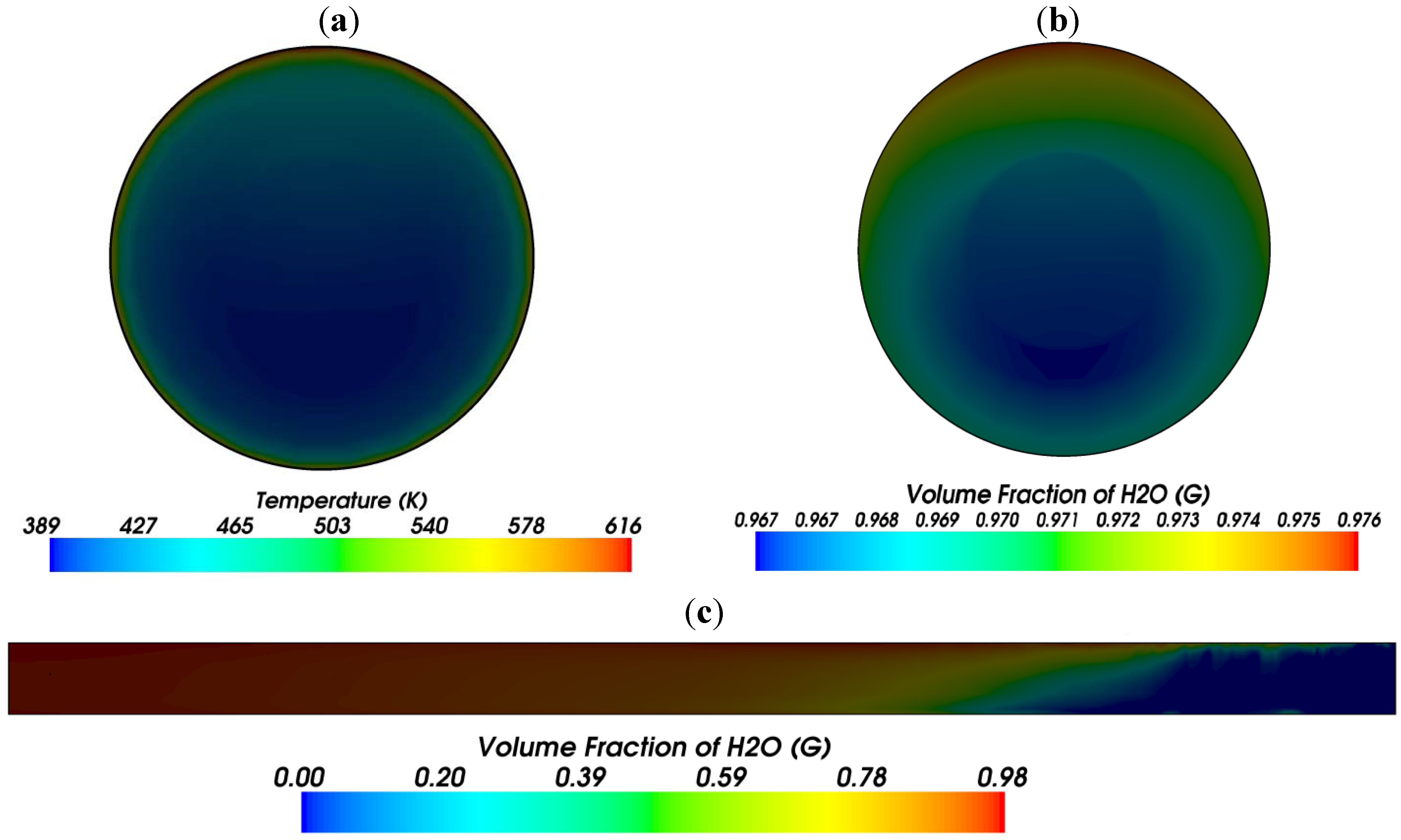
Figure 5 shows some simulation results for a 0.01 m diameter tube with flow rate of 15 kg/h (or 0.0042 kg/s) at noon time in a typical summer day.
Figure 5a shows temperature distribution of a water-steam mixture at the tube outlet, while
Figure 5b shows the volume fraction of steam generated relative to water at the outlet. Both graphs show that water temperature, hence steam volume fraction at the water-tube interface, is higher than that in the middle of the tube. This is because the water and steam layers are in contact with the hot metallic tube. In contrary, the lowest temperature, and hence the lowest steam volume fraction is shown in the middle of the water tube as it receives less energy. Both graphs also show that both temperature and steam volume fraction are higher on the upper half of the tube outlet than that of the lower half. This is due to the fact that water density reduces with increasing temperature, so higher temperature water and steam rise on top of the colder ones. This is also clear in
Figure 5c which shows the volume fraction of steam at a cross sectional plane across the tube length.
Figure 5c is intentionally drawn not to scale,
i.e., the ratio of tube length to its diameter has been distorted to show the buildup of steam during its passage across the tube.
In the next section, quantitative and qualitative analysis of steam emerging from the outlet will be carried out. A comparison between two systems having diameters of 0.005 m and 0.01 m, respectively, is performed. Changing tube diameter is responsible for changing the absorber area according to Equation (1), and hence the concentration ratio and flow speed inside the tube are changed. A set of six flow rates have been tested, namely 7, 8, 9, 10, 11 and 15 kg/h (corresponding to 0.0019, 0.0022, 0.0025, 0.0028, 0.0031 and 0.0042 kg/s, respectively) and the water-steam has been investigated qualitatively and quantitatively at the tube exit.
Figure 5.
Steam outlet (a) temperature distribution; (b) volume fraction and (c) volume fraction at a cross sectional plane across the tube axis (not to scale) for a 0.01 m diameter tube with flow rate of 15 kg/h (0.0042 kg/s) at noon in summer.
Figure 5.
Steam outlet (a) temperature distribution; (b) volume fraction and (c) volume fraction at a cross sectional plane across the tube axis (not to scale) for a 0.01 m diameter tube with flow rate of 15 kg/h (0.0042 kg/s) at noon in summer.
4. System Performance
As discussed above, the system is proposed to operate under ambient temperature and DNI in two selected days in summer and winter, respectively, as shown in
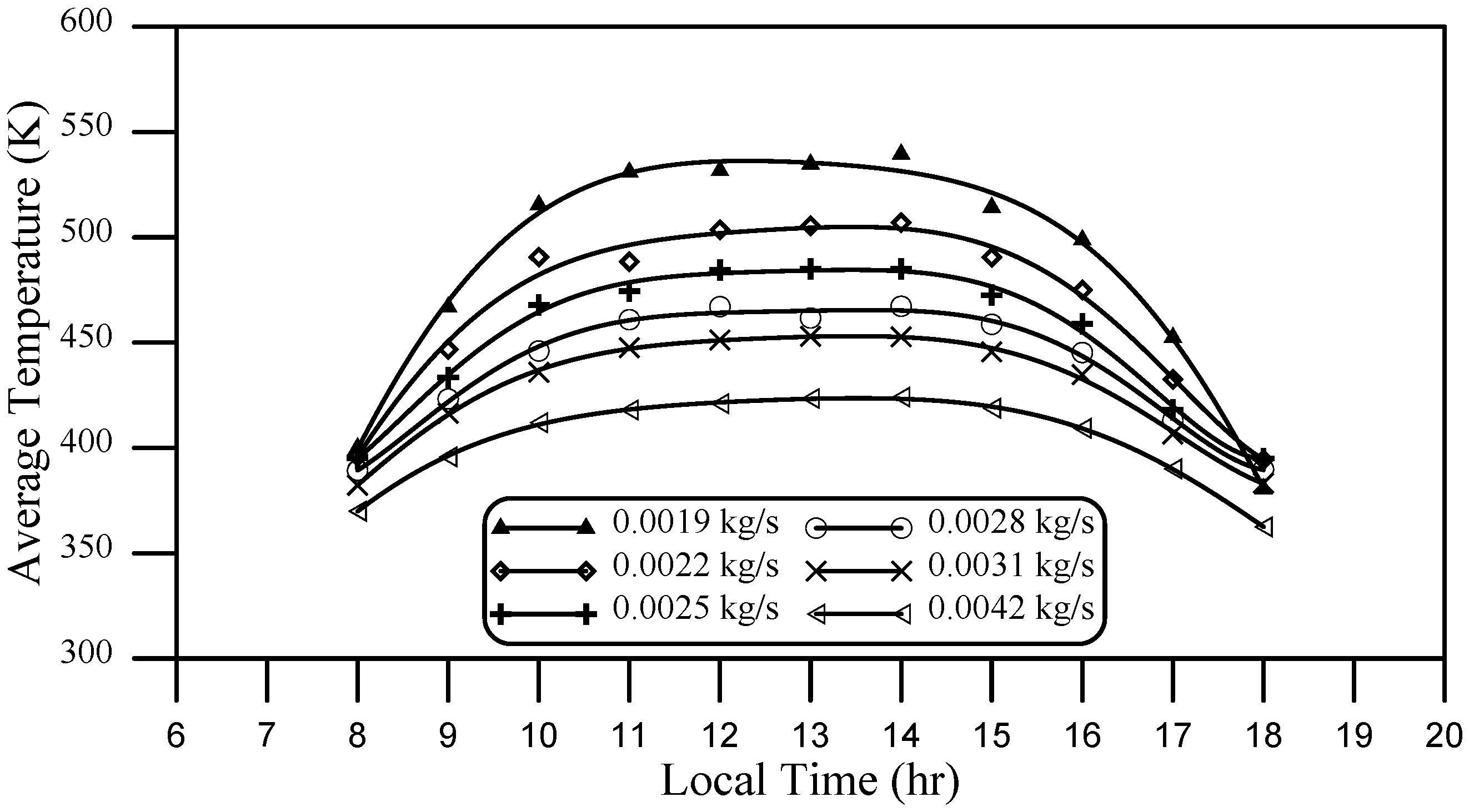
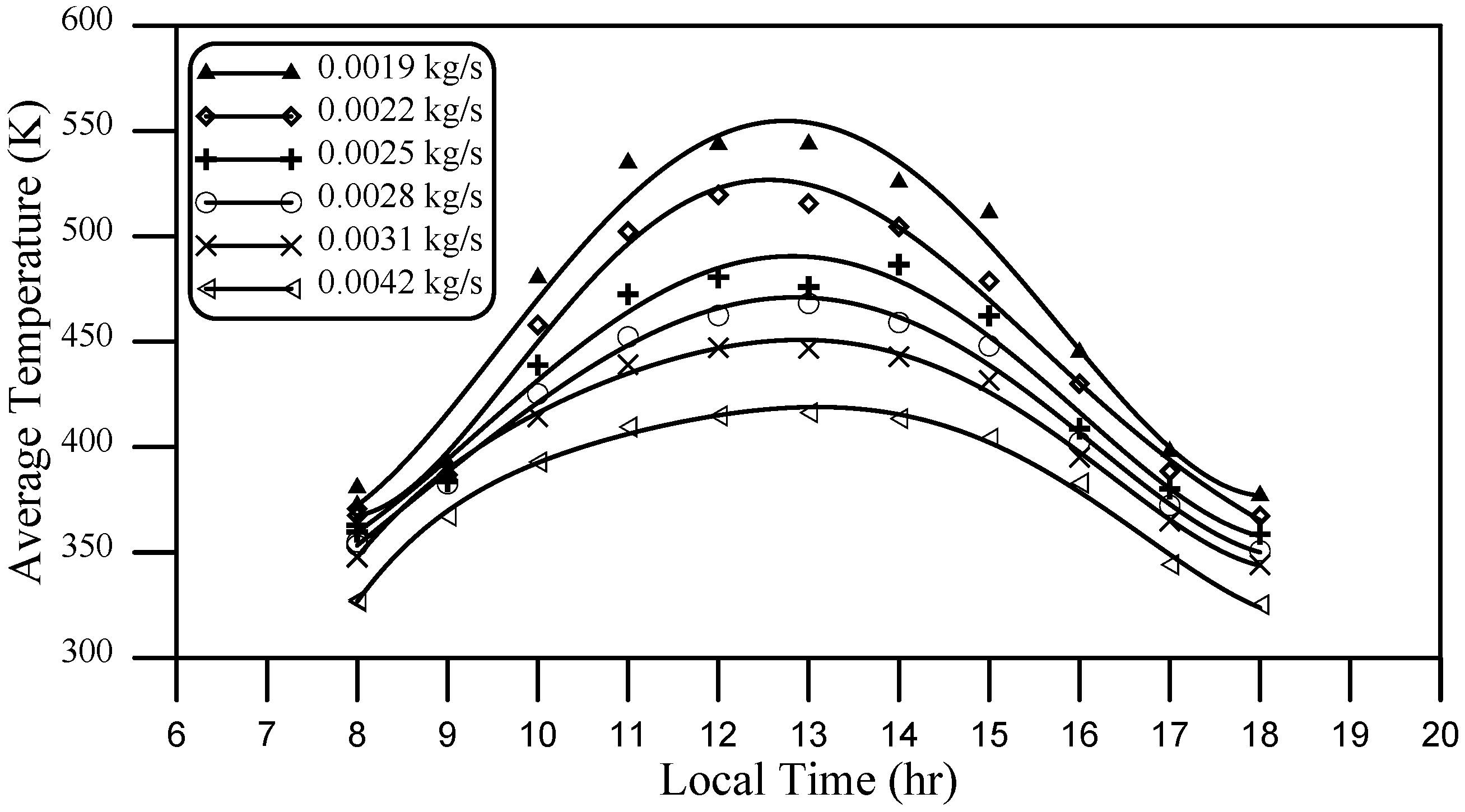
Figure 4. The simulation is performed for each hour by inputting the ambient temperature and DNI values to the model and assuming the water inlet has a temperature equal to the ambient temperature at that hour. Simulations have been performed for the flow rates mentioned above. Average temperature profiles of the water/steam mixture at the outlet of the 0.005 m diameter pipe in summer are calculated and shown in
Figure 6. As expected, increasing the flow rate resulted in a reduction of the average temperature of the outlet mixture. A similar behavior ocurrs for the daily profile of the 0.005 m diameter pipe in winter with a lower average outlet temperature as shown in
Figure 7 (in comparison with that of
Figure 6). In both graphs, the average steam temperature is directly proportional to both the solar radiation intensity and ambient temperature as shown in
Figure 4 and
Figure 11 and as will be discussed below.
Figure 6.
Daily profile of average output temperature for a 0.005 m diameter tube on a typical summer day.
Figure 6.
Daily profile of average output temperature for a 0.005 m diameter tube on a typical summer day.
Figure 7.
Daily profile of average output temperature for a 0.005 m diameter tube on a typical winter day.
Figure 7.
Daily profile of average output temperature for a 0.005 m diameter tube on a typical winter day.
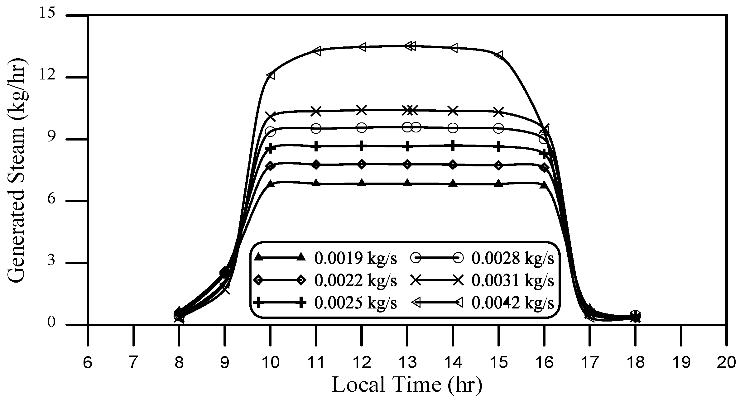
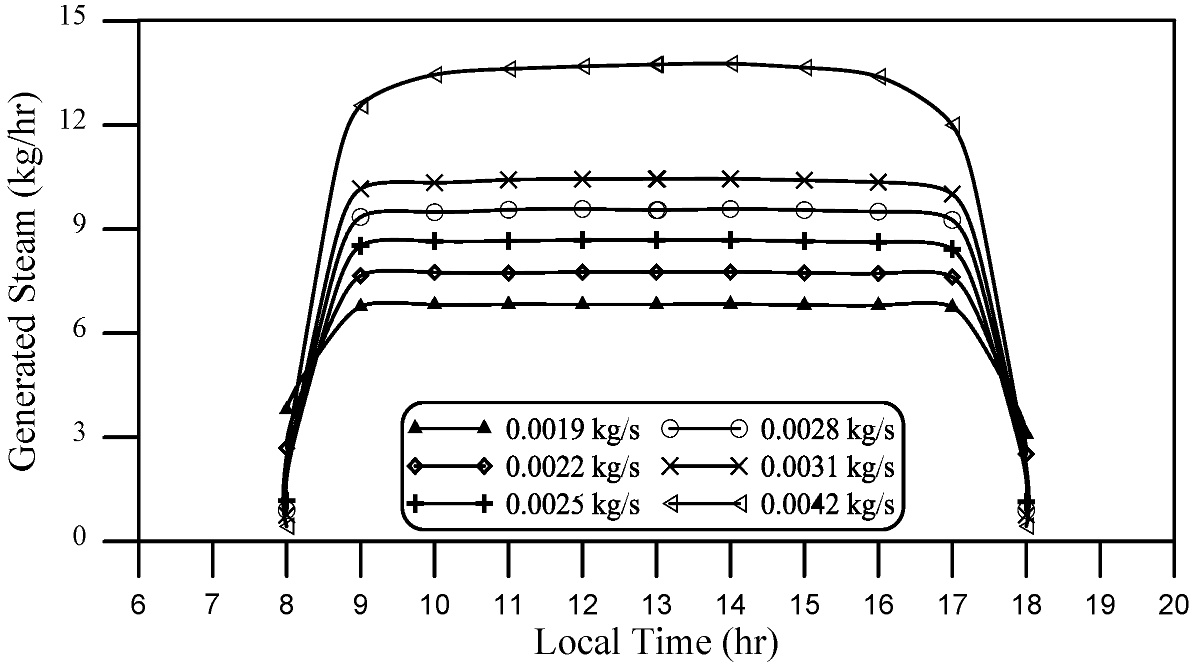
Rate of steam generated is then investigated by evaluating the mass of water that has been converted into steam again for the 0.005 m diameter pipe in summer and winter, which are shown in
Figure 8 and
Figure 9, respectively. These graphs show that a saturation of steam generation is established on either side of noontime with a rate of generation proportional to the inlet flow rate. Rate of generated steam in winter shown in
Figure 9 has a narrower profile width as compared to that of
Figure 8. This is due to the lower values of both DNI and water inlet temperature in winter than in summer (this is obviously due to the later sunrise and earlier sunset times in winter as compared to summer days; also ambient temperature in summer day is much higher than that of winter day).
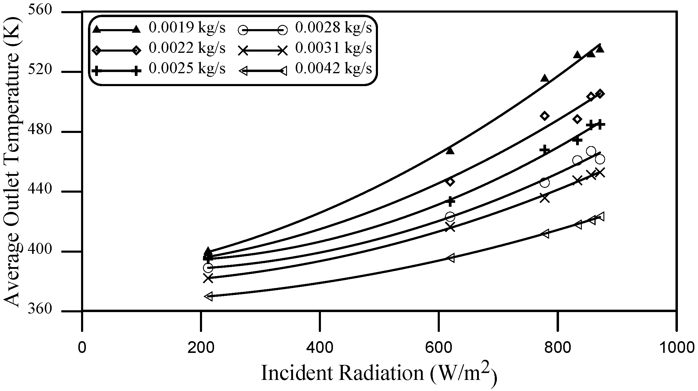
Average outlet temperature and generated steam mass rate are higher in summer than those of winter for the 0.01 m diameter pipe because both the solar radiation intensity and ambient temperature are higher in summer than that in winter. Average outlet temperature has been graphed against incident solar radiation in
Figure 10.
Figure 8.
Daily profile of rate of generated steam mass for a 0.005 m diameter tube in a summer day.
Figure 8.
Daily profile of rate of generated steam mass for a 0.005 m diameter tube in a summer day.
Figure 9.
Daily profile of rate of generated steam mass for a 0.005 m diameter tube in a winter day.
Figure 9.
Daily profile of rate of generated steam mass for a 0.005 m diameter tube in a winter day.
Figure 10.
Average outlet temperature with increasing incident solar radiation for the 0.005 m tube in summer.
Figure 10.
Average outlet temperature with increasing incident solar radiation for the 0.005 m tube in summer.
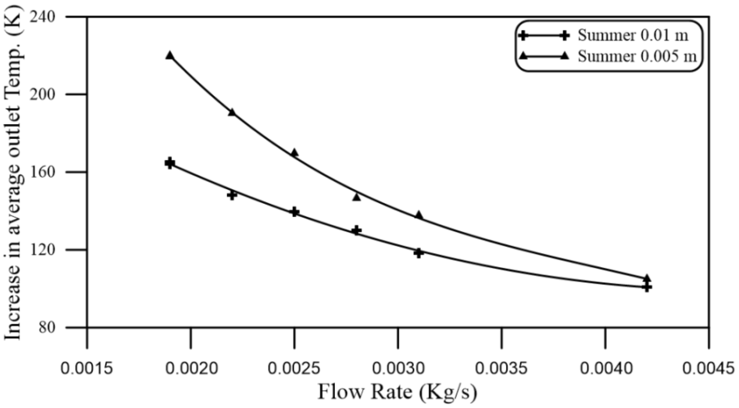
A nonlinear increase of temperature is due to the effect of increasing ambient temperature along with increasing solar radiation. The outlet temperatures increase above the inlet at noon for the two tube diameters under investigation in the proposed summer day as a function of water flow rate is shown in
Figure 11.
Figure 11.
Increase in the average outlet temperature for the 0.005 m and 0.01 m tubes on a summer day.
Figure 11.
Increase in the average outlet temperature for the 0.005 m and 0.01 m tubes on a summer day.
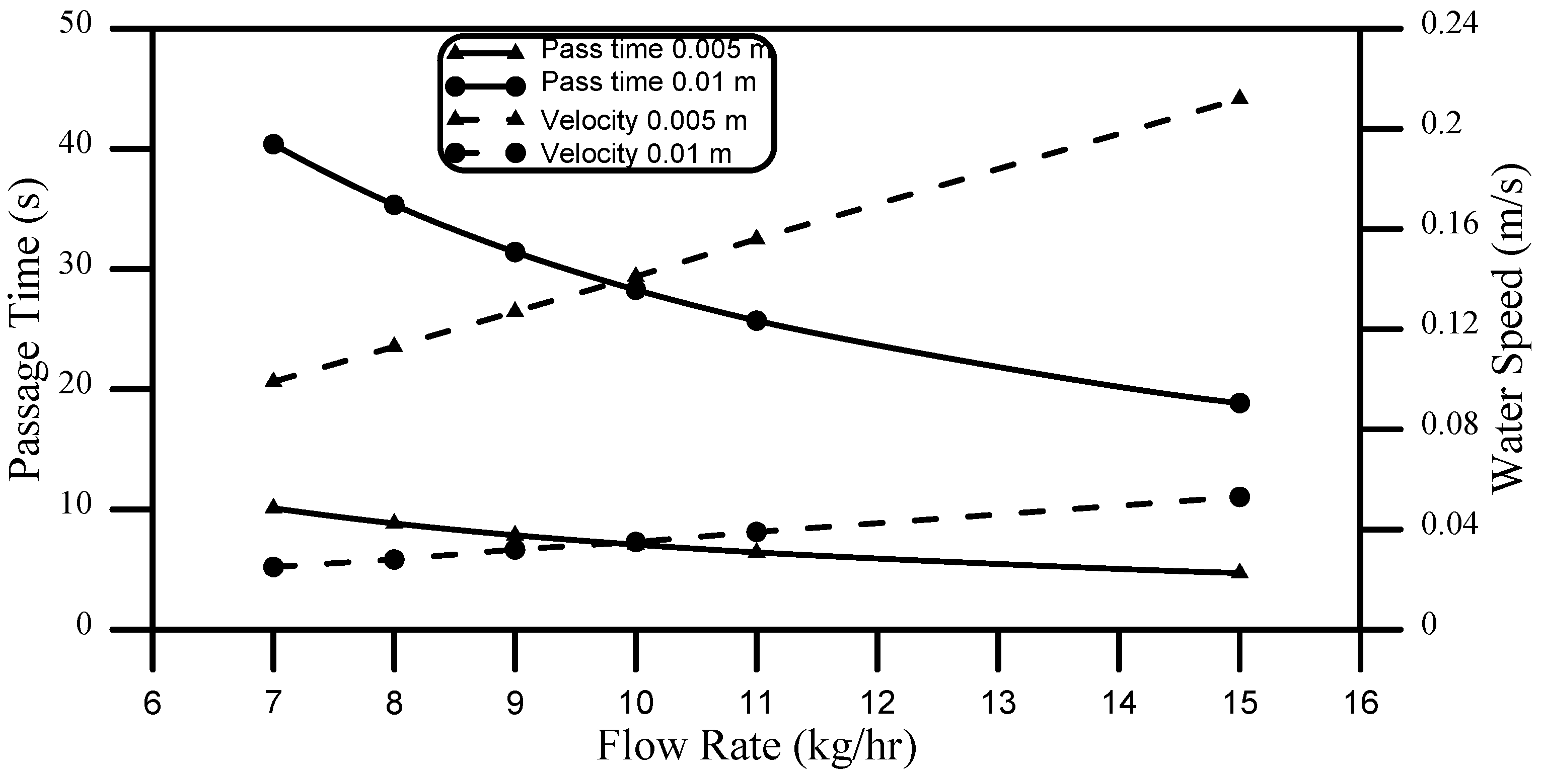
Increasing flow rate shows an asymptotic reduction of the average outlet temperature for both tubes as clearly shown in the figure. The narrower tube has an average outlet temperature increase of about 220 K at a flow rate of 0.0019 kg/s, corresponding to an increase of about 165 K at the same flow rate. Both tubes have nearly the same average outlet steam temperature increase of about 105 K at a flow rate of 0.0042 kg/s. This is because of the reduction in the passage time of water flowing inside the tube as a result of increasing water flow rate and hence water speed that is shown in
Figure 12. This graph represents calculations of both passage time and speed of water upon entering the inlet based on the values of tube diameter, length and the flow rate of water inside the tube. These calculations are valid only for water phase inside the tube. Once water in the liquid phase changes to steam phase, its volume increases greatly, hence, its speed and passage time will vary greatly depending on the location of steam inside the tube.
Figure 12.
Passage time and velocity of water inside the 0.005 m and 0.01 m diameter tubes.
Figure 12.
Passage time and velocity of water inside the 0.005 m and 0.01 m diameter tubes.
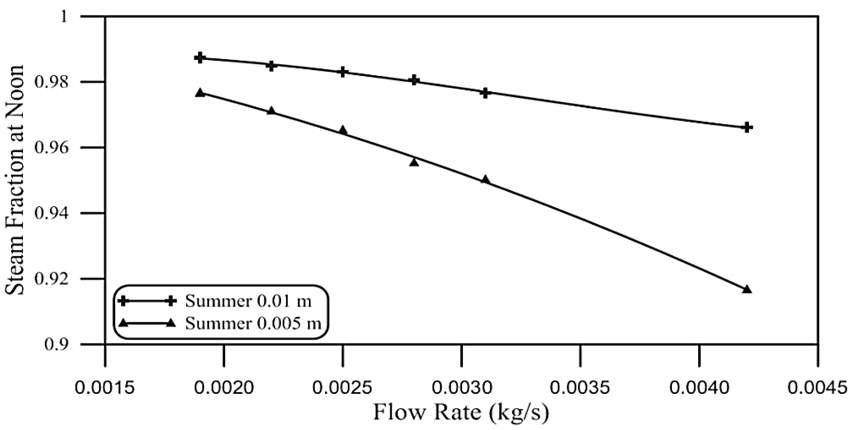
Generated steam fraction at noon time has been extracted from the simulation data, which expresses the mass of seam generated to water mass at the pipe outlet. This is graphed as a function of inlet flow rate for two tube diameters of 0.01 m and 0.005 m, respectively, in the proposed summer day as shown in
Figure 13. The wider the tube, the higher the steam fraction in spite of the average outlet temperature (cf.
Figure 11). This is because with a narrower diameter, the average temperature is affected by the temperature of the water near the outer tube surface which can be very high. On the other hand, the tube with the wider diameter has better distribution of heat at the outlet surface, hence, produces more steam.
Figure 13.
Steam fraction at noon for the 0.005 m and 0.01 m tubes on a summer day.
Figure 13.
Steam fraction at noon for the 0.005 m and 0.01 m tubes on a summer day.
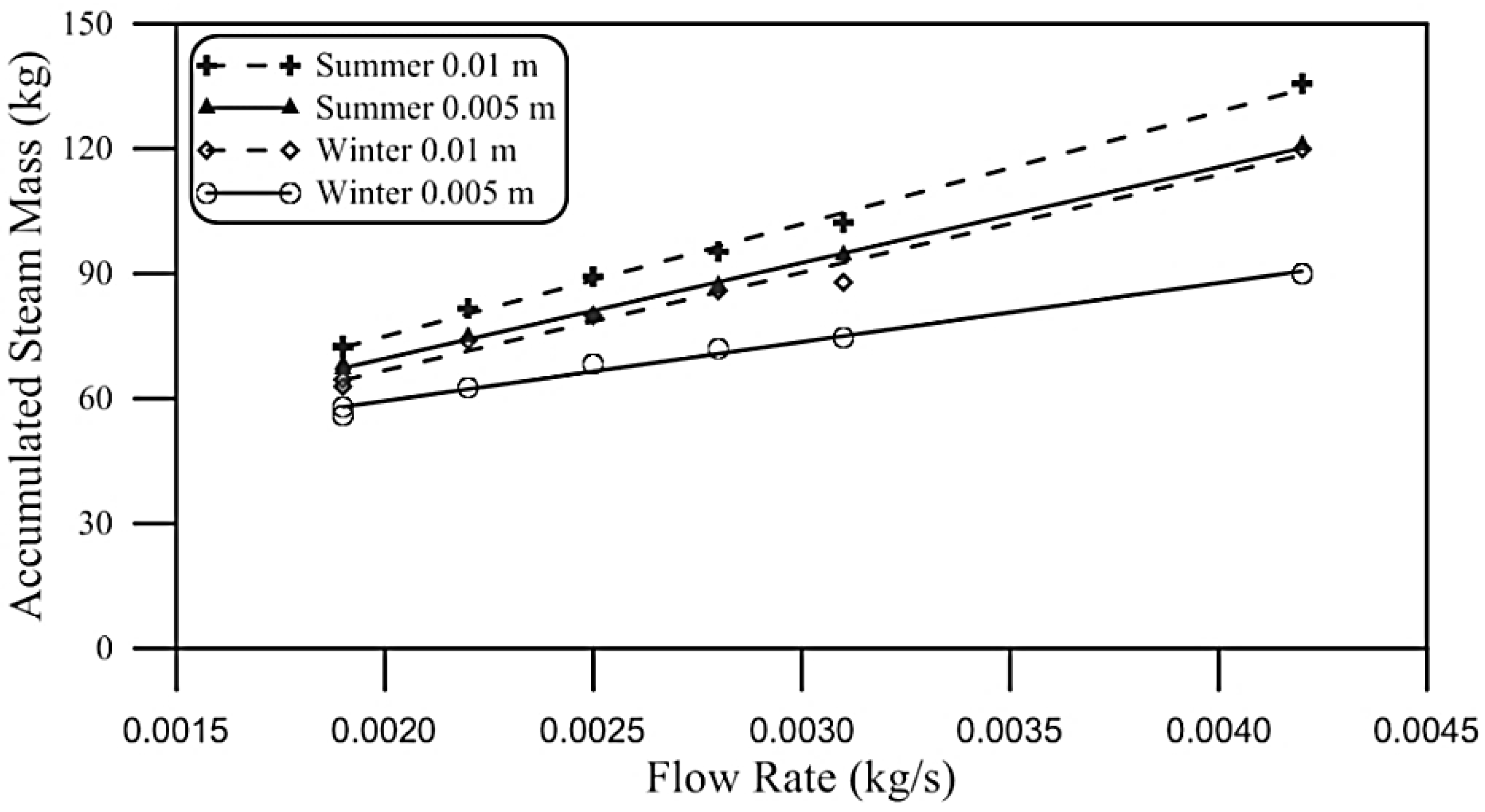
Figure 14 shows the daily accumulated steam mass in kg as a function of water flow rate for the two proposed diameters and their performance in winter and summer, respectively. Simulations show that for achieving a higher accumulated steam mass, the choice of the pipe diameter depends mainly on the intensity of solar radiation. In this figure, the 0.005 m diameter pipe generates a higher steam mass on a summer day than the 0.01 m diameter pipe on a winter day in spite of its narrower diameter. The 0.005 m diameter pipe’s performance is the lowest in winter days.
Figure 14.
Accumulated steam mass over the day for the 0.005 m and 0.01 m tubes in winter and summer, respectively.
Figure 14.
Accumulated steam mass over the day for the 0.005 m and 0.01 m tubes in winter and summer, respectively.
Qualitative analysis of the system performance depends on the structure of the output. In many cases, superheating is required to get a better steam temperature. This may be done by exposing the steam to additional solar energy for better steam quality. To study the quality of the steam generated, analysis of the outlet profiles of steam temperature has been performed to investigate the accumulated steam whose temperature is over 423 K as shown in
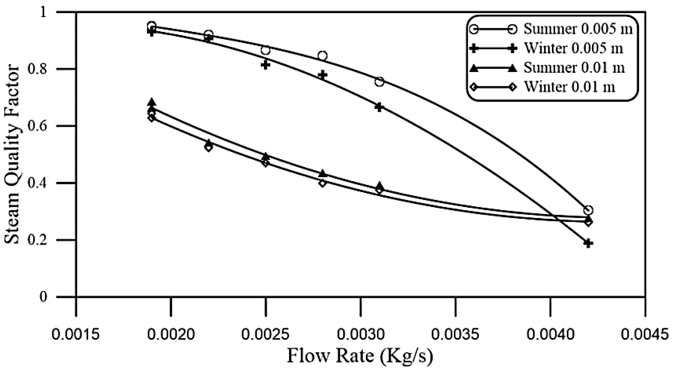
Figure 15 for the two proposed pipe diameters in winter and summer, respectively. The narrower tube showed better performance in terms of steam quality in both winter and summer, with an optimal flow rate of 0.0028 kg/s. On the contrary, the wider pipe showed a performance that is inversely proportional to the water flow rate. This is reflected in
Figure 16 which shows the steam quality factor for the two proposed pipe diameters in both winter and summer respectively as a function of water flow rate. Steam quality factor is calculated by Equation (7):
Figure 15.
Accumulated steam whose temperature is over 423 K for 0.005 m and 0.01 m tubes in winter and summer, respectively.
Figure 15.
Accumulated steam whose temperature is over 423 K for 0.005 m and 0.01 m tubes in winter and summer, respectively.
In some cases, high steam temperature is required for industrial purposes for example. Overheating may be used for achieving such high temperatures. For system optimization or for specific steam temperature demands, steam quality factor at that temperature may be calculated in order to investigate the performance at that specific temperature and determine the tube length for overheating process.
Figure 16.
Steam quality factor for the 0.005 m and 0.01 m tubes in winter and summer.
Figure 16.
Steam quality factor for the 0.005 m and 0.01 m tubes in winter and summer.
5. Conclusions
In this paper, analysis of steam generated from a water pipe exposed to concentrated solar radiation has been performed. Steam is generated from two proposed pipes with diameters of 0.005 m and 0.01 m, respectively, containing water flowing with different flow rates. As expected, increasing water flow rate reduced the average outlet temperature because of the reduction in the residence time of the water flowing inside the pipe. Quantitatively, an average increase of outlet temperature was about 220 K and 165 K for pipe diameters of 0.005 m and 0.01 m, respectively, at a flow rate of 0.0019 kg/s in summer. On the contrary, it was found that steam fraction was higher for the 0.01 m diameter pipe than that of the 0.005 m one for all flow rates. On the other hand, overheated steam was generated from the narrower pipes regardless of the solar radiation intensity, and it decreased with increasing water flow rate. A qualitative investigation shows that daily accumulated steam mass whose outlet temperature >423 K for the 0.005 m tube was maximum (about 74 kg/day and 53 kg/day in summer and winter respectively, both at a flow rate of 0.0028 kg/s) compared to that of the 0.01 m tube (about 50 kg/day and 40 kg/day in summer and winter, respectively, both at a flow rate of 0.0019 kg/s). Steam quality calculations show that the 0.005 m tube should be chosen if a high quality steam is desired. Otherwise, the 0.01 m diameter tube should be selected if a higher quantity of steam is required regardless of its quality.


