1. Introduction
In the last decades a great effort has been performed in order to analyze the technologies related to the exploitation of low-medium temperature heat sources. In this framework, the Organic Rankine Cycle (ORC), a Rankine cycle that uses an organic fluid, is one of the most interesting and promising of such technologies. The components of an ORC layout are the same as those of a conventional Rankine cycle. In fact, both systems include pumps, expanders and heat exchangers. As concerns the working fluid, water is used in a conventional Rankine cycle, while the ORC system uses an organic fluid, due to its many advantages in case of low-temperature heat sources. In particular, their high molecular weight allows one to reduce the volumetric flow rates and the expansion ratio. Thus, single-stage turbines can be used, also increasing the condensing pressure above the atmospheric one. Then, the slope of saturated vapor curve in the (
T,
s) chart is positive (“dry” fluid) for the majority of the organic fluids, possibly avoiding the superheating process [
1,
2,
3,
4], determining a consequent reduction of system capital costs. Furthermore, the critical temperatures of the organic fluids are typically lower than the one of water. Such circumstance, as shown in many studies [
4,
5,
6], allows one to achieve reasonable efficiencies even in case of low-temperature heat sources.
Therefore, Organic Rankine Cycles are particularly attractive in case of low-medium temperature heat sources. Consequently, a number of papers are available in literature investigated different aspects of ORC systems. A comprehensive overview of ORC technology is provided by Bertrand
et al. [
7], investigating existing and potential ORC power plants. Similarly, an interesting analysis of the different ORC applications is presented by Quoilin
et al. [
5], who present a market review including cost figures, a detailed technical analysis and an overview of the present trends in research and development for the next generation of ORC. The research group of Quoilin
et al. has presented several studies about ORC systems, such as the design of a small-scale solar ORC for rural electrification purposes [
8]; the development of a simulation model in Engineering Equation Solver (EES) [
9] in order to select the capacities of the components included in the system; numerical and experimental analyses of an ORC system which uses R-123 as working fluid [
10]. Several of those studies demonstrated the viability of utilizing a mass-produced compressor as an expander in a small scale ORC.
The majority of the papers available in literature, regarding ORC systems, investigate the appropriate selection of the fluid, which is strongly related to the heat source used [
1,
2,
6,
11,
12,
13,
14,
15,
16,
17]. For example, several organic fluids have been investigated by Calise
et al. [
6] to evaluate ORC performance varying heat source temperature from 120 to 300 °C. Results showed that
n-pentane,
n-butane and isobutane are appropriate fluids for a wide range of heat source temperature levels, from low to high. R245fa, instead, is recommended up to 170 °C.
ORC are often coupled with renewable energy sources, due to their capability to operate at acceptable efficiency even when the driving temperature is low. In fact, several papers are available in literature presenting different combinations of solar [
18] and/or geothermal [
19,
20] systems coupled with ORC power plants. As an example, Franco and Villani [
21] analyzed the exploitation of water-dominated geothermal fields at low temperature, showing brine specific consumptions, ranging from 20 to 120 kg s
−1 for each net MW produced. Second Law efficiency of the plants ranges from 20% to 45% depending on the brine inlet temperature and on the selection of the energy conversion cycle. Astolfi
et al. [
19,
20] investigated binary ORC power plants for the exploitation of low-medium temperature geothermal sources in the temperature range of 120–180 °C and defining the optimal combination of fluid, cycle configuration and cycle parameters. Results showed that supercritical cycles, employing fluids with a critical temperature slightly lower than the temperature of the geothermal source, lead to the lowest electricity cost. El-Emam and Dincer [
22] presented thermodynamic and economic analyses for a geothermal regenerative ORC. The authors assessed that the ORC evaporator and condenser showed the highest exergy destruction rates. Habka and Ajib [
23] investigated some hybrid integrations of cogeneration plants based on ORC driven by low-temperature geothermal water. The results showed excellent performance in terms of power production and exergy efficiency.
Several studies investigating the integration of ORC and high temperature solar systems are also available. As an example, Calise
et al. [
24] investigated an ORC system coupled with parabolic solar thermal collectors. Authors evaluated the off-design performance of the plant and the results showed that the heat source mass flow rate is a key parameter in net power generation. Wang
et al. [
25] presented a solar-driven regenerative ORC system. Here, the parameter optimization using the daily average efficiency as objective function. Authors found that a continuous and stable operation of the system may be achieved only when a thermal storage tank is used.
The two above mentioned configurations (solar-ORC and geothermal-ORC) are often analyzed from the exergetic point of view. Al-Sulaiman [
26] presented an in-depth exergetic analysis of ORC power systems driven by parabolic trough solar collectors, showing that the exergy efficiency may vary from 20% (R600a) up to 26% (R134a). The main source of exergy destruction is due to the solar collectors and the overall exergetic improvement potential of the systems considered is around 75%. Maraver
et al. [
27] presented an optimization model of the ORC in order to define the best system performance in terms of its exergy efficiency, using different working fluids and system layouts.
As shown before, a number of studies are available in literature presenting different analyses (thermodynamic, exergetic, optimizations,
etc.) of solar-ORC and geothermal-ORC systems [
28]. However, the possibility to combine solar source, geothermal source and ORC power systems in a single plant is scarcely investigated. Only a few works are available in literature investigating such configuration. In particular, Astolfi
et al. [
29] analysed a combined concentrating solar power system and a geothermal binary plant powering an ORC, and they obtained a levelized costs of electricity of 145–280 €/MWh (competitive value with respect to large, stand-alone concentrating solar power plants [
29]) depending on the location of the plant. Tempesti
et al. [
30,
31] investigated the combination of geothermal heat sources and solar powering a ORC system, and also Zhou
et al. [
32] studied these hybrid plants, concluding that the cost of electricity production can be reduced by 20% when this technology is used instead of the stand-alone Enhanced Geothermal System (EGS) [
32]. Zhou [
33] developed a model simulation of a hybrid geothermal solar both subcritical and supercritical ORC using Aspen to compare the two configurations, and results showed that the solar to electricity cost of supercritical ORC is about 1.5%–3.3% less than those of the subcritical system. Ghasemi
et al. [
34] developed a model for an existing organic Rankine cycle (ORC) utilizing a low-temperature geothermal brine, validated by experimental data. The existing system is retrofitted with a low-temperature solar trough system. This hybridization strategy achieves a significant boost in the net output power of the system compared to the geothermal ORC. This hybridization approach also allows one to enhance the extraction of geothermal energy. The hybrid system shows higher second-law efficiency (up to 3.4% difference) compared to combined individual geothermal and solar systems. Authors concluded that the hybrid system is a better option than individual geothermal and solar systems at all ambient temperatures, from the energetic point of view. The economic problem was not addressed in this study. A low-temperature hybrid solar-geothermal ORC system was investigated by Ruzzenenti
et al. [
35]. Authors evaluated the environmental sustainability of a small combined heat and power (CHP) plant operating through a 50 kW Organic Rankine Cycle (ORC) coupled with low temperature (90–95 °C) geothermal energy and solar energy (collected by evacuated, non-concentrating solar collectors). The environmental impact assessment was performed through a Life Cycle Analysis and an Exergy Life Cycle Analysis. Authors found that the reservoir is suitable for a long-term exploitation of the designed system, however, its sustainability and the energy return is edged by the surface of the heat exchanger and the limited running hours due to the solar plant. Therefore, in order to be comparable to other renewable resources or geothermal systems, the system needs to use existing wells, previously abandoned. A more complex hybrid solar-geothermal ORC trigeneration system was recently presented by Buonomano
et al. [
36]. The hybrid system is based on: 6 kWe micro Organic Rankine Cycle (ORC); a 30 kWf single stage H
2O/LiBr absorption chiller; a geothermal well (at 95 °C); a solar field obtained by new prototypal flat-plate evacuated solar collectors. Geothermal energy is obtained by a combination of a downhole heat exchanger and by fluid extraction. Solar energy is used only to boost ORC power production. The system can produce simultaneously electrical energy, cooling energy and thermal energy for a hotel located in Ischia (South of Italy). The system showed excellent energy performance indexes. From the economic point of view, good results are also obtained. In fact, in the worst operating conditions the Simple Payback Period is 7.6 years, decreasing to 2.5 years in the most convenient considered scenario (public funding and full utilisation of the produced thermal energy).
The literature review presented in this section shows that although solar-ORC and geothermal-ORC are investigated in detail, only a few pioneering theoretical studies analyze the possibility to integrate solar and geothermal sources with ORC power plants. Although these papers present the significance to introduce this innovative hybrid layout, a number of topics are still not sufficiently addressed. As a consequence, much additional work is needed to investigate in detail all the possible aspects of this innovative layout. In particular, the majority of the cited papers are based on steady thermodynamic calculations of the performance of the hybrid solar geothermal systems, omitting 1-year dynamic simulations of the system. Similarly, these papers do not include in-depth exergy and economic analyses of the system. On the basis of this framework, this paper aims to implement this topic, introducing several major innovations with respect to the methodologies and the findings available in literature, namely:
1-year dynamic simulation: this paper presents the development of a dynamic simulation model of an Organic Rankine Cycle (ORC) fed by solar and medium-enthalpy geothermal energy. Zero-dimensional energy and mass balances simulate the ORC model with Engineering Equation Solver (EES), which allows one to evaluate the off-design performance of the plant setting the geometrical features of ORC heat exchangers and the design conditions of the turbine. Moreover, the simulation model has been implemented in a more complex TRNSYS project in order to consider both geothermal and solar sources, simulating solar collectors, geothermal well, heat exchangers, pumps, tank and controllers. Therefore, a dynamic simulation of the hybrid plant has been obtained. In the authors’ knowledge, none of the papers available in literature includes a 1-year dynamic simulation of a hybrid solar geothermal ORC system, which allows one to vary the ORC driving temperature as a function of the available solar radiation.
Exergy analysis: a detailed exergetic analysis is performed, aiming at detecting the sources and the magnitude of irreversibilities within the components of the plant and within the plant as a whole. Such analysis allows one to calculate the magnitude of the irreversibilities and to analyze possible actions to reduce such losses in the system. An exergetic optimization has been also performed with the scope to calculate the set of design parameters, minimizing the overall system exergy destruction.
Thermo–economic optimization: a rigorous optimization has been implemented varying the main design parameters (such as collectors area and tank volume). Detailed heuristic/deterministic algorithms have been implemented in order to calculate the set of the design parameters minimizing the payback period of the system.
The analysis presented in this paper will be a useful tool for system designers. In fact, the 1-year dynamic simulation model allows one to predict system performance for whatever period of the year. Such a tool also allows one to customize system design parameters as a function of weather data, geothermal features and user energy demand profile. In addition, both energetic and thermo-economic optimizations are useful tools for the designer, which allow one to reduce the manufacturing and developing costs of this emerging technology. Therefore, the model presented in this paper can be usefully utilized in order to design and manufacture optimized solar-geothermal-ORC systems. An optimized design of these systems is crucial in order to promote their commercialization and to improve the profitability for the final user.
2. System Layout
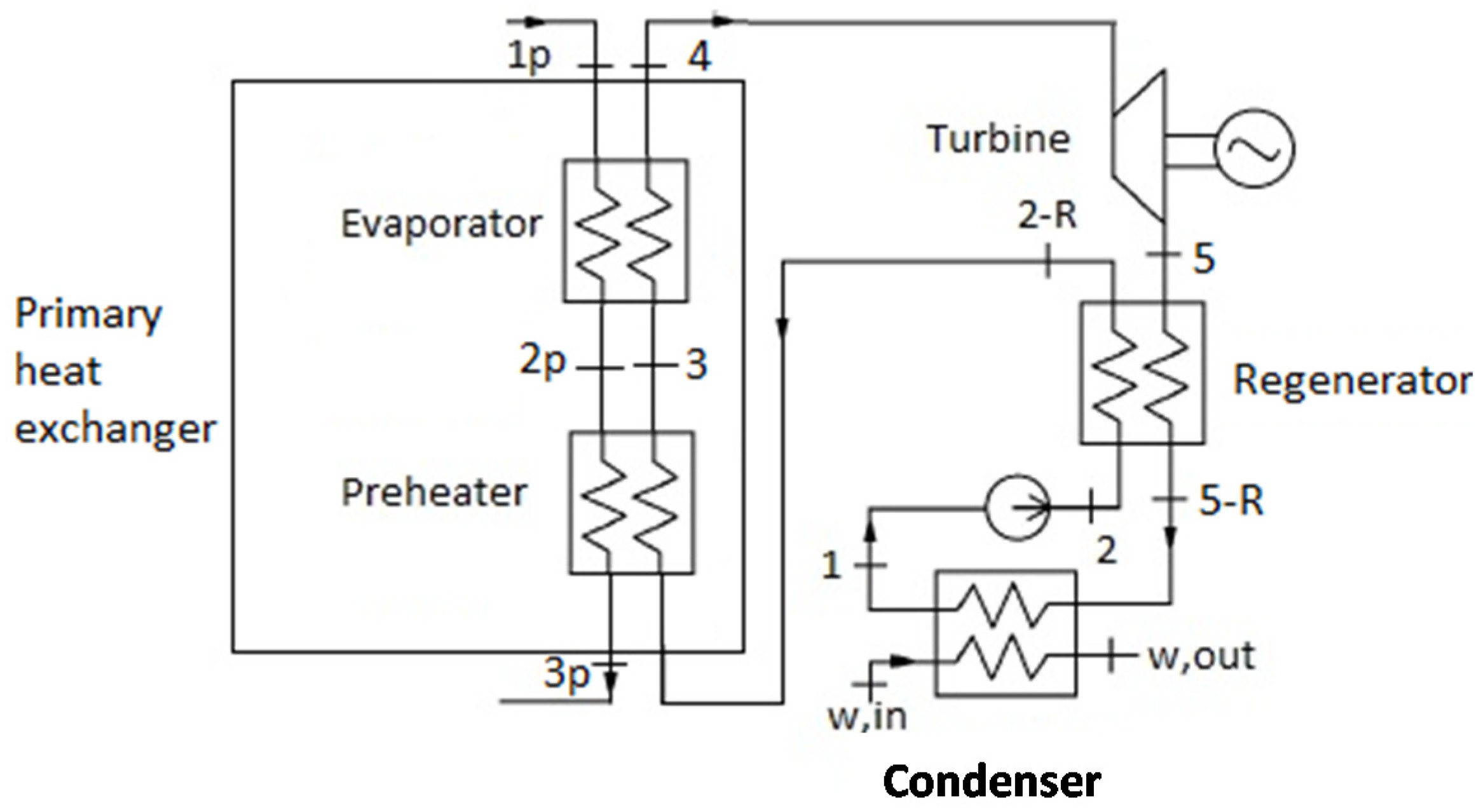
In this paper, the organic fluid receives thermal energy in the primary heat exchanger, which is considered as a single component. According to the literature cited before [
1,
2,
3,
4], a superheater is not considered. Furthermore, the presented ORC layout also includes a regenerator, in order to recover thermal energy from the turbine outlet stream by preheating evaporator inlet fluid. Several authors [
3,
4,
37,
38,
39,
40] showed that the use of this component improves the energy efficiency of the cycle. In addition, the ORC is used in cogeneration mode. In fact, the condenser heats water from 40 to 50 °C and the water mass flow rate is varied as a function of the available ORC thermal capacity.
The layout of the ORC subsystem considered (
Figure 1) is based on the Heat Transfer Fluid (HTF) configuration, as shown in previous works [
6,
24]. This configuration involves the use of a secondary fluid to transfer the thermal power from heat sources to the ORC working fluid. The HTF system involves some advantages with respect to the Direct Vapor Generating (DVG) configuration,
i.e., better control and the possibility to regulate cycle performance, although it is more expensive and complex and less energy efficient than DVG. As the present work is a based on the combined utilization of geothermal and solar energy, the DVG configuration cannot be applied. Therefore, diathermic oil is used to collect thermal energy from solar collectors and geothermal well to be subsequently supplied to the organic fluid in the primary heat exchanger of the ORC. In fact, 50 kg/s geothermal brine at the temperature of 160 °C supplies heat to the diathermic oil in a heat exchanger (Geothermal HE), providing a constant thermal energy flow. In addition, a 10,000 m
2 Parabolic Trough Collector (PTC) solar field raises the temperature of the diathermic oil. Considering the possible temperature achieved,
n-pentane is selected as organic fluid, in accordance with the results shown in reference [
6]. In fact, according to the results found in reference [
6] and to the findings of the majority of the papers cited in the previous section,
n-pentane shows one of the most suitable (
T,
s) diagrams, for the selected inlet hot fluid temperatures. A possible further improvement of system energetic and exergetic efficiencies could be achieved using mixtures from alkanes (e.g., butane/pentane mixtures). In fact, for such mixtures evaporation and condensation temperatures show temperature glides which better fit with hot fluid and cooling water temperature profiles. This will reduce exergy losses. Unfortunately butane/pentane mixtures are not available in conventional thermodynamic databases. Therefore, the implementation of such fluid will require a different work aiming at evaluating all its correlations.
Figure 1.
Organic Rankine Cycle (ORC) power plant.
Figure 1.
Organic Rankine Cycle (ORC) power plant.
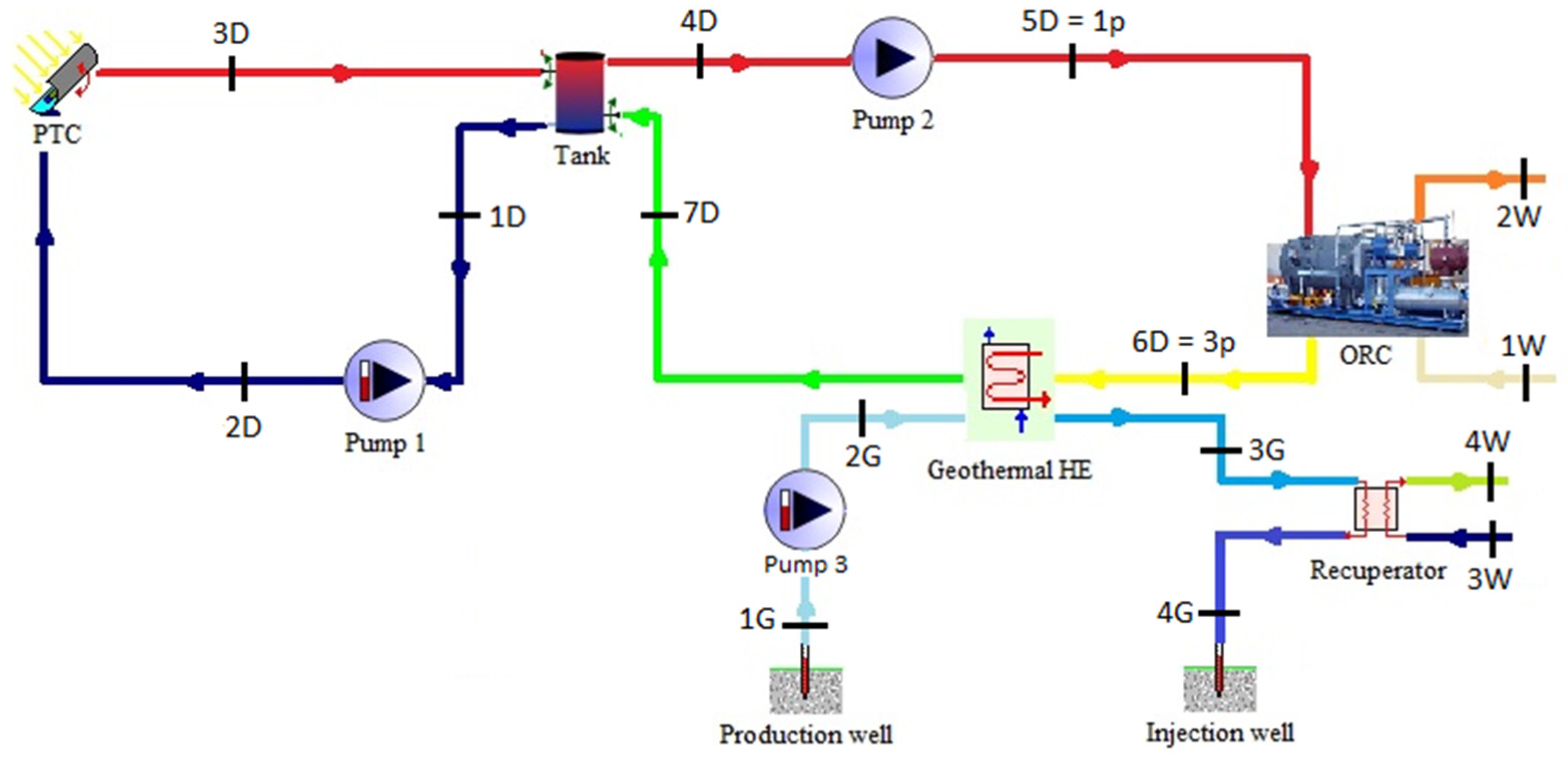
The overall system layout of the hybrid solar-geothermal power plant is shown in
Figure 2. The system includes PTC, geothermal wells, ORC (which is here shown as a single component), geothermal Heat Exchanger (HE), a storage tank, pumps and a recuperative heat exchanger.
The purpose of the storage tank is to decouple geothermal and solar loops in order to mitigate the typical fluctuations of the solar irradiation. In case of scarce or null availability of solar energy, the ORC plant is powered only by the geothermal source. Conversely, during daylight, Pump 1 is activated in order to provide solar heat to the stratified tank. Pump 2 brings the fluid from the top of the tank to the hot side of the ORC primary heat exchanger. Pump 1 is regulated by an on/off controller. In fact, it continuously measures and compares the temperatures of the diathermic oil at the bottom of the tank and the one of the solar collector’s outlet streams. When, the temperature of the fluid in the bottom of the tank is lower than the one at outlet of the PTC, Pump 1 remains activated. Note that Pump 1 is not a variable speed pump, as usually occurs in solar systems, in order to control solar field outlet temperature. In fact, one of the aims of this work is the investigation of the ORC performance as a function of the variations of its driving temperature. In addition, the utilization of a variable speed pump would lead to an ORC cycle operating at constant inlet temperature, previously investigated in references [
6,
18,
24,
36]. Pump 3 is regulated by an on/off controller, deactivating the pump when the temperature of the oil exiting the hot side of the ORC primary heat exchanger is higher than the one of geothermal brine. These strategies prevent any heat dissipation.
Figure 2.
Layout of solar and geothermal cycle.
Figure 2.
Layout of solar and geothermal cycle.
Finally, the goal of the recuperator is to recover additional thermal energy from the geothermal fluid. In fact, this component is used in order to recover the heat of the geothermal fluid exiting from the geothermal HE, producing hot water. In particular, the hot water flow rate is varied in order to achieve a constant temperature of the geothermal fluid to be re-injected in the well. Such temperature is set at 70 °C, in order to limit the depletion of the geothermal reservoir. At design condition, hot water is heated from 55 to 67 °C.
3. TRNSYS Simulation Model
In order to obtain a dynamic quasi-steady simulation of the system, ORC model developed in EES has been imported in TRNSYS environment [
41]. In particular, the EES model of the ORC system is included in TRNSYS environment using a built-in component (Calling EES) which is able to call EES sub-module of the ORC for each time-step of the overall TRNSYS simulation. This capability allows one to link TRNSYS and EES software. Obviously, specific additional connections have been performed in order to link ORC inlet and outlet temperatures and flow rates to the other components of the system included in TRNSYS project. TRNSYS software is used to model transient systems both in commercial and academic fields. This software includes a wide library of various built-in components often validated by experimental data. Some of the models of the components of system shown in
Figure 2 (
i.e., PTC, geothermal source, storage tank, geothermal HE and pumps) are taken from TRNSYS library. All these models are validated
vs. experimental data. Conversely, some new models (ORC, recuperator, exergetic calculators, economic analyses,
etc.) have been developed by the authors and linked to the TRNSYS environment. The simulation also requires additional components (not shown in
Figure 2) such as: a weather database, controllers, integrators and various calculators required in order to evaluate overall heat transfer coefficients of the geothermal HE and to perform exergetic and economic analyses. Finally, the model also includes a number of tools required to post process the data returned by the simulations.
For sake of brevity, the following section presents a brief description of the new models (exergetic and economic) proposed in this paper. Energetic models of the tanks, solar collectors, pumps and heat exchangers are well established and available in reference [
41]. The model of the ORC is shown in
Appendix A, whereas readers may refer to the previous papers for further details regarding the recuperator [
42].
3.1. Exergetic Model
As in the case of the ORC, no chemical process occurs in whatever system component. Therefore, also in TRNSYS environment, exergy balances may consider the sole physical exergy, neglecting the chemical one. Since all the fluids (diathermic oil and geothermal brine) are in liquid state, physical exergy can be calculated as follows:
is the constant volume fluid specific heat, which is assumed constant due to the small variations in temperature.
It should be noted the term
is often negligible compared to the other ones of the Equation (1), as is demonstrated by Calise
et al. [
43]. Hence, the equation can be simplified as shown in Equation (2):
This equation has been used to calculate physical exergy per unit mass for all the streams shown in
Figure 2.
Then, the exergy balance can be written for whatever component of the system and for the plant as a whole. It is worth noting that the exergy balance consists of an input term (exergetic fuel), representing the exergetic consumption and two output terms, namely: the exergetic product, being the useful exergetic effect and the exergy destruction which is representative of irreversibilities [
44].
Exergy destruction, efficiency defects and exergy efficiencies can be obtained by simple exergy balances for all the components included in the system. It is worth noting that the exergetic flow due to electrical power produced or consumed is numerically equal to the electricity produced or consumed [
44]. A special calculation has been performed in order to evaluate the exergy flow due to the solar radiation. Petela theorem has been considered by Equation (3):
where
A is equal to the collectors area,
I to the solar irradiation, and
Tsun to 3/4 of the black body temperature,
i.e., 4,350 K [
43].
In summary, exergy destruction and exergetic efficiency can be calculated as follows:
The previous equations represent the most common formulation of exergy efficiency for solar thermal collectors. Equations (3)–(5) typically lead to low exergetic efficiency values due to the significant difference between
Tsun and the average temperature of the fluid flowing in the collectors. To overcome this issue, some researchers have proposed a new approach which consists in referring the exergetic efficiency to the absorber plate temperature, rather than
Tsun.. Using this approach, an different definition of the exergetic efficiency of the solar collectors can be obtained (
) [
45]:
ORC
Exergetic analysis has been conducted for each component of the ORC subsystem. None of the ORC components involves chemical reactions. Therefore, only physical exergy related to the material and energy flows for each component have been considered for the formulation of exergy balances. Physical exergies for all the state points of the system are calculated as shown in ref. [
43].
The overall ORC plant exergetic performance has been calculated as follows:
where
is the efficiency defect of the
i-th component all ORC [
44].
Balance of the Plant (BOP)
In order to investigate the variations of the system performance during the year, power and exergy flows have been integrated and calculated on a specified time basis as follows:
where
and
are, respectively, the power and the exergy flow in MW, while
and
are, respectively, the accumulated energy and exergy, in MWh. Therefore, ORC energetic efficiency has been evaluated considering by Equation (22):
System exergetic efficiency is calculated by Equation (23):
Finally, solar fraction has been calculated as follows:
3.2. Economic Model
A detailed economic model has been implemented in order to calculate the overall thermo-economic performance of the system under investigation. In particular, capital costs of system components are related to the main design parameter and/or to the rated capacities of the components. Specific costs can be calculated on the basis of literature or manufacturers data:
BOP (including pipes, tanks, valves,
etc.) [
24]
Management and maintenance
In particular, management and maintenance costs are calculated as 2% of the components costs.
Specific revenues have been reported in
Table 1.
Table 1.
Specific revenues of the plant.
Table 1.
Specific revenues of the plant.
| Parameter | Value |
|---|
| Generated electricity from solar energy revenue | 0.34 €/kWh |
| Generated electricity from geothermal source revenue | 0.165 €/kWh |
| Thermal energy produced revenue | 0.052 €/kWh |
Such an approach allows one to dynamically calculate the capital cost of the system when one or more design parameters are changed. This is extremely useful in order to perform parametric analyses and optimizations as shown later on. Equation (27) is suggested by Taal
et al. [
48] and it is used in the case of shell and tube heat exchangers with titanium both on the shell side and tube side. This type of heat exchanger is used since the geothermal fluid is strongly corrosive and it passes through the shell side. The other cost equations are obtained from manufacturers’ data. All the capital costs include engineering costs, whereas possible insurance costs are neglected since their magnitude is marginal with respect to the remaining cost figures. Similarly, land costs are also neglected since the prototype is supposed to be installed in an isolated area where land cost is very small. The specific revenues related to the generated electricity are calculated considering the current legislation in Italy. In particular, data regarding costs and incentives are obtained by Gestore Servizi Energetici, GSE SpA [
49], Italian company, controlled by the Ministry of Economy and Finance, which provides incentives (feed-in tariffs) for the production of electricity from renewable sources. The incentives related to solar energy and geothermal energy are different. Therefore, the solar fraction has been calculated, as reported in Equation (24), in order to get the different contribution of the two renewable sources for the electrical energy production. In particular, the overall electrical production has been divided in two parts, proportionally related to the calculated solar fraction. Therefore, two different electrical productions are calculated, namely solar and geothermal, which can benefit of the two different feed-in tariffs. The revenue due to the thermal energy produced has been obtained by considering the current cost of the thermal energy. Note that the system also includes Management and Maintenance costs which must be considered among operating costs. Therefore, the SPB has been calculated as follows:
where
CC is the capital cost,
CF the cash flows and
OC the operating costs.
4. Results and Discussion
On the basis of the model presented in the previous sections, a case study has been analyzed. The plant is located in Naples, in the South of Italy, where the availability of the above presented geothermal resources is high. In this area, according to the Meteonorm weather database used in the simulations, the maximum radiation is equal to 1.01 kW/m
2. The daily radiation varies from 0.52 kWh/(m
2·day) on a cloudy winter day up to 8.33 kWh/(m
2·day) on a sunny summer day. Annual radiation is 1.56 MWh/(m
2·year). The minimum monthly radiation is achieved in December, 54.95 kWh/(m
2·month), whereas the maximum one occurs in June, 203.58 kWh/(m
2·month). The case study is performed using the set of system design parameters shown from
Table 2 to 8. Here, an iterative procedure has been implemented in order to achieve a suitable design configuration of the ORC system, as discussed in references [
6,
18,
24,
36]. In particular, for the selected operating fluid and design inlet temperatures and mass flow rates (hot and cooling stream), heat exchangers are appropriately designed selecting tubes and shells diameters on the basis of a maximum flow velocity (1–2 m/s). Such parameters (diameters, pitch, thickness,
etc.) are fixed using TEMA standards [
24]. Then, number of pipes, pipe lengths and shell lengths are iteratively varied in order to achieve the desired temperature profiles and heat transfer rates. Finally, such values are subject to a parametric optimization in order to maximize the energetic efficiency of the ORC.
The simulations have been carried out using a very small time step of 0.04 h, required in order to promote convergence in components having high thermal capacity. The developed tool allows one to predict system performance for whatever time basis. In particular annual simulations allow one to calculate the economics of the system. Conversely, dynamic simulations are very useful in order to analyze the fluctuations in temperatures and powers due to the variation of solar energy availability and to the selected control strategies. As a consequence, each simulation of the system under investigation returns a huge amount of data of its components and of the system as a whole. In the following discussions, for sake of brevity, dynamic results will be briefly summarized showing a representative summer day. The variations of energetic and exergetic flows during the year are investigated showing results integrated on weekly basis. Finally, yearly results will be discussed in order to evaluate the overall energetic, exergetic and economic performance of the system under investigation. This section is also completed by sensitivity analyses and exergetic and thermo-economic optimizations.
Table 2.
Design conditions of the turbine.
Table 2.
Design conditions of the turbine.
| Parameter | Value |
|---|
| Inlet temperature | 135 °C |
| Expansion ratio | 7 |
| Isentropic efficiency | 0.80 |
| Mass flow rate | 12 kg/s |
Table 3.
Pump characteristic curve coefficients.
Table 3.
Pump characteristic curve coefficients.
| Parameter | i = 1 | i = 2 | i = 3 | i = 4 |
|---|
| ai | −0.2679 | 0.3338 | −1.308 | 84.59 |
| bi | 0.6987 | −10.03 | 43.44 | – |
Table 4.
Geometrical features of the primary heat exchanger.
Table 4.
Geometrical features of the primary heat exchanger.
| Parameter | Value |
|---|
| Shell Length | 11 m |
| Tubes Number | 626 |
| Shell Diameter | 1482 mm |
| Tube Diameter Out | 19.1 mm |
| Tube Pitch | 23.75 mm |
| Tube Thickness | 0.71 mm |
| Enhancement parameter for the finned tube area | 3.5 |
Table 5.
Geometrical features of the regenerator.
Table 5.
Geometrical features of the regenerator.
| Parameter | Value |
|---|
| Shell Length | 9 m |
| Tubes Number | 400 |
| Shell Diameter | 800 mm |
| Tube Diameter Out | 19.05 mm |
| Tube Pitch | 25.4 mm |
| Tube Thickness | 1.5 mm |
Table 6.
Geometrical features of the condenser.
Table 6.
Geometrical features of the condenser.
| Parameter | Value |
|---|
| Shell Length | 15 m |
| Tubes Number | 781 |
| Shell Diameter | 1460 mm |
| Tube Diameter Out | 19.1 mm |
| Tube Pitch | 25.4 mm |
| Tube Thickness | 0.71 mm |
| Row number | 8 |
| Enhancement parameter for the finned tube area | 3.5 |
Table 7.
Main parameters of the plant.
Table 7.
Main parameters of the plant.
| Parameter | Value |
|---|
| Collectors area | 10,000 m2 |
| Mass flow solar cycle | 40 kg/s |
| Mass flow geothermic fluid | 40 kg/s |
| Mass flow diathermic oil primary heat exchanger input | 50 kg/s |
| Tank volume | 0.010 · APTC m3 |
| Geothermal source temperature | 160 °C |
| Power of the Pump 1 | 7.5 kW |
| Power of the Pump 2 | 7.5 kW |
| Power of the Pump 3 | 60 kW |
| Reinjection temperature | 70 °C |
| Water inlet recuperator temperature | 55 °C |
| Water outlet recuperator temperature | 67 °C |
Table 8.
Geometrical features of geothermal HE.
Table 8.
Geometrical features of geothermal HE.
| Parameter | Value |
|---|
| Tube Length | 15 m |
| Shell Diameter | 0.8382 m |
| Tubes Number | 600 |
| Tube Passages | 2 |
| Tube Thickness | 0.0015 m |
| Tubes Diameter Out | 0.01905 m |
| Tube Pitch | 0.0254 m |
4.1. Daily Analysis
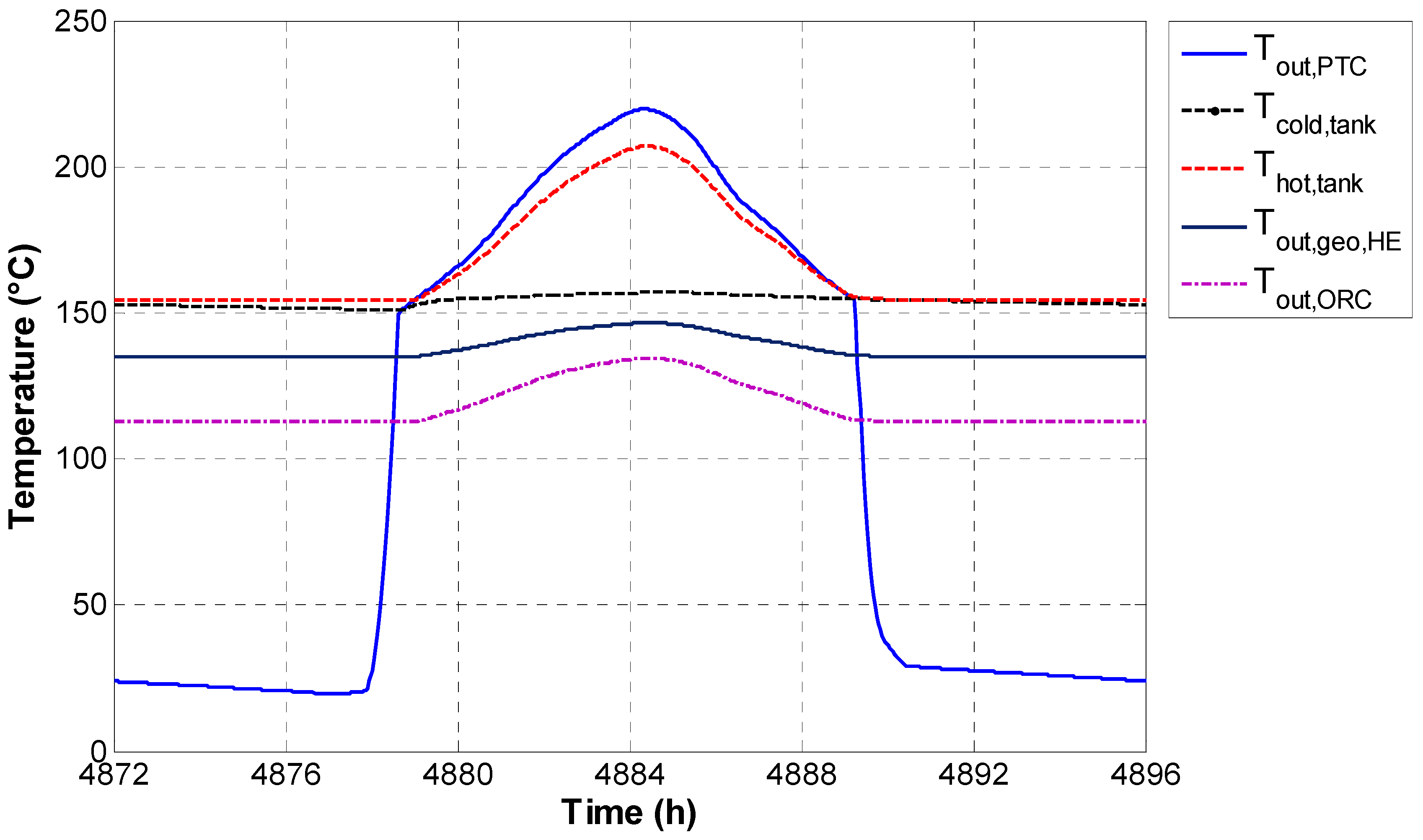
In order to investigate the trends of the investigated parameters during the year, a typical summer day, 23 July, has been selected. The parameters subsequently shown in this section are dramatically affected by the weather conditions. Varying the selected day, the trends are similar but the magnitude of the temperatures/powers may significantly vary. As typically occurs in summer period, it can be noted that there is a significant difference between night and day due to the solar gain. In fact, during the day higher temperatures are reached, as shown in
Figure 3. The PTC pump is activated in the early morning when the PTC outlet temperature (
Tout,PTC) becomes higher than the tank bottom temperature (
Tcold,tank). Then, the PTC loop continues to be activated until the late evening when it is stopped in order to prevent heat dissipation. Note that the solar loop is equipped with a fixed speed pump. Therefore, the PTC outlet temperature (
Tout,PTC) varies as a function of solar radiation availability. The maximum temperature reached by PTC (
Tout,PTC) on this day is 220 °C, while the one at the top of the tank (
Thot,tank) is 207 °C. Note that
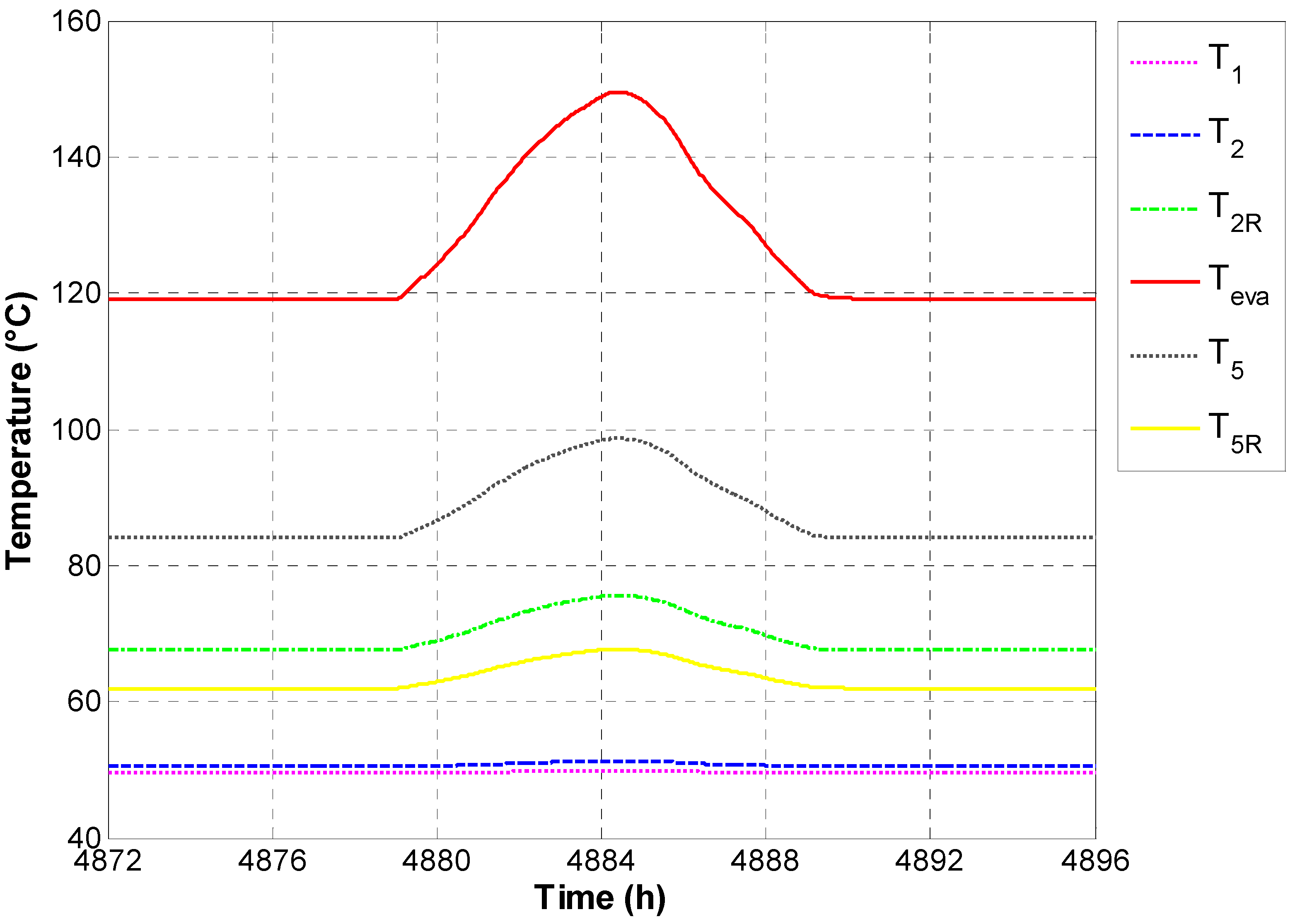
Thot,tank is also the temperature of the diathermic oil to be supplied to the ORC. As a consequence, during daytime the ORC driving temperature varies significantly. Therefore, solar radiation also determines a general increase of all the temperatures within the ORC cycle, as shown
Figure 4. The maximum evaporation temperature (
Teva equal to 150 °C) is achieved around midday. Such a figure also shows a significant variation of the evaporation temperature (
Teva) whereas the condensing temperature (
T1) shows only a slight increase. As a consequence, the evaporation pressure (
Peva) increases up to 16 bar, while the condensation one (
Pcond) does not significantly vary (not shown in Figures for brevity).
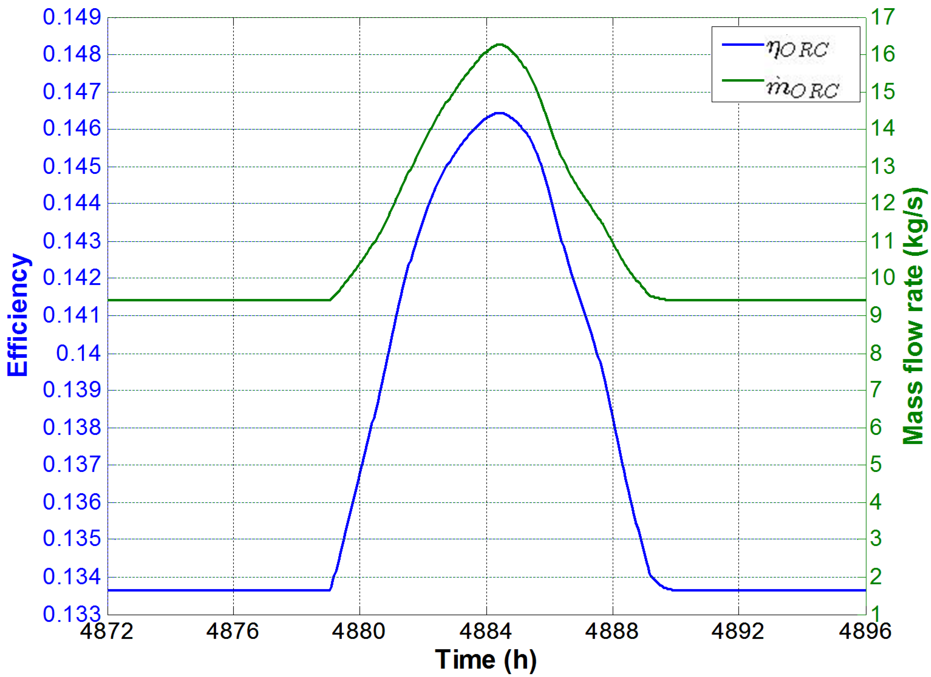
This determines a higher ORC efficiency (η
ORC) (
Figure 5), which reaches a maximum of 0.146.
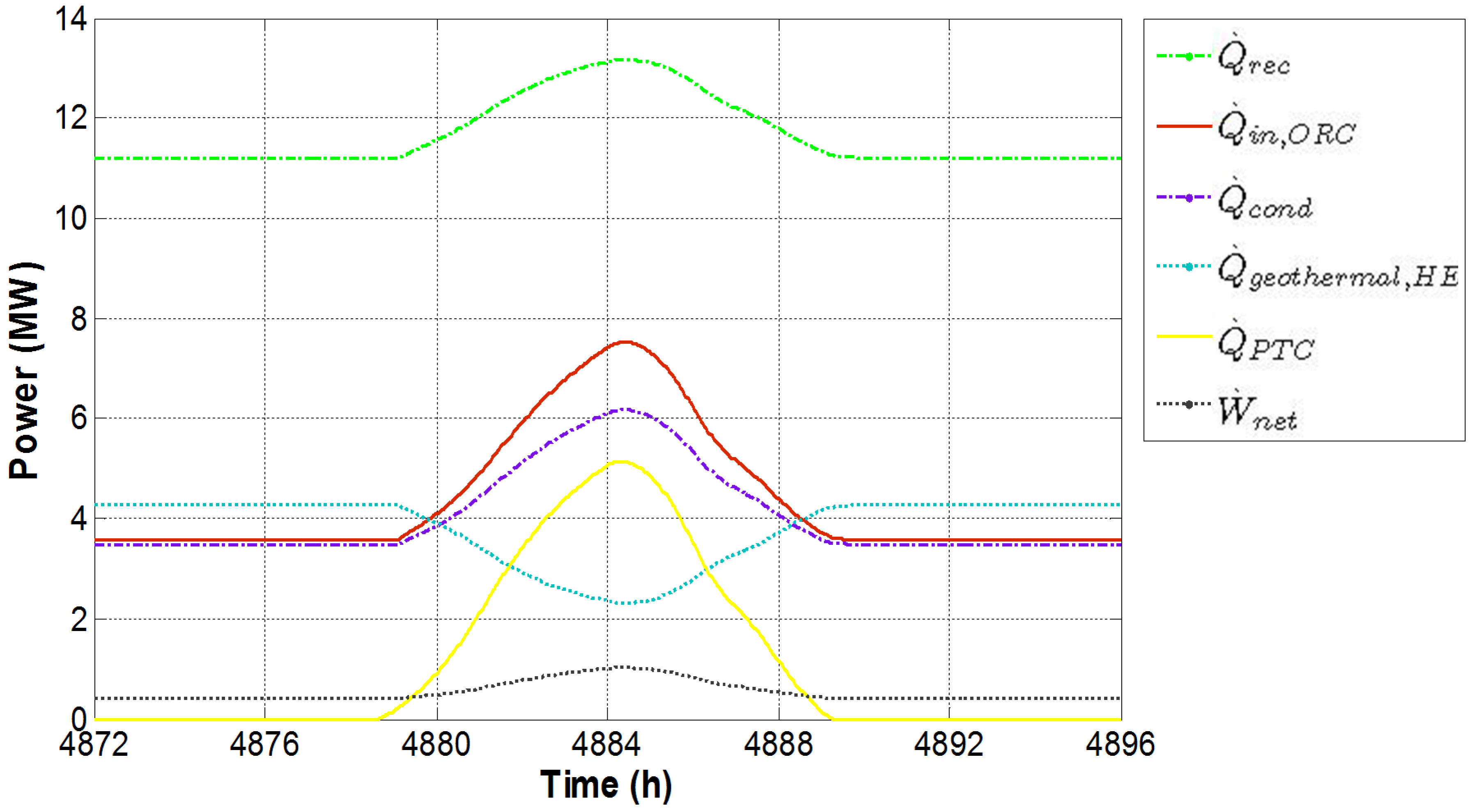
Figure 5 also shows that during the central hours of the day a significant increase of ORC mass flow rate is detected. In fact, as expected, the higher the temperature of the fluid entering the turbine, the higher the mass flow rate. As mentioned above, the net power produced by the plant is related both to the expansion ratio and mass flow rate. Therefore, the simultaneous increase of both expansion ratio and mass flow rate determines the increase in net power production, shown in
Figure 6, where a maximum net power of the whole plant (
) of 1.03 MW is obtained. It is worth noting that the net power also includes the electrical demands of Pump 1, Pump 2 and Pump 3. In
Figure 6, the higher contribution of solar energy is also clearly shown. PTC thermal power produced (
) achieves a peak of 5.14 MW determines a corresponding increase of thermal power supplied to the ORC (
). Consequently, the higher the ORC input thermal power, the higher the electrical and cogenerative (
) powers. During the night, thermal power supplied by the geothermal heat exchanger (
) is almost constant since the overall system operates very close to the steady state. Conversely, during daylight thermal capacity of geothermal HE (
) decreases (due to the higher oil inlet temperature), determining a corresponding increase of the heat recovered by the recuperator (
).
Figure 3.
Temperatures of the plant in a summer day.
Figure 3.
Temperatures of the plant in a summer day.
Figure 4.
ORC temperatures in a summer day.
Figure 4.
ORC temperatures in a summer day.
Figure 5.
Efficiency and mass flow rates in a summer day.
Figure 5.
Efficiency and mass flow rates in a summer day.
Figure 6.
Powers of system in a summer day.
Figure 6.
Powers of system in a summer day.
In
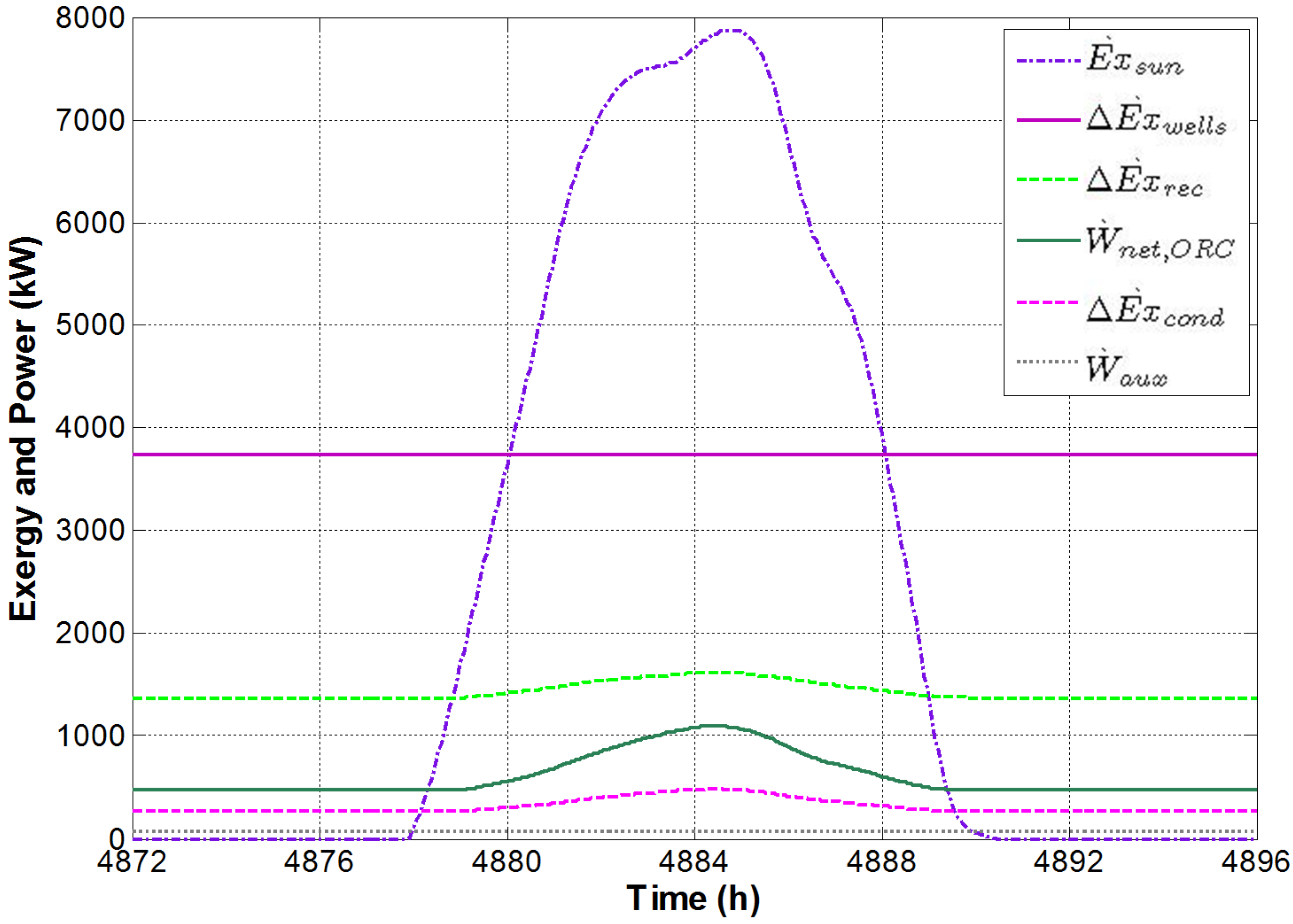
Figure 7, exergy flows for the selected summer day are shown. Here, a significant increase of the solar exergy flow (
) is detected during daylight, which reaches a maximum of 7.9 MW. This increase in the exergetic input (exergetic fuel) determines a general growth of all the exergy outputs, namely: exergy flows in the recuperator (
), condenser (
) and the ORC net power (
) (the corresponding maximums are respectively: 1,600 kW, 490 kW and 1,100 kW).
Figure 7.
Exergy flows in a summer day.
Figure 7.
Exergy flows in a summer day.
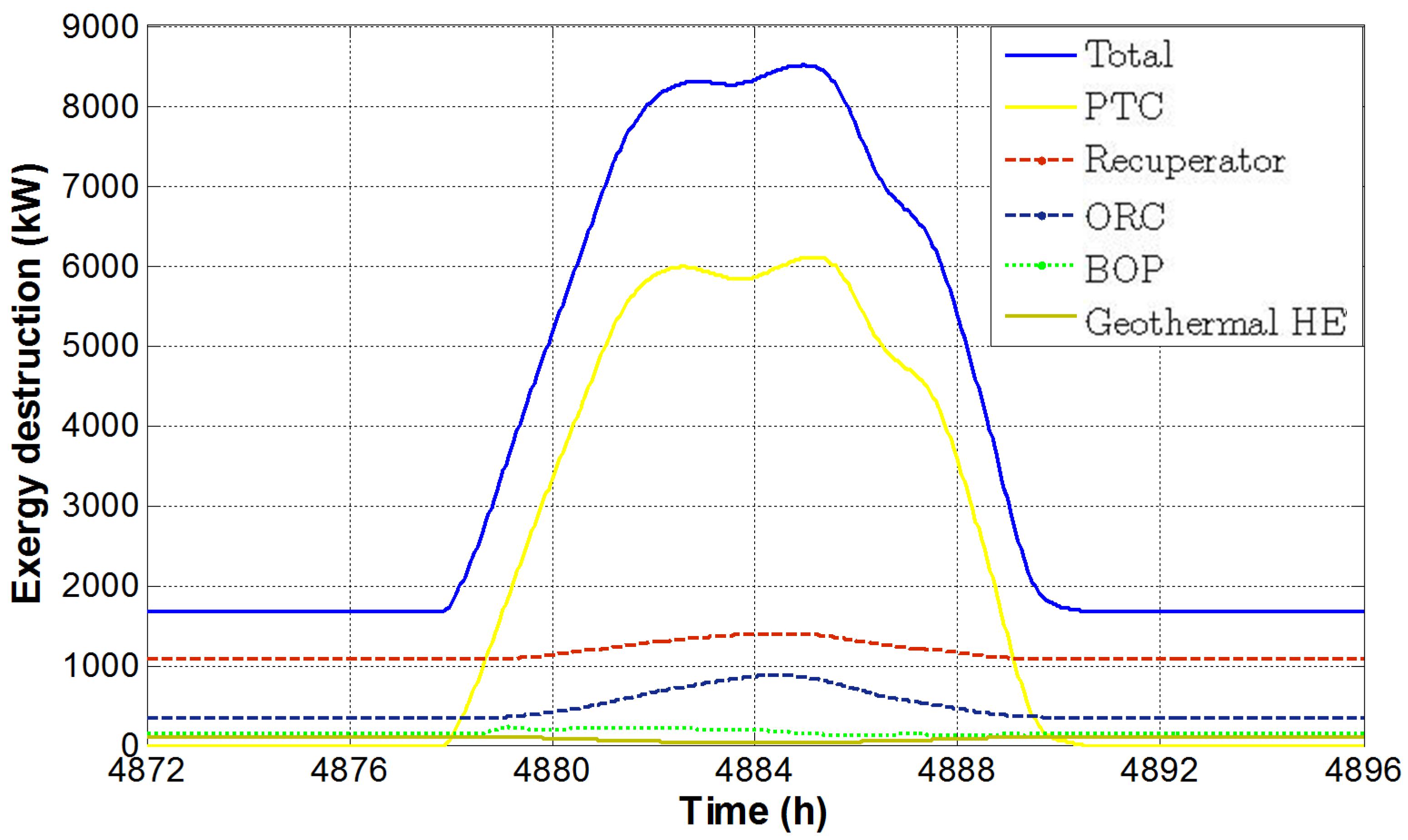
Figure 8 shows the exergy destructions of the system and its components. As expected, in accordance with the findings available in literature, the main contribution is again due to the PTC. A peak of 6.1 MW is achieved, when the total system exergy destruction rate is 8.5 MW. An increase in exergy destruction is detected also for the recuperator and the ORC (reaching a maximum of 1,400 kW and 880 kW, respectively) due to the increase of their capacities. The higher contribution of solar energy involves a lower heat exchange in the geothermal HE. Therefore, a smaller value of exergy destruction is achieved in this component equal to 27 kW during daytime. The exergy efficiencies are shown in
Figure 9.
Figure 8.
Exergy destructions in a summer day.
Figure 8.
Exergy destructions in a summer day.
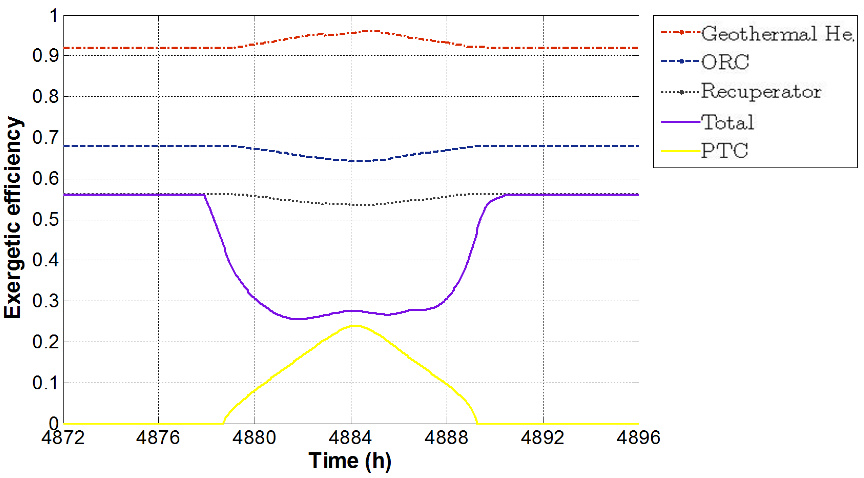
Figure 9.
Exergy efficiencies in a summer day.
Figure 9.
Exergy efficiencies in a summer day.
The high temperatures reached in the solar collectors allow one to achieve high exergetic efficiencies (conversely, PTC energetic efficiency, not shown in the Figure, decreases when its operating temperature is higher). In fact, the exergy efficiency increases when the temperature difference between the heat source (Tsun) and the fluid to be heated decreases, showing a maximum of 0.24. Conversely, when the PTC exergetic efficiency is defined by Equations (6) and (7), a much higher reading of such parameter is obtained (even higher than 60%) due to the lower temperature difference between the source (the plate of the collector) and the fluid to be heated. It is worth noting that for the calculation of exergy efficiency of the solar collector, although the approach based on Equations (3) and (5) is the most common selection in literature, the second alternative approach—Equations (6) and (7)—must be considered as the most appropriate one for the system under investigation which also includes geothermal energy. For that energy, input exergy is calculated using the exergy of the extracted geothermal brine, rather than the exergy related to the magma temperature. Therefore, for a suitable comparison, solar collector exergetic efficiency must be calculated with respect to the plate temperature rather than the solar surface temperature. As for the geothermal HE, the exergetic efficiency slightly increases during daytime, achieving a peak of 0.96, due to the lower temperature difference between the hot stream (geothermal brine) and the cold one (oil exiting from the ORC). Conversely, ORC and recuperator exergetic efficiencies slightly decrease during daytime, reaching a minimum of 0.64 and 0.54, respectively. Finally, the total exergetic efficiency of the system is the same shown in winter during the night. Conversely, the increase of solar radiation determines a decrease of the overall system exergetic efficiency, reaching a minimum (0.26) slightly lower than in the winter case.
4.2. Weekly Analysis
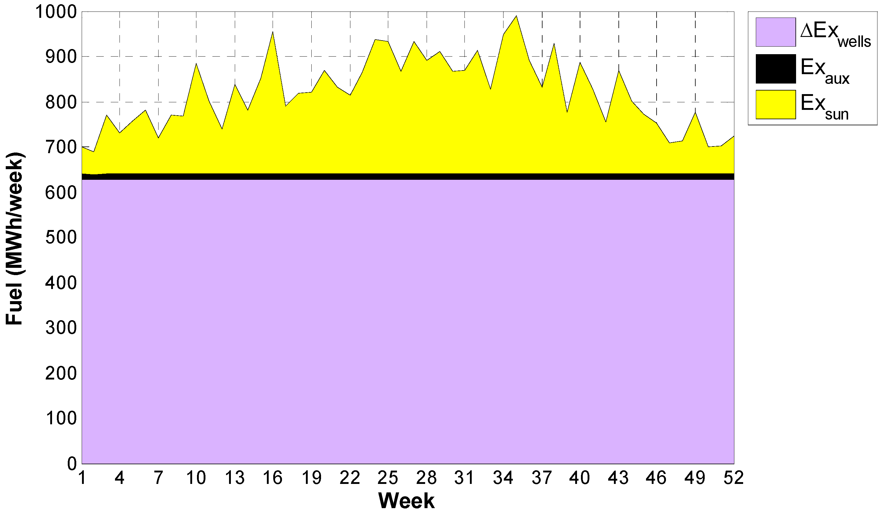
Results of the simulations are also integrated on a weekly basis in order to perform energetic and exergetic analyses of the system aiming at investigating performance parameters variations during the year. The weekly cumulated exergetic flows entering the system (exergetic fuels) are shown in
Figure 10. The contribution of the cumulated exergy associated to the geothermal source (ΔEx
wells) is dominant during the year. It is almost constant during the year around 628 MWh/week. The geothermal contribution is about from 63% to 91% of the overall exergetic fuel of the plant. Exergy related to the solar energy (Ex
sun) varies during the year, increasing during the summer. It ranges from 50 MWh/week obtained in the second week, to 350 MWh/week of the thirty-seventh week. The exergy associated to the auxiliary components (Ex
aux) is basically constant and negligible, being about 12 MWh/week.
Figure 10.
Weekly contribution of the different fuels.
Figure 10.
Weekly contribution of the different fuels.
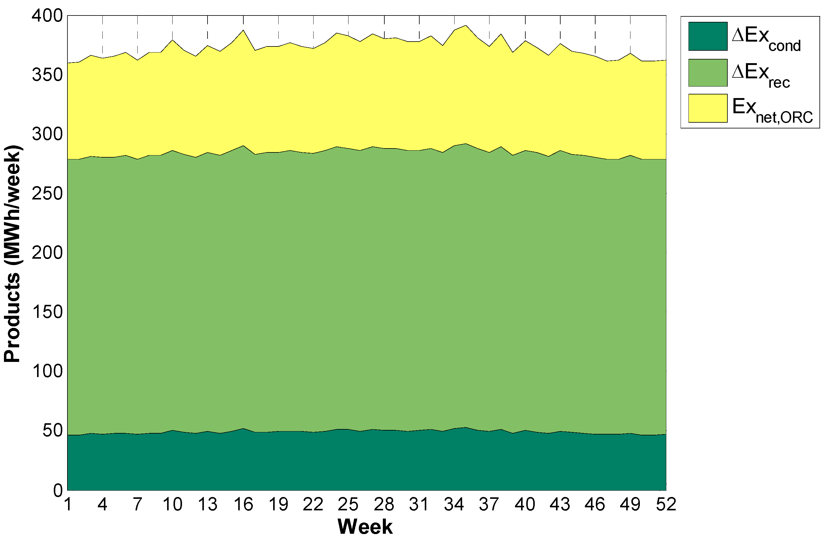
The exergies associated to the different exergetic products are shown in
Figure 11. This graph clearly shows that the highest one is due to the heat recovered by the recuperator (ΔEx
rec), ranging from 230 to 240 MWh/week, corresponding to a variation from 53% to 67% of the total exergy product. The exergy product related to the heat recovered by the condenser (ΔEx
cond) varies from 46 to 53 MWh/week, while the net exergy obtained in the ORC (Ex
net,ORC) ranges from 82 MWh/week of the first week to 100 MWh/week of the thirty-fifth week. This result shows that heat recovery from recuperator and condenser is crucial in order to reduce exergetic dissipations in the system.
Figure 11.
Weekly contribution of the different products.
Figure 11.
Weekly contribution of the different products.
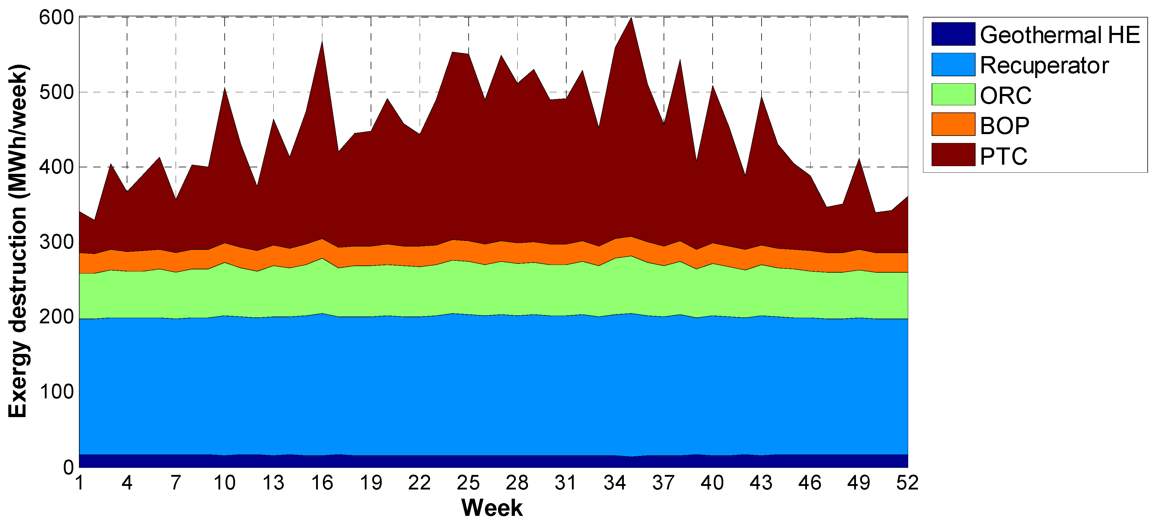
Components’ exergy destruction rates are shown in
Figure 12. As expected, the variability of solar energy availability determines a corresponding fluctuation of the exergy destroyed in the solar field. In fact, the exergy destruction in the PTC ranges from 45 MWh/week in winter to 290 MWh/week in summer, when it is 45% of the total destroyed exergy. Obviously, such variation is mainly due to the variation in its thermal capacity and efficiency. It is also worth noting that an increase in PTC exergy destruction also corresponds to an increase in ORC destruction rate. In fact, in such weeks the increase in PTC thermal capacity also determines an increase in ORC capacity, causing a corresponding growth of its exergy destruction rate. ORC exergy destruction varies from 61 to 75 MWh/week and affecting the total up to a maximum of 18%. Another important contribution to the overall exergy destruction rate is due to the recuperator. The exergy destruction in this component varies from 180 MWh/week in winter season to 190 MWh/week in the summer. It ranges from the 32% of the total in summer to the 55% in winter, when the solar contribution is very small. Geothermal HE and BOP exergy destructions are small, ranging from 14 to 17 MWh/week and from 26 to 28 MWh/week, respectively.
Figure 12.
Weekly contribution of the exergy destruction of the different components.
Figure 12.
Weekly contribution of the exergy destruction of the different components.
4.3. Annual Energetic, Exergetic and Economic Analyses
The annual performances of the system are reported in
Table 9. The energetic and exergetic analyses show that the contribution of the solar source is one order of magnitude lower than the geothermal energy one. In fact, in terms of energy, in a year the PTC produces 4.13 × 10
3 MWh compared to 35.7 × 10
3 MWh exchanged in the geothermal HE. In terms of exergy, instead, exergetic flow received from the Sun is equal to 9.4 × 10
3 MWh, compared to 32.7 × 10
3 MWh of geothermal exergy input. It is worth noting that the exergy destroyed in PTC is an order of magnitude higher than that destroyed in the geothermal HE, being respectively 8.0 × 10
3 MWh and 825 MWh. In fact, the solar thermal collectors operate subject to large temperature differences, (between the Sun temperature and the one of the fluid to be heated), causing large irreversibilities. Conversely, in geothermal HE, the temperature differences between the geothermal brine and diathermic oil are much lower, allowing one to achieve a better exergetic performance. Therefore, it is reasonable to expect that the values of exergetic efficiency in these components are significantly different. In fact, it is 14.94 for the PTC (
) and 92.40% for the geothermal HE (
). In addition, as expected, the exergetic efficiency calculated referring to the absorber plate temperatures rather than Tsun (
) is much higher than the previous one (
), being 41.53%. As shown by the previous figures, the system is dominated by the geothermal source. As a consequence, the calculated solar fraction is very low (10%).
Table 9.
Annual performance of the system.
Table 9.
Annual performance of the system.
| Parameter | Value |
|---|
| PTC thermal energy | 4126 MWh |
| Geothermal HE thermal energy | 35,736 MWh |
| Recuperator thermal energy | 99,894 MWh |
| ORC inlet thermal energy | 34,150 MWh |
| ORC net electric energy | 4,634 MWh |
| Condenser thermal energy | 32,475 MWh |
| Solar fraction | 0.1035 |
| Exergy associated to the solar source | 9,422 MWh |
| Exergy associated to the geothermal source | 32,727 MWh |
| Exergy associated to the recuperator | 12,247 MWh |
| Exergy associated to the condenser | 2,549 MWh |
| Exergy associated to the auxiliary components | 612 MWh |
| Exergy destruction in the PTC | 8,014 MWh |
| Exergy destruction in the geothermal HE | 825 MWh |
| Exergy destruction in the recuperator | 9,631 MWh |
| Exergy destruction in the ORC | 3,466 MWh |
| Exergy destruction in the BOP | 1,394 MWh |
| Total exergy destruction in the plant | 23,330 MWh |
| 0.1357 |
| 0.6959 |
| 0.1494 |
| 0.4153 |
| 0.9240 |
| 0.5598 |
| 0.4544 |
| PTC cost | 6,000,000 € |
| Wells cost | 800,000 € |
| Geothermal HE cost | 259,809 € |
| Recuperator cost | 270,000 € |
| ORC cost | 4,800,000 € |
| BOP cost | 652,981 € |
| Management and maintenance cost | 255,656 € |
| Electric energy produced revenue | 736,540 €/year |
| Thermal energy produced revenue | 6,883,192 €/year |
| SPB | 1.74 years |
Regarding the products, both in terms of energy (99.9 × 10³ MWh) and exergy (12.2 × 10³ MWh), the main contribution is due to the recuperator. The electric energy produced in a year is equal to 4.6 × 10³ MWh. It is important to notice that the value of the ORC energetic () and exergetic
efficiencies, respectively 13.57% and 69.59%, and the value of the exergetic efficiency of the whole system () equal to 45.44%.
The economic performance of the system is also evaluated. Economic analysis was performed on the basis of the results of the annual simulations, using the Simple Pay Back period (SPB) as objective function. As concerns system capital costs, they are dominated by PTC and ORC, being respectively 6 M€ and 4.8 M€. In fact the overall capital cost is 12.8 M€. Other costs to be reported are due to the geothermal wells and to the BOP, which are respectively 800 k€ and 650 k€. It is worth noting the costs related to the exploitation of geothermal resources are dramatically affected by the geographical location and by the overall depth of the geothermal well. In this study, as mentioned before, this cost has been estimated on the basis of a specific quote obtained by a local drilling company [
47]. Obviously, such costs may dramatically vary for alternative locations, especially when geothermal fluid is available at lower depths. The economic analysis also points out that the capital cost of the solar field is not proportional to its contribution in terms of electrical production. In fact, as mentioned before, about 47% of the total cost is due to the solar field whereas the solar fraction is slightly higher than 10%. This result shows that the hybridization of the geothermal-ORC system using solar collectors enhances its energetic performance. However, a significant increase of system capital costs must be taken into account.
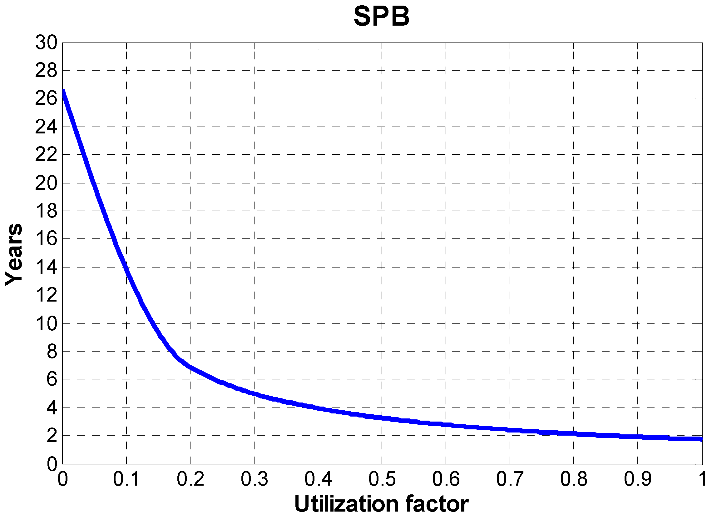
The revenues from the production of thermal energy (6.9 M€) are an order of magnitude higher than the ones related to the electricity (740 k€). This result is not surprising since system thermal production is much higher than the electrical one. However, in order to analyse the effect of this revenue on the overall economic performance, a sensitivity analysis is performed in order to calculate the variation of the SPB as a function of the rate of the utilization of the thermal energy produced by the system. This analysis is shown in
Figure 13: SPB varies from 26.6 years (no thermal energy demand) to 1.7 year (thermal energy fully utilized by the user). This shows that at full utilization of the heat from cogeneration, excellent economic performance can be obtained. Obviously, such circumstances can be achieved in case of large and constant demands of low-temperature heat (e.g., domestic hot water, low-temperature space heating,
etc.).
Figure 13.
SPB in function of the utilization factor of thermal energy.
Figure 13.
SPB in function of the utilization factor of thermal energy.
4.4. Parametric Analysis
A parametric analysis was also performed varying several parameters (such as collector area, tank volume, set point temperatures, etc.) and then evaluating the results from the energetic, exergetic and economic points of view. In all the parametric analyses, the capacities of the ORC and geothermal wells are kept constant since these parameters are strictly related to the geothermal capacity of the location. For sake of brevity, the following section presents the results of the analysis only with respect to the PTC area, being this parameter dominant over the remaining ones. In all the following parametric analyses, design parameters are varied in a large range centered on the initial value set in the previous sections. Such a range is determined considering the upper and lower limits corresponding to reasonable design conditions.
Collector Area
The PTC area is varied from 5,000 to 15,000 m
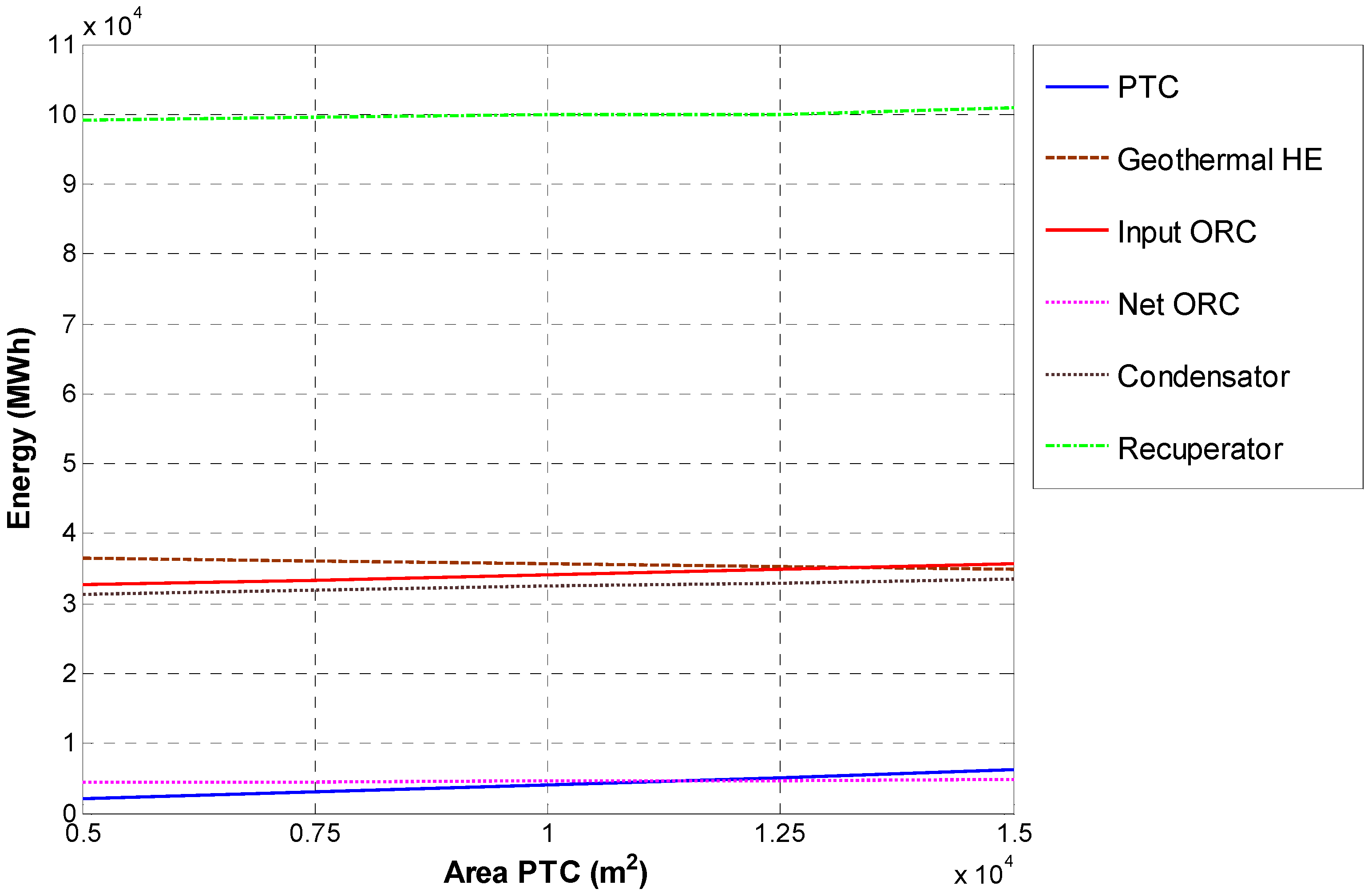
2. In such a large range, the rated solar thermal capacity varies approximately from 2.5 to 7.5 MW. Lower or higher PTC areas are not considered since in those cases the solar fraction would be dramatically low or high, respectively Annual thermal energies are shown in
Figure 14. Obviously, the PTC thermal energy increases in case of large solar fields, from 2,100 MWh (5,000 m
2) up to 6,200 MWh (15,000 m
2). For all the configurations, the PTC thermal energy is an order of magnitude lower than the one exchanged in geothermal HE, which decreases in the case of larger solar fields, as discussed in the previous sections. In fact, geothermal energy used for ORC varies from 36,500 MWh (5,000 m
2) to 35,000 MWh (15,000 m
2). The ORC inlet thermal energy ranges from 32,700 to 35,800 MWh, in case of larger solar fields. This increase involves also a growth of the net electric energy obtained by the ORC, ranging from 4,400 MWh up to 4,900 MWh. In addition, thermal energy recovered in the condenser and the recuperator increase, ranging, respectively, from 31,400 MWh up to 33,600 MWh and from 99,100 MWh up to 101,000 MWh.
Figure 14.
Thermal energy used and net electricity produced in a year varying collectors area.
Figure 14.
Thermal energy used and net electricity produced in a year varying collectors area.
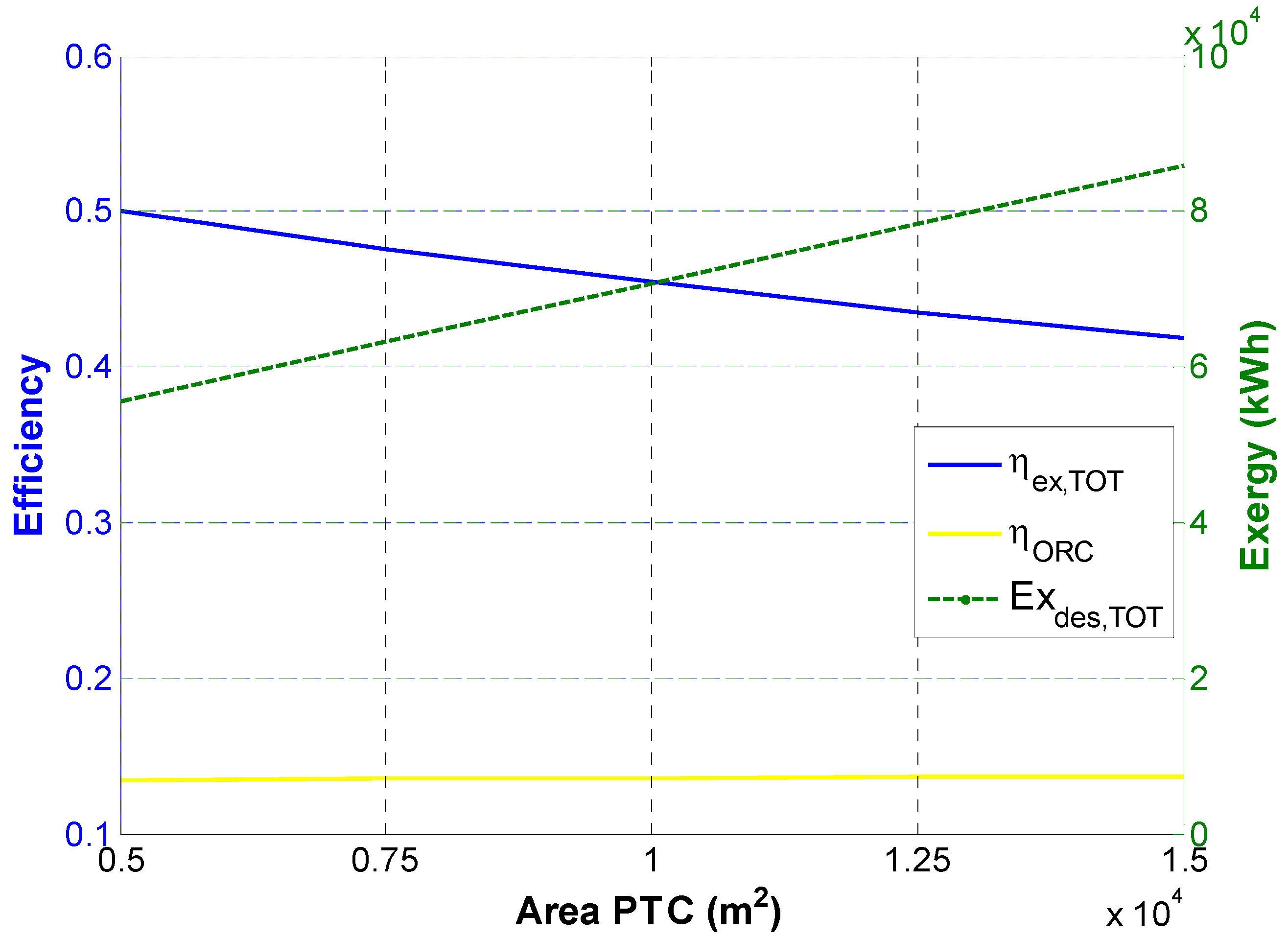
Figure 15 shows that a variation of PTC area significantly affects the system’s overall exergetic efficiency (η
ex,TOT) which ranges from 0.500 for the minimum collector area to 0.418 for the maximum one. Therefore, for a larger PTC area, exergy fuels increase more than exergy products. This is due to the fact that the larger the solar field, the higher the PTC temperature, determining a lower efficiency and therefore higher irreversibilities. Hence, the exergy destruction in the whole system (Ex
des,TOT) increases significantly, varying from 55.6 to 86.0 MWh, as shown in
Figure 15. This figure also shows that the ORC efficiency (η
ORC) is almost constant, ranging from 0.135 to 0.137. Therefore, in terms of energy, a slight increase of the products compared to the fuels has been obtained by the increasing collector area.
Figure 15.
Efficiencies and exergy destruction by varying the collector area.
Figure 15.
Efficiencies and exergy destruction by varying the collector area.
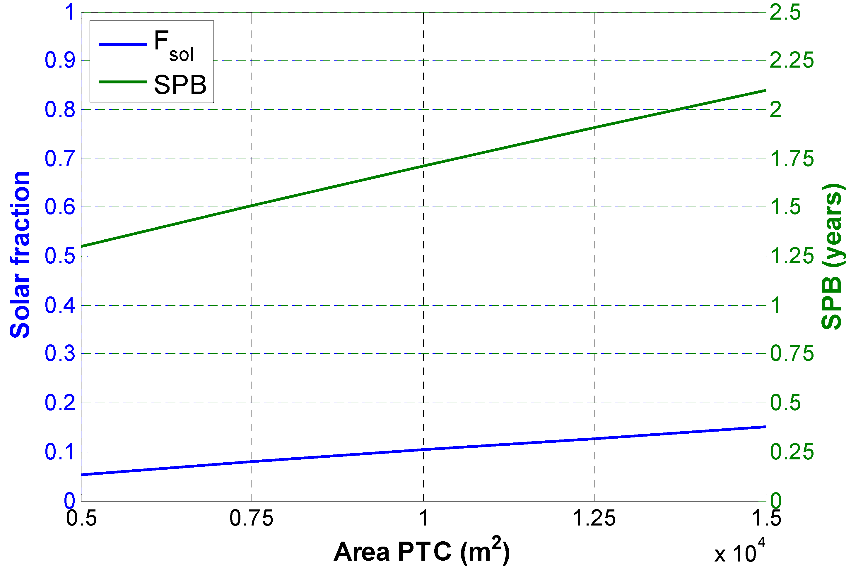
Figure 16 shows that both the solar fraction (
Fsol) and SPB increase for larger solar fields. As discussed above, an increase of the PTC area involves an increase of the energy produced by the PTC and a decrease of the energy exchanged in the geothermal HE. Therefore, the solar fraction increases for larger solar fields. For the considered range of variation of the PTC area, the solar fraction varies approximately from 5% to 15%. Therefore, smaller solar fields are not taken into account since their contribution to the overall energy production would be negligible. Conversely, larger solar fields are not feasible, since in those cases the system’s economic profitability decreases dramatically. In fact, the trend of the SPB shows a linear increase for larger solar fields. It is worth noting that, for the selected range of variation, a monotonic SPB trend is found and therefore, the minimum coincides with the lower limit. This is quite surprising since, from the economic point of view, two opposite trends must be considered in the case of solar fields: a higher capital cost and a higher electrical energy production. Such opposite trends should determine a non-monotonic trend of the SPB. Unfortunately, the minimum occurs very close to zero, corresponding to an extremely low solar fraction that suggests that, in those conditions, the hybridization does not make sense. As a consequence, this result suggests a better economic profitability of the geothermal source compared with the solar one.
Figure 16.
Solar fraction and SPB by varying the collector area.
Figure 16.
Solar fraction and SPB by varying the collector area.
4.5. Exergetic and Thermo-Economic Optimizations
Exergetic and economic optimizations have been also performed. The optimization is performed by simultaneously varying several design parameters in order to identify the minimum of a well-defined objective function. For this purpose, complex mathematical algorithms have been used thanks to the TRNOPT plug-in included in the TRNSYS package, which links the TRNSYS dynamic simulation to the optimization algorithm. The algorithms used have been developed by Lawrence Berkeley National Laboratory and are included in the GENOPT package. In particular, among the various proposed, the modified version of the Hooke–Jeeves algorithm [
50] has been selected. It allows a very efficient optimization, ensuring that a number of simulations compatible with reasonable computational times is ensured. In order to reduce this time, a relatively small number of variables has been considered. Namely, the variables considered in this study are the collector area (
APTC), the unitary volume tank and the diathermic oil mass flow rate circulating in the solar loop (
). The first variable varies in the same range used in the parametric analysis, the second between 0.005 and 0.015 m
3/m
2, and the last one between 20 and 60 kg/s. The initial conditions are the design ones discussed above. The objective functions are two: the total exergy destruction (Ex
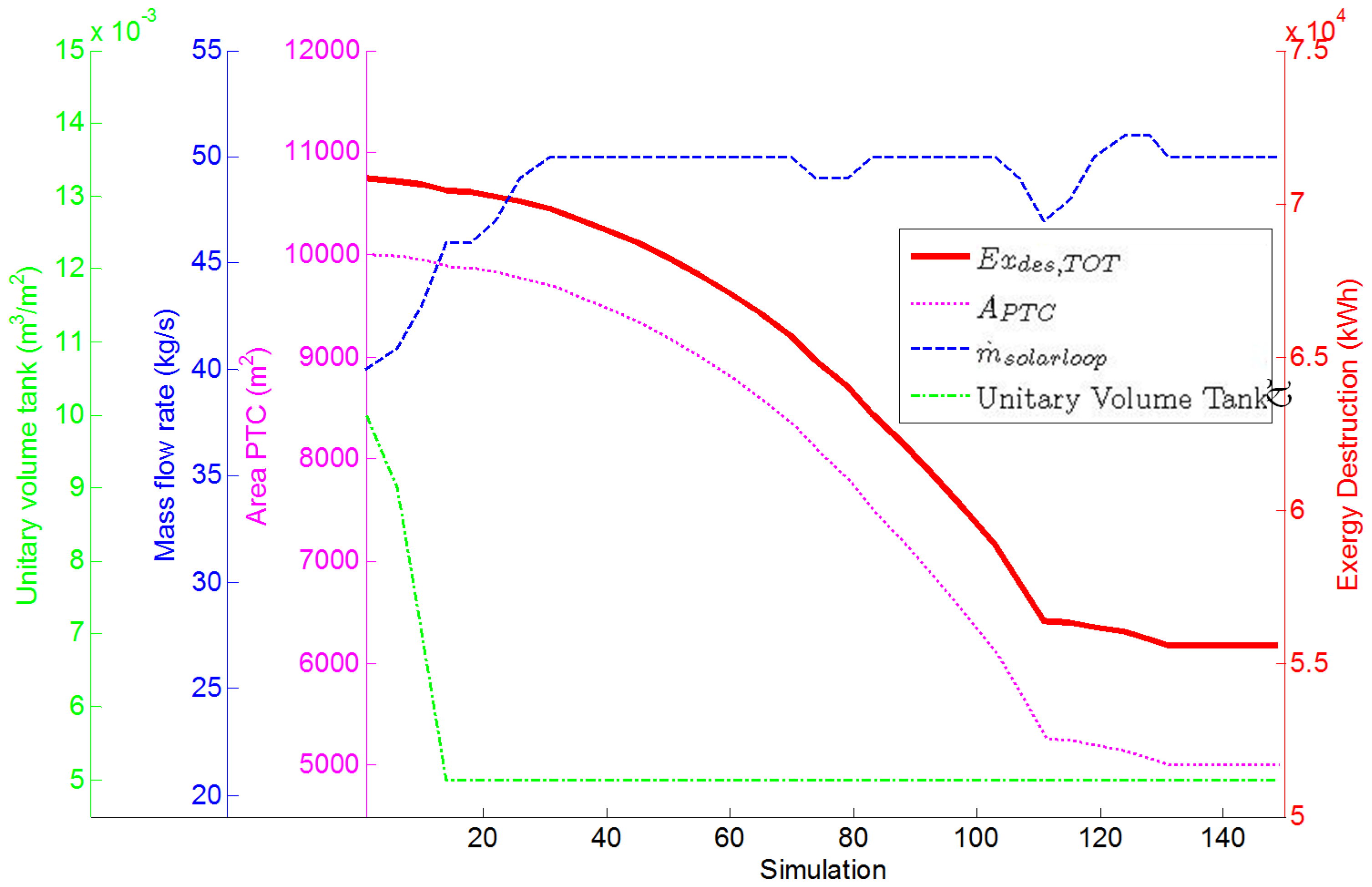
des,TOT) and the SPB. Obviously, the target is to minimize such functions. The results are shown in
Figure 17 and
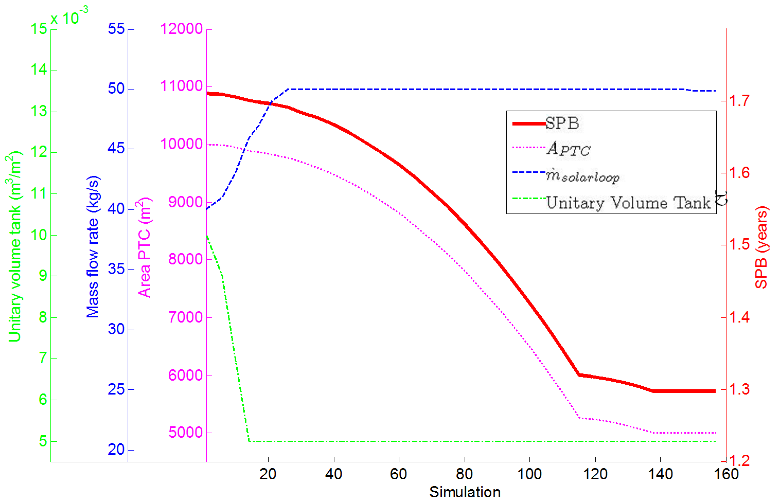
Figure 18. These figures show, for each iteration of the optimization procedures, the values of the objective functions and the ones of the design variables. As a consequence, the optimum is found for the last iteration of the optimization procedure. Here, the optimal values of the design variable, and the corresponding readings of the objective functions can be read.
The convergences are achieved after 149 simulations in the first case and after 157 in the second. In such configuration, respectively the best exergetic and economic performance of the plant are achieved. It is worth noting that both objective functions are minimized for the same values of the variables considered. Furthermore, it should be emphasized that the results of the optimization are consistent with the ones obtained by the parametric analysis. In fact, in accordance with the findings shown in
Section 4.4, the minimum values of the total exergy destruction and of the SPB are achieved for the minimum solar collector area.
Figure 17.
Optimization of the plant using the total exergy destruction as objective function.
Figure 17.
Optimization of the plant using the total exergy destruction as objective function.
Figure 18.
Optimization of the plant using the SPB as objective function.
Figure 18.
Optimization of the plant using the SPB as objective function.
The optimum is similarly obtained for the minimum tank volume and for the maximum solar loop flow rate. Similar results are obtained by the corresponding parametric analyses (not shown in the paper for sake of brevity). In addition, the values of the total exergy destruction and the SPB achieved are 55,600 kWh and 1.3 years, the same values obtained in the parametric analysis using the minimum collector area value.
In fact, as previously discussed, the total exergy destroyed decreases with collector area, because the exergy products increase less than the exergy fuels with a larger PTC area. On the other hand, system exergetic efficiency is significantly affected by the capacity of the solar field. In fact, repeating the optimization using system exergetic efficiency as objective function (not shown in the Figures for brevity), the optimal configuration was found when collectors area is equal to 5,000 m2, improving the exergetic efficiency from 0.45 to 0.50.
Regarding the SPB, it is worth noting that the PTC cost has a very high influence on the total cost of the system. Therefore, a collector area increase does not involve an appropriate increase in revenues due to the higher electricity generated and heat energy obtained.
In both optimizations, the unitary volume tank achieves its minimum value. Note that smaller tank capacities are not taken into account since 0.005 m3/m2 is considered the smallest size in order to achieve a suitable hydraulic separation between ORC and solar loops. For lower tank capacities, severe turbulences in pump operation could be achieved. However, the variation of tank volume only slightly affects the objective functions under consideration, as discussed above. However, the optimal configuration is found for the minimum value volume of the tank. In fact, its increase leads to an increment of the thermal losses to the environment. Conversely, the relative amount of thermal losses decreases due to the smaller surface to volume ratio achieved in the case of larger tanks. Furthermore, it is worth noting that thermal losses (and exergy losses) can be reduced by increasing tank insulation. Therefore, the total exergy destroyed increases with the increase of the tank volume. From the economic point of view, using larger tanks is never profitable. In fact, the capital cost is higher and the overall energy production is lower. Therefore, SPB increases for larger tank volumes. Thus, it can be concluded that the tank must act only as hydraulic separator between the solar loop and the ORC loop.
Finally, in both optimizations, the optimal value of the diathermic oil mass flow rate of the solar loop is 50 kg/s. As mentioned above its variation also slightly affects the total exergy destruction and the SPB.
5. Conclusions
A simulation model of a solar-geothermal hybrid cogeneration plant that uses an Organic Rankine Cycle (ORC) has been developed. The system uses a medium-enthalpy geothermal resource and a PTC field to exploit solar energy. Once the layout of the system is analyzed, the ORC model has been described in detail. It has been developed using zero-dimensional energy and mass balances with Engineering Equation Solver (EES) and it allows one to evaluate system performance in off-design conditions. Subsequently, the ORC simulation model has been implemented in a TRNSYS project in order to perform a dynamic simulation of the system. All the other components (PTC, geothermal well, heat exchangers, pumps, storage tank, controllers, etc.) have been added in order to perform energetic, exergetic and economic analyses. For this purpose, daily, weekly and annual simulations have been performed.
The solar gain allows one to achieve higher temperatures, pressures and mass flow rates for each state point of the ORC system, determining an increase of energetic efficiency, net power and thermal power recovered in the condenser and in the recuperator. In this circumstance, the thermal power exchanged in the geothermal HE decreases, due to the higher ORC outlet temperature from its primary heat exchanger. The exergetic analysis shows that the increase of exergy due to solar power allows one to increase the exergy of the water circulating through the recuperator and in the condenser and the net power produced by the ORC. The contribution of exergy due to the geothermal well is constant, as well as the power used by the auxiliary, which is also negligible. Furthermore, the main contribution to the exergy destruction is provided by PTC when there is solar availability. Otherwise, the recuperator is the source of the largest exergy destruction. Instead, in the geothermal HE and in the BOP exergy destruction is much lower than PTC one. Finally, the exergy efficiencies have been analyzed. It is well-known that the higher the amount of irreversibilities in the component, the lower the efficiency. Therefore, the trends observed are opposite to those of the exergy destructions.
Weekly simulations show that, among the fuels, the contribution of the exergy associated to the geothermal source is constant and preponderant during the year. Instead, among the products, the highest exergy flow is due to the heat recovered by the recuperator. The most significant change regarding the exergy destruction occurs in the PTC, which is maximum in summer. Another important contribution is due to the recuperator, especially in winter.
Annual simulations have been performed in order to realize an economic analysis of the system. After a detailed description of the economic model, the cost of each component has been analyzed. The main contribution to the total cost of the plant is due to the PTC and the ORC. In addition, different revenues were analyzed. Thermal energy produced is crucial in order to achieve good economic profitability. Indeed, in the case of a full utilization of cogenerative heat, the system shows excellent economic performance.
In addition, a parametric analysis has been performed varying collector area and volume tank. An increase of PTC area determines a corresponding growth of the thermal energy produced by the collectors and supplied to the ORC. Therefore, the ORC electrical production increases as well. Conversely, a decrease of the thermal energy exchanged in the geothermal HE has been detected. The ORC energetic and total exergetic efficiencies are constant regardless of the area of the collectors. Exergy destruction, solar fraction and SPB increase for larger of PTC solar fields.
The variation in tank volume, instead, negligibly affects the parameters mentioned above.
Finally, an optimization procedure has been performed in order to identify the plant configuration that allows one to achieve the best exergetic and economic performance. The results show that the objective functions (the total exergy destruction and the SPB) are minimized for minimum values of the collector area and the volume tank (per unit PTC area) and for a diathermic oil mass flow rate circulating in the solar loop of 50 kg/s.
The overall result of this analysis is that the hybrid layout, including simultaneously solar and geothermal energy powering an ORC cycle, is very profitable from the energetic point of view since the combination of solar field and the geothermal source allows one to increase both the electrical and thermal energy productions with respect to a conventional geothermal power plant. However, from both exergetic and economic points of view, such hybridization is not always convenient. In fact, the overall system exergy efficiency decreases when the solar field is added. The exergetic efficiency of the solar collector is dramatically low, determining an overall decrease of plant exergetic efficiency. However, the exergetic efficiency is not the most appropriate measure of the feasibility of the system since solar energy is not subject to any charge. Conversely, the study proved the feasibility of using PTC collectors to drive the ORC at the required operating temperatures. In addition, the economic criterion is a more appropriate measure to determine the feasibility of the hybridization of the geothermal ORC plant. From this point of view, the present capital cost of solar thermal collectors makes the hybrid system less profitable than a conventional geothermal-ORC power plant. This is due to a plurality of factors: (i) the capital cost of solar thermal collectors is very high; (ii) the operating time of solar thermal collectors is much lower than the one of the geothermal source; (iii) the increase of ORC supply temperature determines a significant enhancement of its electrical capacity but only a slight improvement of its electrical efficiency. However, such a scenario may vary significantly in the near future where a significant decrease of solar collector capital cost (for example, using Fresnel collectors) and a corresponding increase of fossil fuel costs are expected, determining a possible improvement of the profitability of the investigated hybrid system. Simultaneously, future works will aim at investigating some possible modifications in the layout of the hybrid system (double-pressure ORC, special storage systems, etc.) which may be used in order to improve the profitability of the solar subsystem.


