An Improved Artificial Bee Colony Algorithm and Its Application to Multi-Objective Optimal Power Flow

Abstract

Optimal power flow (OPF) objective functions involve minimization of the total fuel costs of generating units, minimization of atmospheric pollutant emissions, minimization of active power losses and minimization of voltage deviations. In this paper, a fuzzy multi-objective OPF model is established by the fuzzy membership functions and the fuzzy satisfaction-maximizing method. The improved artificial bee colony (IABC) algorithm is applied to solve the model. In the IABC algorithm, the mutation and crossover operations of a differential evolution algorithm are utilized to generate new solutions to improve exploitation capacity; tent chaos mapping is utilized to generate initial swarms, reference mutation solutions and the reference dimensions of crossover operations to improve swarm diversity. The proposed method is applied to multi-objective OPF problems in IEEE 30-bus, IEEE 57-bus and IEEE 300-bus test systems. The results are compared with those obtained by other algorithms, which demonstrates the effectiveness and superiority of the IABC algorithm, and how the optimal scheme obtained by the proposed model can make systems more economical and stable.

1. Introduction

Research on the optimal operation theory of power systems reached a new level after the optimal power flow (OPF) concept was proposed by the French scholar Carpentier in the 1960s [1,2]. OPF is regarded as a development and extension of the class power flow, and it can combine economic operations with safe operations, and active power optimization with reactive power optimization of power systems. It has been an effective optimization tool for power systems after further research by numerous academics.

The OPF problem is considered a complex multi-constraint, non-linear and non-continuous optimization problem. The linear programming [3,4], quadratic programming [5], simplified gradient method [6], Newton method [7] and interior point method [8] have been widely applied to solve it. These algorithms have relatively rapid calculation and are suitable for online calculation, but they aren’t suitable for optimization problems with discrete variables, as the optimization results are closely related to the position of initial points, so the algorithms easily converge to a local optimum when the position of the initial points is within the convergence domain of local optimum points.

Heuristic algorithms are novel algorithms for solving the OPF problem. Typical heuristic methods include the genetic algorithm (GA) [9,10], particle swarm optimization (PSO) [11,12] and others. These algorithms possess better global search abilities, aren’t restricted by the initial point position, and can effectively solve problems with discrete variables. However, the GA easily converges to local optima and has complex encoding and decoding operations. The PSO algorithm also has the premature ending phenomenon, and the convergence speed is slow the during later evolution periods.

The artificial bee colony (ABC) algorithm is one of the recently proposed heuristic algorithms, first suggested by Karaboga in 2005. It simulates the intelligent foraging behavior of honeybee swarms [13]. Its advantages include easy implementation and better exploration capacity, and it has been successfully applied to solve all kinds of optimization problems. The optimization mechanism of the ABC algorithm was analyzed in [14], performance testing was done using some typical numerical functions, and the results demonstrated that the ABC algorithm possesses superior performance in terms of solving numerical optimization problems compared with the GA algorithm, PSO algorithm and DE algorithm. In [15], the ABC algorithm was applied to solve an optimal reactive power flow problem of which the optimization objective was minimization of active power loss, and the simulation showed that the active power loss obtained by the ABC algorithm is lower than those obtained by other heuristic algorithms, and ABC algorithm had better convergence properties. In [16], the ABC algorithm was applied to solve a power system reconfiguration problem, which considered the active power loss as the objective function, and the simulation results showed that the power loss obtained by the ABC algorithm was less and the running time shorter than with other algorithms. In [17], the ABC algorithm was utilized to solve the economic dispatch problem, and the results indicated that the exploration capacity of the ABC algorithm was better than that of other algorithms. However, the ABC algorithm needs to further improve the capacities of maintaining population diversity and exploitation [18,19].

The paper proposes an improved ABC algorithm (IABC), and the search operation of the IABC algorithm for new solutions is replaced with the mutation and crossover operations of the DE algorithm to improve the exploitation capacity; the initial swarms, the reference solutions of the mutation operation and the reference dimensions of the crossover operation are generated by tent chaos mapping to improve the swarm diversity. The proposed IABC algorithm is applied to solve the multi-objective OPF problem of which the objective functions involve minimization of total fuel costs, minimization of emissions, minimization of active power losses and minimization of voltage deviations. The objectives are fuzzified by the fuzzy membership functions and the fuzzy satisfaction-maximizing method. The calculation model of the fuzzy multi-objective OPF-based IABC algorithm is established. Finally the proposed approach is tested on the standard IEEE 30-bus, IEEE 57-bus and IEEE 300-bus test systems. The results are compared with those obtained by other methods and demonstrate that the proposed approach is efficient and superior.

2. Optimal Power Flow Problem Formulation

The goal of OPF is to optimize objective functions by determining the optimal control variables while satisfying all the constraints. It can be formulated as:

Minimize: f_i(x,u) I = 1,2…, N_obj

(1)

Subject to: g(x,u) = 0, h(x,u) ≤ 0

(2)

where f_i is the objective function i; N_obj is the number of objective functions; g is the equality constraint; and h is the inequality constraint; x is the vector of dependent variables including slack bus generated active power, generator reactive power output, load bus voltage and transmission line flow; u is the vector of independent control variables including generator active power output, generator bus voltage, transformer tap settings and shunt VAR compensation. In this paper, four different objective functions are considered. Their mathematical models and OPF constraints are described as follows.

2.1. OPF Objective Function

2.1.1. Minimization of Total Fuel Cost

Nowadays with the rise in fuel prices and the increased power loads, the generated costs will obviously increase, therefore, it is important to find an optimal operation scheme to generate electricity with minimum costs by OPF calculation. The total fuel costs are considered one of the objective functions, and can be expressed as:

$$f_1={\displaystyle \sum _{i=1}^{N_{gen}}{a}_i{P_{Gi}}^2+b_i{P}_{Gi}+c_i}$$

(3)

where f₁ is the total fuel cost; N_gen is the number of generators; a_i, b_i, c_i are the fuel cost coefficients of the ith generator; P_Gi is the active power output of thermal unit i.

2.1.2. Minimization of Total Emission

These days due to the increasingly serious problem of air pollution, more and more countries are concerned about environmental protection. Therefore, it is necessary to reduce the emissions of atmospheric pollutants caused by the operation of fossil-fueled thermal generation facilities. The total emissions are also considered as one of objective functions, and can be described as:

$$f_2={\displaystyle \sum _{i=1}^{N_{gen}}{\text{α}}_i{P_{Gi}}^2+{\text{β}}_i{P}_{Gi}+{\text{γ}}_i}$$

(4)

where f₂ is the total emission; α_i, β_i, γ_i are the emission coefficients of the ith generator.

2.1.3. Minimization of Total Power Loss

Active power losses will occur during the operation of power systems, and more active power losses produced will increase the generated power costs. Therefore, the total power losses are also considered as one of the objective functions, and can be expressed as:

$$f_3={\displaystyle \sum _{i,j=1}^{N_{nod}}{G}_{ij}\left({V_i}^2+{V_j}^2-2V_i{V}_j\text{cos}{\text{θ}}_{ij}\right)}$$

(5)

where f₃ is the total active power loss; N_nod is total number of nodes; V_i, V_j are the voltage magnitudes at bus i and bus j, respectively; G_ij, θ_ij are the branch conductance and phase angles difference between bus i and bus j, respectively.

2.1.4. Minimization of Voltage Deviation

Bus voltage is one of the most important indices for secure operation and voltage quality. The objectives without voltage indices may result in a feasible solution that has an unattractive voltage profile [12]. Therefore, the load bus (PQ nodes) voltage deviations from 1.0 per unit are also considered as one of the objective functions, and can be expressed as:

$$f_4={\displaystyle \sum _{i=1}^{N_{PQ}}|V_i-1.0|}$$

(6)

where f₄ is the total voltage deviation; N_PQ is total number of PQ nodes; and 1.0 is per unit.

2.2. OPF Constraints

The OPF constraints include equality and inequality constraints. The equality constraints are the power flow equations, and they can be described as:

$$P_{Gi}-P_{Li}-V_i{\displaystyle \sum _{j=1}^N{V}_j\left(G_{ij}\cdot \text{cos }{\text{θ}}_{ij}+B_{ij}\cdot \text{sin }{\text{θ}}_{ij}\right)=0}$$

(7)

$$Q_{Gi}-Q_{Li}-V_i{\displaystyle \sum _{j=1}^N{V}_j\left(G_{ij}\cdot \text{sin }{\text{θ}}_{ij}-B_{ij}\cdot \text{cos }{\text{θ}}_{ij}\right)=0}$$

(8)

where P_Gi, Q_Gi are the active and reactive power output of the generating units at bus i, respectively; P_Li, Q_Li are the demanded active power and reactive power of loads at bus i, respectively; G_ij, B_ij, θ_ij are the transfer conductance, susceptance and voltage angle difference between bus i and bus j, respectively. In the OPF problem, the inequality constraints include:

(a)

Generator constraints: generator bus voltages, active power outputs, and reactive power outputs are restricted by their upper and lower limits as:

$$V_{Gi}^{\min }\le V_{Gi}\le V_{Gi}^{\max },i=1,2,\dots ,N_{gen}$$

(9)

$$P_{Gi}^{\min }\le P_{Gi}\le P_{Gi}^{\max },i=1,2,\dots ,N_{gen}$$

(10)

$$Q_{Gi}^{\min }\le Q_{Gi}\le Q_{Gi}^{\max },i=1,2,\dots ,N_{gen}$$

(11)

(b)

Transformer constraints: transformer tap settings are restricted by their upper and lower limits as:

$$T_{Tj}^{\min }\le T_{Tj}\le T_{Tj}^{\max },j=1,2,\dots ,N_{tra}$$

(12)

(c)

Shunt VAR constraints: shunt VAR compensations are restricted by their upper and lower limits as:

$$Q_{Ck}^{\min }\le Q_{Ck}\le Q_{Ck}^{\max },k=1,2,\dots ,N_{var}$$

(13)

(d)

Security constraints: these include the constraints of the load bus voltage magnitudes and transmission line loadings as:

$$V_{Dm}^{\min }\le V_{Dm}\le V_{Dm}^{\max },m=1,2,\dots ,N_{PQ}$$

(14)

$$S_{Ln}<S_{Ln}^{\max },n=1,2,\dots ,N_{lin}$$

(15)

3. Fuzzy Multi-Objective OPF Model

The paper considers the total fuel cost of generating units, the emission of atmospheric pollutants, the active power losses and the voltage deviations as the optimization objective functions. The methods for solving the multi-objective optimization problem include the weighting method [20] and fuzzy mathematics method [21]. The weighting coefficients of the weighting method are determined by decision maker preferences or several simulations. The fuzzy mathematics method utilizes membership functions to fuzzify the objective functions without weighting coefficient settings. In other words, the fuzzy mathematics method can make optimization results more objective and reasonable compared with the weighting method. We therefore utilize the fuzzy mathematics method to solve the multi-objective OPF problem, and use the following linear membership function so as to modify the candidate objective functions to its fuzzy form:

$$\mathrm{\mu }(f_i)=\{\begin{array}{ll}1& f_i\le {\mathrm{\lambda }}_{i\min }\\ \frac{{\mathrm{\lambda }}_{i\max }-f_i}{{\mathrm{\lambda }}_{i\max }-{\mathrm{\lambda }}_{i\min }}& {\mathrm{\lambda }}_{i\min }<f_i<{\mathrm{\lambda }}_{i\max }& i=1,2\mathrm{...},m\\ 0& f_i\ge {\mathrm{\lambda }}_{i\max }\end{array}$$

(16)

where f_i is ith objective function; µ(f_i) is the membership function of f_i; λ_imax is upper limit value of f_i and its value is the initial value; λ_imin is lower limit value of f_i and its value is obtained by the single objective optimization; m is the number of objective functions. The curves of membership functions given by the Equation (16) are shown in Figure 1.

The fuzzy satisfaction-maximizing method [22,23] is used to convert the multi membership function µ(f_i) into the objective function µ_F of fuzzy multi-objective OPF, and it can be expressed as:

$${\mathrm{\mu }}_F=\max \left\{1-\mathrm{\mu }(f_i)\right\}$$

(17)

Figure 1. Membership functions of each optimization objective.

Figure 1. Membership functions of each optimization objective.

The obtained model of fuzzy multi-objective OPF is described as:

Minimize: μ_F

(18)

Subject to: g(x) = 0, h(x) ≤ 0

(19)

The smaller value µ_F that is obtained by the fuzzy multi-objective OPF described by Equation (18) represents the higher fuzzy satisfaction value and the better optimal scheme.

4. Improved Artificial Bee Colony Algorithm

4.1. Artificial Bee Colony Algorithm

The artificial bee colony algorithm is a novel heuristic algorithm inspired by the behavior of honeybee swarms searching for food sources, and the process of searching for an optimal solution simulates the behavior of honeybee swarms foraging for food sources with a maximum nectar amount. A food source foraged by honeybees represents a feasible solution of the optimization problem, and the ith food source is described as X_i = (x_i1, x_i2,…, x_iD), where D is the number of dimensions for the optimization problem. The nectar amount of the food source represents the fitness value of the associated feasible solution [13,14]. The honeybee swarms are divided into employed bees, onlooker bees and scout bees, and their numbers are N_e, N_o and N_c, respectively. In the ABC optimization process, the employed bees do global searching for new food sources and pass on the information about the nectar amount to the onlooker bees; the onlooker bees choose one employed bee by the roulette wheel selection and do local searching for a new food source around the chosen one; if a food source isn’t improved by a predetermined number limit of trials, then that food source will be abandoned by the employed bee, and the scout bee will randomly generate a new food source instead of the abandoned one, therefore, this step can effectively avoid local optima. The optimization process of the algorithm mainly includes initialization, employed bee phase, onlooker bee phase and scout bee phase.

4.1.1. Initialization

The ABC algorithm randomly generates N_s numbers of initial feasible solutions X_i, generated as:

$$x_{ij}=x_{ij\min }+\text{rand}\times (x_{ij\max }-x_{ij\min })$$

(20)

where j = 1,2,…, D; x_ij is the jth dimension parameter of a feasible solution X_i; x_ijmax, x_ijmin are the upper and lower bounds for the dimension j, respectively; rand is random number between 0 and 1.

4.1.2. Employed Bee Phase

In the employed bee phase, the algorithm randomly chooses a dimension j and a feasible solution X_k, and searches for a new candidate solution $X_i^{\prime }$ within the neighborhood of the associated feasible solution X_i. The searching equation is described as:

$$x_{ij}^{\prime }=x_{ij}+R_{ij}\times \left(x_{ij}-x_{kj}\right)$$

(21)

where j∈{1,2,…, D}, k∈{1,2,…, N_e} are randomly generated and k ≠ i; x'_ij is the jth dimension parameter of candidate solution $X_i^{\prime }$; x_kj is the jth dimension parameter of the feasible solution X_k; R_ij is random number between −1 and 1.

The fitness values of the feasible solutions are calculated by the following expression:

$$fi{t}_i=\frac{1}{1+f_i}$$

(22)

where f_i is the objective function value of feasible solution X_i; and fit_i is the fitness value of feasible solution X_i. The greedy selection mechanism is utilized to select the better solution between $X_i^{\prime }$ and X_i after the fitness values are calculated. A higher fitness value indicates the smaller objective function value and the better feasible solution.

4.1.3. Onlooker Bee Phase

After all employed bees complete the search processes, each onlooker bee selects a feasible solution depending on the probability value P_i to search for a new candidate solution using Equation (21), and records the better solution by the greedy selection mechanism. P_i is calculated by the following expression:

$$P_i=\frac{fi{t}_i}{{\displaystyle \sum _{i=1}^{N_e}fi{t}_i}}$$

(23)

From Equation (23), it can be seen that by increasing the fitness value fit_i, the probability of a feasible solution chosen by the onlooker bees increases.

4.1.4. Scout Bee Phase

If a feasible solution cannot be improved by a predetermined number of cycles limit, that shows the fitness value of the solution is a local optimum, then this solution will be abandoned and the a scout bee generates a new solution without any guidance using Equation (20).

4.2. Improved Artificial Bee Colony Algorithm

In the ABC algorithm, the exploration operation is accomplished by employed bees and scout bees, the exploitation operation is accomplished by onlooker bees. However, the exploration and exploitation capability is not well balanced, and the exploitation capability is poor [18]. In order to overcome the shortcomings of the ABC algorithm, the mutation operation, crossover operation and tent chaos mapping are introduced into the ABC algorithm to form an IABC algorithm.

4.2.1. Mutation and Crossover Operations

The DE algorithm has a good exploitation capacity due to the mutation operation and crossover operations [24,25]. In order to improve the exploitation capacity of the ABC algorithm, the paper utilizes the mutation and crossover operation of DE algorithm instead of the searching operation of Equation (21). The new solution U_i of the mutation operation is generated by:

$$U_i=X_i+F1\cdot \left(X_{\text{best}}-X_i\right)+F2\cdot \left(X_{r1}-X_{r2}\right)$$

(24)

where X_i is the current solution at the lth iteration; X_best is the current best solution at the lth iteration; X_r1 and X_r2 are the different reference solutions (target vectors); r1 and r2 are the serial numbers of the reference solution, which are generated randomly and r1 ≠ r2 ≠ i; F1 and F2 are the scaling factors of the mutation operation.

The new solution V_i of the crossover operation is generated by:

$$v_{ij}=\{\begin{array}{ll}{u}_{ij}& {\text{φ}}_j\le CR\left|\right|j=q\\ x_{ij}& {\text{φ}}_j>CR\left|\right|j\ne q\end{array}$$

(25)

where φ_j is random parameter in the range [0, 1], generated anew for each value of j of solution X_i; CR is the constant of crossover operation in the range [0, 1]; q is a reference dimension, it is a random parameter in the range [0, D] which ensures that V_i gets at least one parameter from U_i.

4.2.2. Tent Mapping

Chaos is a kind of characteristic of non-linear systems, which is a bounded unstable dynamic behavior that exhibits sensitive dependence on initial conditions and includes infinite unstable periodic motions [26]. Chaos is characterized as unpredictability, randomicity and regularity, and it does not repeatedly generate all the variables according to its own rules in a certain range [27]. If it were brought into the ABC algorithm, the ABC algorithm can maintain the population diversity and increase the chances of searching for better solutions. The logistic mapping and tent mapping are two different chaotic mapping behavior. Compared with logistic mapping, tent mapping has better uniform ergodicity, and the chaos optimization method based on tent mapping has higher searching efficiency [28]. The chaotic variables ch of tent mapping [28,29] are generated by:

$$ch(m+1)=\{\begin{array}{ll}2ch(m)& 0\le ch(m)\le 0.5\\ 2[1-ch(m)]& 0.5<ch(m)\le 1\end{array}$$

(26)

where m is mapping number. If the fixed points {0, 0.25, 0.5, 0.75} or the small periodic points {0.2, 0.4, 0.6, 0.8} of chaotic variables are generated, the new chaotic variables are generated by the small disturbance equation:

$$ch(m+1)=\{\begin{array}{ll}2[ch(m)+0.1w]& 0\le ch(m)\le 0.5\\ 2[1-(ch(m)+0.1w)]& 0.5<ch(m)\le 1\end{array}$$

(27)

where w is random parameter in the range [0, 1].

Based on the above, the candidate solutions are generated by mutation and crossover operations; the initial solutions, the reference mutation solutions and the reference dimensions of the crossover operation are generated by tent chaos mapping in the IABC algorithm.

5. Implementation of the IABC Algorithm for OPF Problem

In general, the process of the multi-objective OPF problem using the proposed IABC algorithm can be described as follows:

(1)

Read the power system data and the control parameters of the IABC algorithm.

(2)

Initialization solutions. The initial solutions are generated by tent chaos mapping, the steps are described as:

(2.1)

D numbers of chaotic variables ch in the range [0, 1] are randomly generated to form the initial chaotic sequence ch₁ = (ch₁₁, ch₁₂,…, ch_1D).

(2.2)

chaotic sequence ch_i (i = 2,…, N_s) is generated by Equation (26) or Equation (27) to form the chaotic matrix CH:

$$CH=\left[\begin{array}{llll}c{h}_{11}& c{h}_{12}& \cdots & c{h}_{1D}\\ c{h}_{21}& c{h}_{22}& \cdots & c{h}_{2D}\\ ⋮& ⋮& & ⋮\\ c{h}_{N_{s}1}& c{h}_{N_{s}2}& \cdots & c{h}_{N_{s}D}\end{array}\right]$$

(28)

(2.3)

chaotic variables in the CH are transformed into the range of control variables to form the initial solutions by the following equation:

$$x_{ij}=x_{ij\min }+c{h}_{ij}\times \left(x_{ij\max }-x_{ij\min }\right)$$

(29)

(3)

Calculate the fitness value. Calculate the objective functions values using Equations (3)–(6) based on the results of the Newton-Raphson power flow; calculate the corresponding fuzzy membership function values using Equation (16); calculate the fuzzy objective function value using Equation (17) and calculate the fuzzy fitness value of each solution.

(4)

Employed bees phase. In this operation phase, each solution X_i searches for a new candidate solution V_i by the following steps:

(4.1)

Calculate values of parameters r1, r2 and q by tent chaos mapping, respectively. The calculated equations are described as:

$$r1=fix[c{h}_{r1}(m)\times N_e]+1$$

(30)

$$r2=fix[c{h}_{r2}(m)\times N_e]+1$$

(31)

$$q=fix[c{h}_q(m)\times D]+1$$

(32)

where fix is the top integral function; m is the mapping number; ch_r1(m), ch_r2(m) and ch_q(m) are chaotic variables of r1, r2 and q, respectively, which are generated by Equation (26) or Equation (27) and those initial values are randomly generated in the range [0, 1]. When the value r1 or r2 is larger than the maximum value N_e, they are equal to the maximum value N_e; and when the value q is larger than the maximum value D, it is equal to the maximum value D.

(4.2)

Read out the corresponding solutions X_r1 and X_r2 from the solutions archive.

(4.3)

Utilize the mutation and crossover operations described as Equations (24) and (25) to generate V_i.

(5)

Greedy selection mechanism. The fuzzy fitness value fit(V_i) of the candidate solution V_i is calculated and compared with fit(X_i) of solution X_i, if the fit(V_i) is better than fit(X_i), X_i will be replaced by the candidate solution V_i, otherwise X_i is retained.

(6)

Calculate the probability value P_i. The probability value P_i of each solution X_i is calculated by Equation (23).

(7)

Onlooker bees phase. In this operation phase, the algorithm chooses one solution X_i with the corresponding probability value P_i and searches for a new candidate V_i nearby X_i based on Steps (4.1)–Step (4.3). Record the better solution between V_i and X_i by Step (5).

(8)

Scout bee phase. If one solution cannot be improved further over the number limit, and it will be abandoned and a new solution will be generated by Equation (20) to replace the abandoned one.

(9)

Memorize the optimal solution, optimal value of each objective function and fuzzy fitness value found so far.

(10)

Cycle operation. Set the cycle parameter l = l + 1 and if l < L_max go back to Step (4), and otherwise the IABC algorithm is stopped and the optimal solution and corresponding objective function value output. The flow chart of the IABC algorithm for solving the multi-objective OPF problem is shown in Figure 2.

Figure 2. Flowchart of the IABC algorithm.

Figure 2. Flowchart of the IABC algorithm.

6. Numerical Examples

The proposed approach has been applied to the single objective OPF and fuzzy multi-objective OPF in the IEEE 30-bus, IEEE 57-bus and IEEE 300-bus test systems. The results are compared to those obtained by other optimization algorithms described in the references.

6.1. IEEE 30-Bus Test System

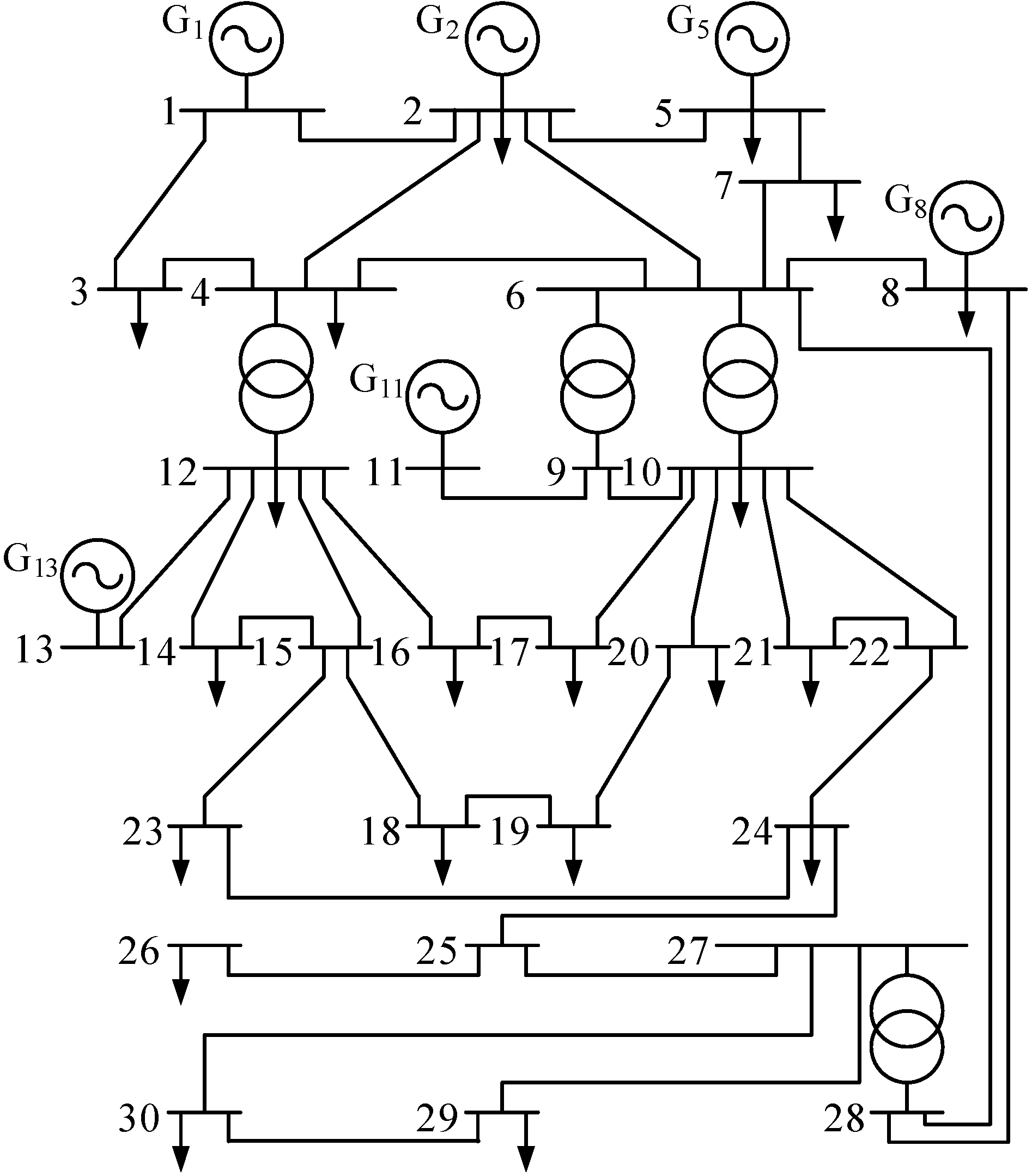
The IEEE 30-bus test system is utilized to test the proposed method. Its total system demand is 283.4 MW for active power and 126.2 MVAR for reactive power. It has six generators, four transformers and nine shunt VAR compensation devices, and has a total of twenty-four control variables for OPF. The limits of the generator buses are 0.95–1.1 p.u., and the transformer-tap settings are assumed to vary in the range [0.9, 1.1] p.u., with step size of 0.0125 p.u. The VAR injections of the shunt capacitors are assumed to vary in the range [0, 5] MVAR, with step size of 1 MVAR. The limits of load buses are 0.95–1.05 p.u., Bus 1 is taken as slack bus. The other control parameters are shown in [12]. The single line diagram of the system is shown in Figure 3.

Figure 3. Single line diagram of the IEEE 30-bus test system.

Figure 3. Single line diagram of the IEEE 30-bus test system.

6.1.1. Convergence Characteristic Analysis

Heuristic optimization algorithms are sensitive to the selection of the control parameters. The IABC algorithm parameters include N_s, L_max, limit, F1, F2 and CR. In order to verify the stability of the proposed IABC algorithm to perturbations of the parameter values, we have simulated different cases with different parameter values in the OPF problem whose optimization objective is the minimization of the fuel cost for the IEEE 30-bus test system. The parameters F1, F2 and CR are introduced in reference [30], and their best values are F1 = F2 = 0.6 and CR = 0.5, respectively.

Case 1: limit = 30 and L_max = 200

In this case, the limit and L_max values are equal to 30 and 200, respectively. The convergence characteristics are analysed for different values of the parameter N_s. Table 1 shows the minimum (Min), average, maximum (Max), and standard deviation (SD) values of fuel cost and average running time obtained by the IABC algorithm with different values of the N_s parameter over 20 independent runs.

Table 1. Results obtained by the IABC algorithm with different N_s values for OPF with total fuel cost.

Ns	Fuel cost ($/h)				Time (s)
	Min	Average	Max	SD
20	800.4320	800.4581	800.5103	0.0240	11.8249
40	800.4296	800.4494	800.4888	0.0159	23.3254
50	800.4259	800.4398	800.4637	0.0096	29.8517
60	800.4244	800.4383	800.4601	0.0090	34.6824
80	800.4228	800.4382	800.4590	0.0082	46.7110
100	800.4215	800.4359	800.4520	0.0081	56.3808
150	800.4212	800.4289	800.4499	0.0070	84.4469
200	800.4194	800.4273	800.4437	0.0066	111.512

Table 1. Results obtained by the IABC algorithm with different N_s values for OPF with total fuel cost.

Ns	Fuel cost ($/h)				Time (s)
	Min	Average	Max	SD
20	800.4320	800.4581	800.5103	0.0240	11.8249
40	800.4296	800.4494	800.4888	0.0159	23.3254
50	800.4259	800.4398	800.4637	0.0096	29.8517
60	800.4244	800.4383	800.4601	0.0090	34.6824
80	800.4228	800.4382	800.4590	0.0082	46.7110
100	800.4215	800.4359	800.4520	0.0081	56.3808
150	800.4212	800.4289	800.4499	0.0070	84.4469
200	800.4194	800.4273	800.4437	0.0066	111.512

From Table 1, it can be seen that the greater the parameter N_s value selected, the smaller the minimum, average and maximum values obtained by the IABC algorithm are, and the longer the running time taken is. The results demonstrate the optimal value changes with different N_s values of the IABC algorithm, and a better objective function value is obtained by the IABC algorithm when a greater N_s value is utilized.

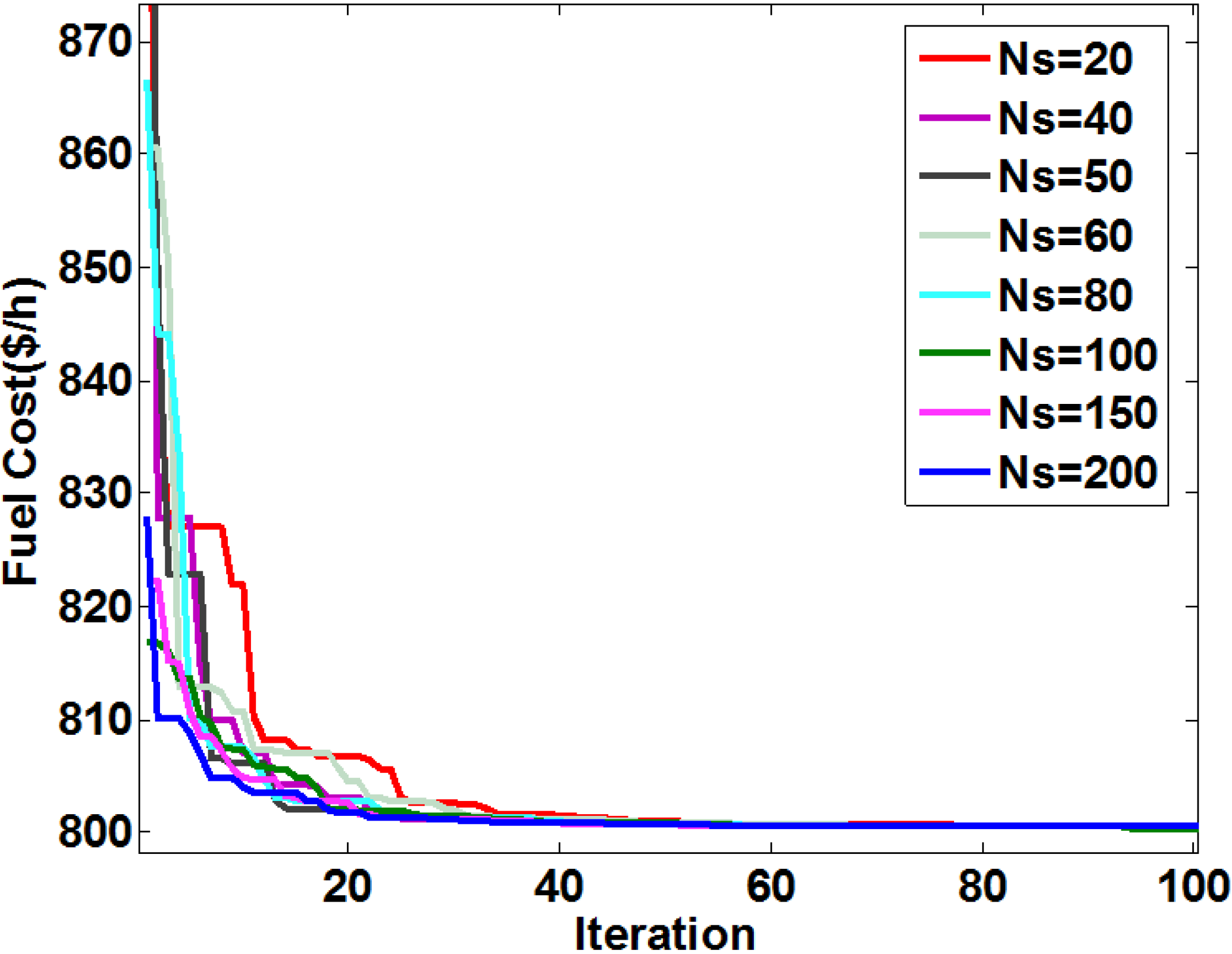
The convergence characteristics of searching for minimum value by IABC algorithm with different parameter N_s values are shown in Figure 4, show which it can be seen that the IABC algorithm is able to converge fast to the corresponding minimum value under the conditions of different parameter settings. The results verify the stability of the IABC algorithm to perturbations of the parameter N_s values.

Figure 4. Convergence characteristics obtained by the IABC algorithms with different values of the parameter N_s for OPF with total fuel cost.

Figure 4. Convergence characteristics obtained by the IABC algorithms with different values of the parameter N_s for OPF with total fuel cost.

Case 2: N_s = 100 and L_max = 200

In this case, the convergence characteristics of the IABC algorithm with different limit parameter values are analyzed. Table 2 shows the minimum, average, maximum, standard deviation values and average running time obtained by the IABC algorithm with different limit parameter values over 20 independent runs.

Table 2. Results obtained by the IABC algorithm with different limit values for OPF with total fuel cost.

Limit	Fuel cost ($/h)				Time (s)
	Min	Average	Max	SD
10	800.4530	800.4818	800.5042	0.0119	56.7482
20	800.4376	800.4561	800.4802	0.0111	58.1910
30	800.4215	800.4359	800.4520	0.0081	56.3808
40	800.4168	800.4291	800.4372	0.0063	56.5577
50	800.4094	800.4200	800.4364	0.0060	56.4471

Table 2. Results obtained by the IABC algorithm with different limit values for OPF with total fuel cost.

Limit	Fuel cost ($/h)				Time (s)
	Min	Average	Max	SD
10	800.4530	800.4818	800.5042	0.0119	56.7482
20	800.4376	800.4561	800.4802	0.0111	58.1910
30	800.4215	800.4359	800.4520	0.0081	56.3808
40	800.4168	800.4291	800.4372	0.0063	56.5577
50	800.4094	800.4200	800.4364	0.0060	56.4471

From Table 2, it can be seen that IABC algorithm with different limit values converges to different optimal values, and the better solution can be obtained with the greater limit parameter value. It also can be seen that the average running time is almost unchanged with the different limit parameter values.

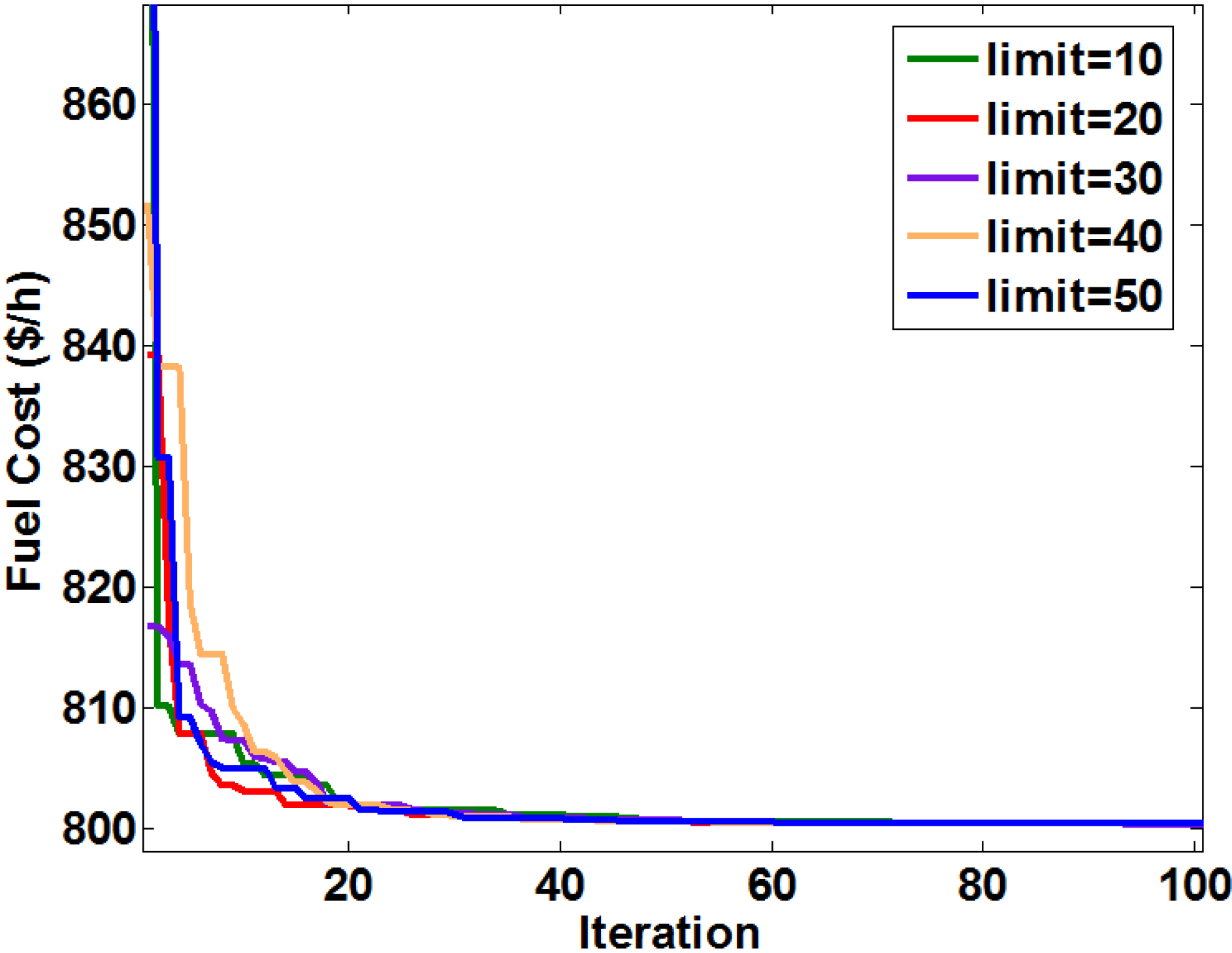
The convergence characteristics of searching for minimum value by IABC algorithm with different limit parameter values are shown in Figure 5, which illustrates that the proposed algorithm with different limit parameter values can quickly and stably converge to the corresponding optimal values. The results demonstrate the stability of the IABC algorithm to perturbations of the limit parameter values.

Figure 5. Convergence characteristics obtained by the IABC algorithm with different parameter limit values for OPF with total fuel cost.

Figure 5. Convergence characteristics obtained by the IABC algorithm with different parameter limit values for OPF with total fuel cost.

Case 3: N_s = 100 and limit = 30

In this case, the purpose of simulation is to analyse the convergence characteristics of the IABC algorithm with different L_max parameter values. The minimum, average, maximum, standard values and average running time obtained by the IABC algorithm with different L_max parameter values after 20 independent runs are tabulated in Table 3.

Table 3. Results obtained by the IABC algorithm with different L_max values for OPF with total fuel cost.

Lmax	Fuel cost ($/h)				Time (s)
	Min	Average	Max	SD
50	800.5383	800.6626	800.8829	0.0860	15.8349
100	800.4284	800.4518	800.4779	0.0137	28.6818
150	800.4249	800.4439	800.4748	0.0121	42.4165
200	800.4215	800.4359	800.4520	0.0081	56.3808
250	800.4192	800.4295	800.4420	0.0080	70.8397
300	800.4177	800.4293	800.4409	0.0072	84.6042

Table 3. Results obtained by the IABC algorithm with different L_max values for OPF with total fuel cost.

Lmax	Fuel cost ($/h)				Time (s)
	Min	Average	Max	SD
50	800.5383	800.6626	800.8829	0.0860	15.8349
100	800.4284	800.4518	800.4779	0.0137	28.6818
150	800.4249	800.4439	800.4748	0.0121	42.4165
200	800.4215	800.4359	800.4520	0.0081	56.3808
250	800.4192	800.4295	800.4420	0.0080	70.8397
300	800.4177	800.4293	800.4409	0.0072	84.6042

As seen from Table 3, the minimum, average, maximum and standard deviation values are better and better with the greater L_max parameter values, and the corresponding running time is longer and longer. The simulation data illustrate the IABC algorithm possesses stability convergence characteristic under the conditions of different L_max parameter values.

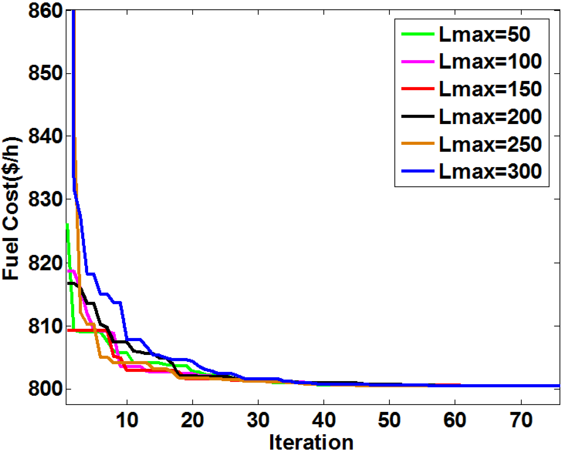
The convergence characteristics of searching for the minimum value by the IABC algorithm with different parameter L_max values are shown in Figure 6, where the proposed IABC algorithm has stable behavior in obtaining the optimal values when different values of the L_max parameter are selected. The simulation verifies the stability of the IABC algorithm to perturbations of the L_max parameter value. Based on the above results of Case 1–Case 3, it can be illustrated that the proposed IABC algorithm possesses stable convergence characteristics and stability to perturbations of the control parameter values.

Figure 6. Convergence characteristics obtained by the IABC algorithm with different L_max parameter values for OPF with total fuel cost.

Figure 6. Convergence characteristics obtained by the IABC algorithm with different L_max parameter values for OPF with total fuel cost.

6.1.2. Single Objective OPF on IEEE 30-Bus Test System

For comprehensive consideration of convergence characteristic and running time, the parameter N_s, limit and L_max values are equal to 100, 30 and 200, respectively. The standard deviation value under these conditions is less than 1% from results of Section 6.1.1, and it illustrates that the IABC algorithm has the better stability.

Firstly, the minimization of total fuel cost described by Equation (3) is selected as objective function for single objective OPF. The results obtained by the proposed IABC approach over 20 independent runs are compared to those obtained by the ABC algorithm, LDI-PSO algorithm [31], GSA algorithm [31], EGA algorithm [32] and IEP algorithm [33]. The results are summarized in the Table 4.

Table 4. Results obtained by different algorithms for OPF with total fuel cost.

Method	Fuel cost ($/h)
	Min	Average	Max
IABC	800.4215	800.4359	800.4520
ABC	800.6850	800.7998	801.1376
LDI-PSO [31]	800.7398	801.5576	803.8698
GSA [31]	805.1752	812.1935	827.4950
EGA [32]	802.0600	–	802.1400
IEP [33]	802.4650	–	–

Table 4. Results obtained by different algorithms for OPF with total fuel cost.

Method	Fuel cost ($/h)
	Min	Average	Max
IABC	800.4215	800.4359	800.4520
ABC	800.6850	800.7998	801.1376
LDI-PSO [31]	800.7398	801.5576	803.8698
GSA [31]	805.1752	812.1935	827.4950
EGA [32]	802.0600	–	802.1400
IEP [33]	802.4650	–	–

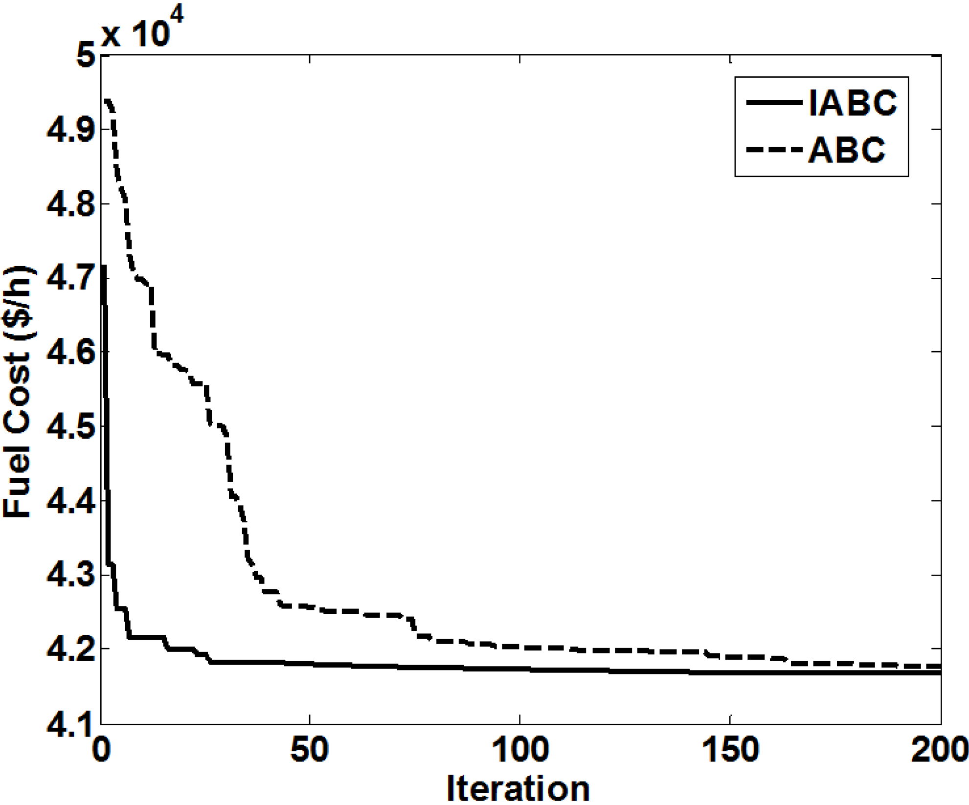
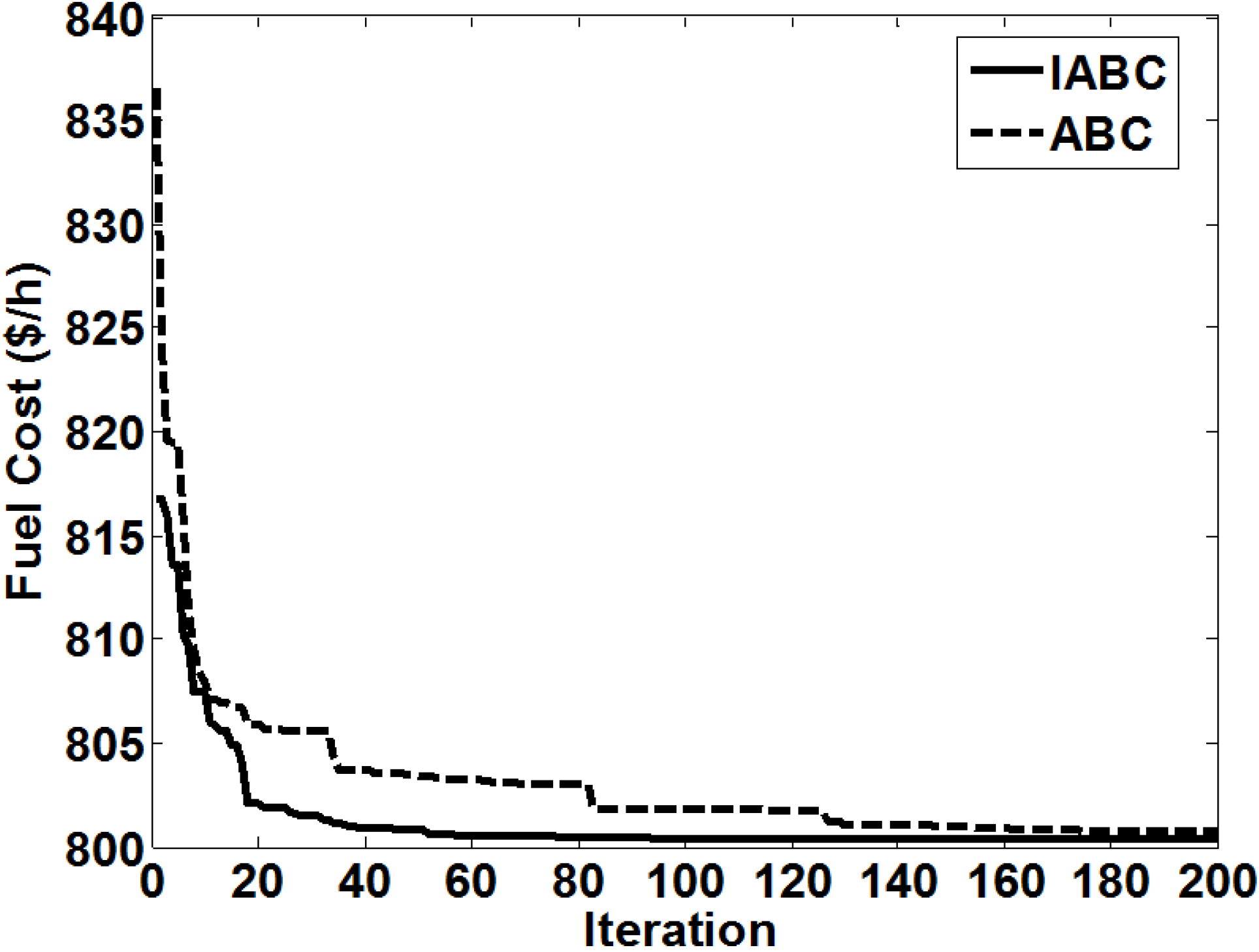
As shown in Table 4, the average total fuel cost value calculated by the IABC algorithm was 800.4359 $/h, and it is obviously less than the other average values calculated by the ABC and other optimization algorithms. The maximum and minimum values calculated by the IABC algorithm are better than those calculated by other algorithms. The results show that the ability of the IABC algorithm to find the optimal solution is better than that of the other algorithms. The convergence characteristics of IABC and ABC algorithms are shown in Figure 7.

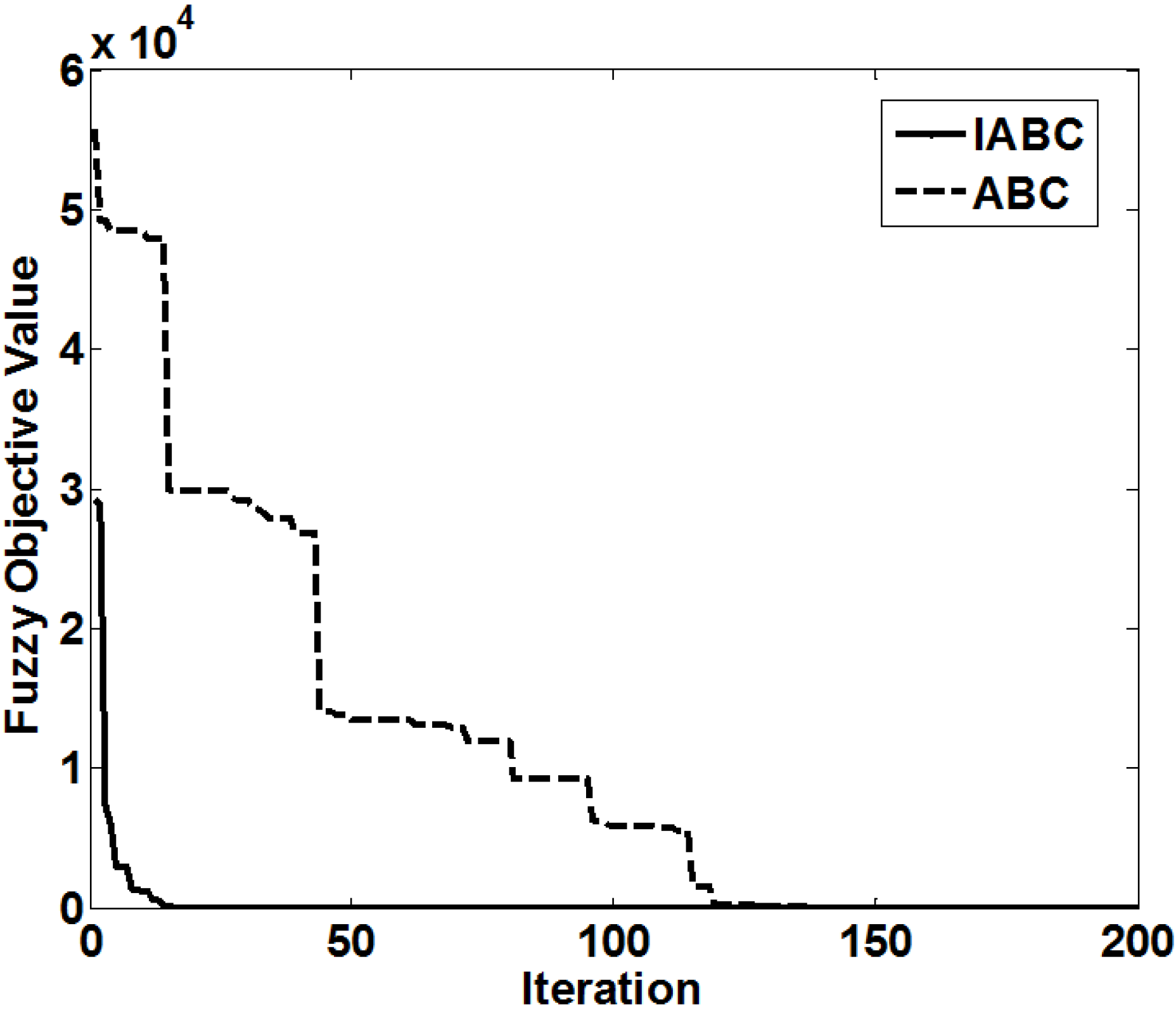
Figure 7. Convergence characteristics of fuel cost for the IABC and ABC algorithms for an IEEE 30-bus system.

Figure 7. Convergence characteristics of fuel cost for the IABC and ABC algorithms for an IEEE 30-bus system.

From Figure 7 and the simulation data, it can be seen that when the iteration number reaches 60, the fuel cost value calculated by IABC is 800.5349 $/h, that is close to global optimal value 800.4215 $/h, however the value calculated by ABC is 804.2461 $/h, that is local optimal value. It also can be seen that the IABC convergence curve is smoother than those of the ABC algorithm. The results demonstrate the convergent performance of the IABC algorithm is better than that of the ABC algorithm.

To further demonstrate the superiority of the IABC algorithm, the other single OPF with different objective functions described by Equations (4)–(6) have been simulated. The results obtained by the IABC algorithm are compared to of the ABC algorithm, MSFLA algorithm [34], GA algorithm [34], PSO algorithm [35], DE algorithm [36], BBO algorithm [37] and DE algorithm [38]. The results are given in the Table 5. 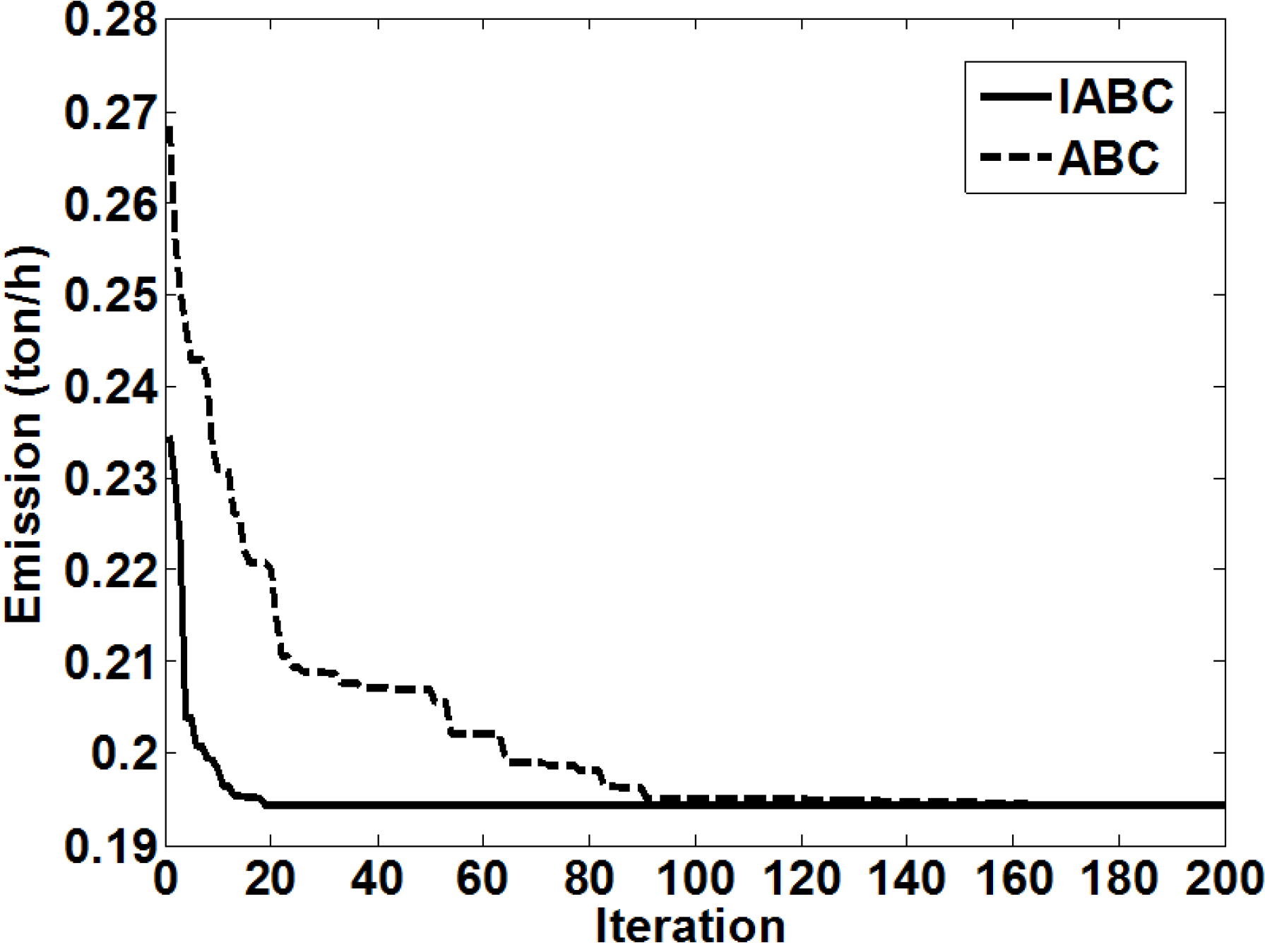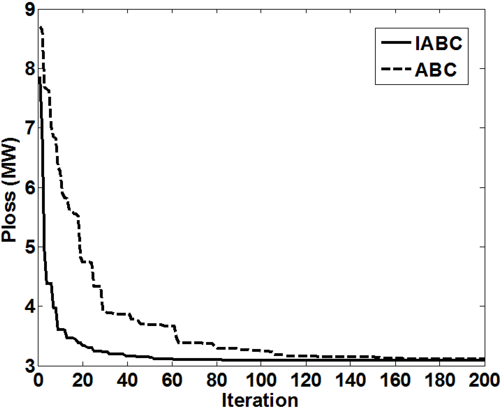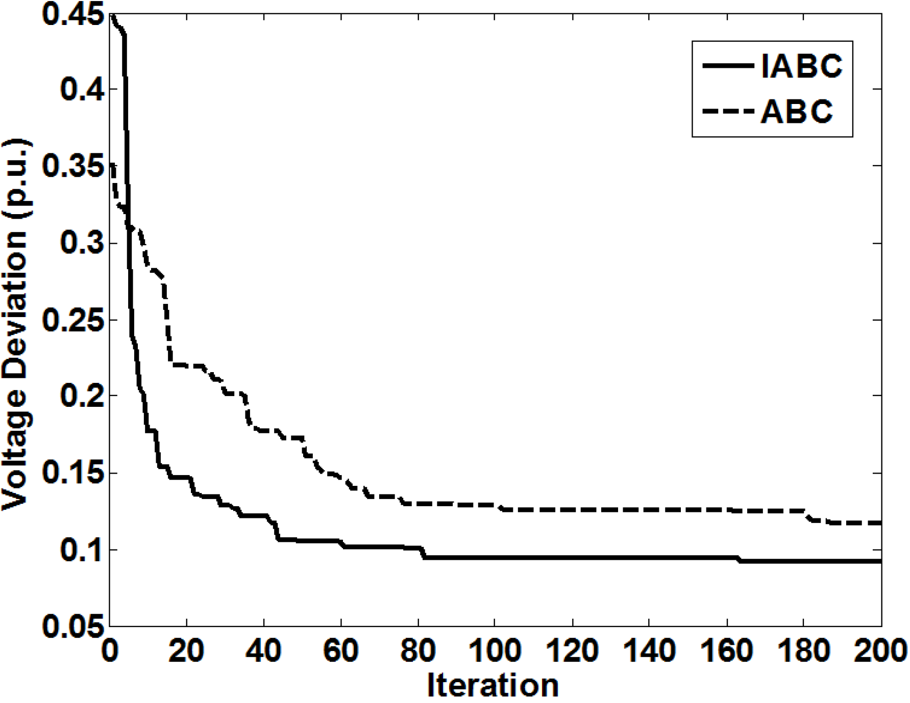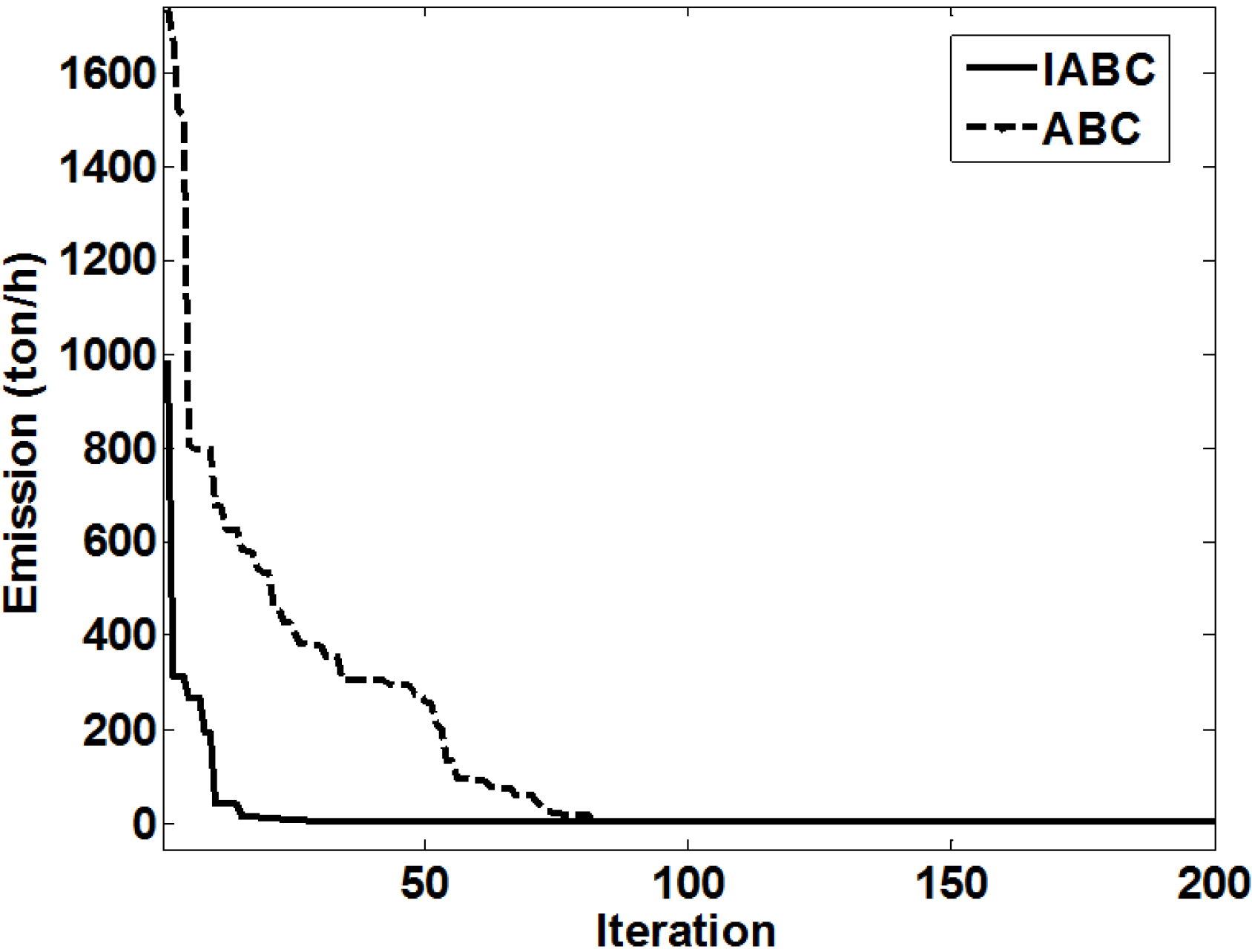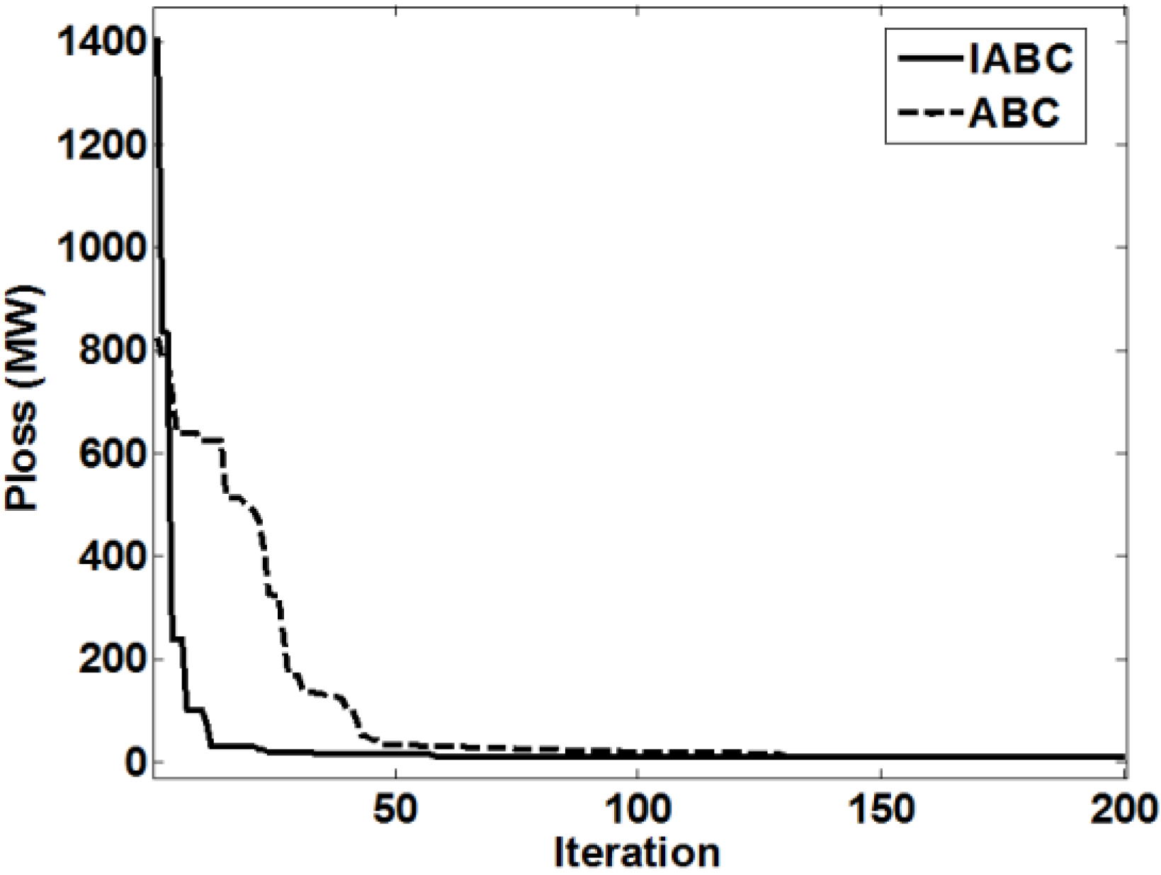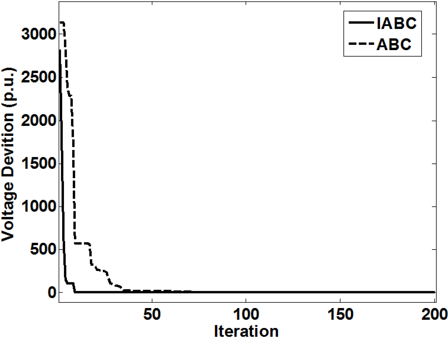As shown in Table 5, the optimal values of total emission, power loss and voltage deviation calculated by IABC are 0.1943 ton/h, 3.0917 MW, 0.0918 p.u., respectively, which are smaller than those calculated by the other algorithms. The results show that the IABC algorithm has better performance than the other algorithms for solving different single objective OPF problems. The convergence characteristics of the IABC and ABC algorithms are shown in Figure 8, Figure 9 and Figure 10.

Table 5. Results obtained by the different algorithms for the single objective OPF.

Method	Objective function
	Emission (ton/h)	Active power loss (MW)	Voltage deviation (p.u.)
IABC	0.1943	3.0917	0.0918
ABC	0.1943	3.1216	0.1179
MSFLA [34]	0.2056	–	–
GA [34]	0.2117	–	–
PSO [35]	–	3.6294	–
DE [36]	–	3.2400	–
BBO [37]	–	–	0.1020
DE [38]	–	–	0.1357

Table 5. Results obtained by the different algorithms for the single objective OPF.

Method	Objective function
	Emission (ton/h)	Active power loss (MW)	Voltage deviation (p.u.)
IABC	0.1943	3.0917	0.0918
ABC	0.1943	3.1216	0.1179
MSFLA [34]	0.2056	–	–
GA [34]	0.2117	–	–
PSO [35]	–	3.6294	–
DE [36]	–	3.2400	–
BBO [37]	–	–	0.1020
DE [38]	–	–	0.1357

Figure 8. Convergence characteristics of total emission of the IABC and ABC algorithms for the IEEE 30-bus system.

Figure 8. Convergence characteristics of total emission of the IABC and ABC algorithms for the IEEE 30-bus system.

From Figure 8 and simulation data, it can be seen that when the iteration number reaches up to 20 the emission value of 0.1943 ton/h calculated by the IABC algorithm is a global optimal value, however the value calculated by the ABC algorithm is a local optimal value. From Figure 9 and Figure 10, it also can be seen that the IABC algorithm converges to highest quality solution among the other algorithms in less iterations. In additional, it can be seen that the convergence curve of the IABC one is smoother than that of the other algorithms. The results demonstrate that the convergence rate and convergence capacity of the IABC algorithm are obviously better than those of the ABC algorithm.

From the results of Section 6.1.2, it can be seen that the convergence capacity and the optimal value of the IABC algorithm are better than those of the ABC algorithm and other heuristic algorithms, which demonstrates the effectiveness and superiority of the IABC algorithm to solve the single objective OPF problem.

Figure 9. Convergence characteristics of power loss of the IABC and ABC algorithms for the IEEE 30-bus system.

Figure 9. Convergence characteristics of power loss of the IABC and ABC algorithms for the IEEE 30-bus system.

Figure 10. Convergence characteristics of voltage deviation of the IABC and ABC algorithms for the IEEE 30-bus system.

Figure 10. Convergence characteristics of voltage deviation of the IABC and ABC algorithms for the IEEE 30-bus system.

6.1.3. Fuzzy Multi-Objective OPF on IEEE 30-Bus Test System

The results calculated in Section 6.1.2 are utilized as the reference values of the fuzzy membership function. Four objective functions are converted into fuzzy multi-objective ones by Equations (16) and (17), and the proposed method is used to solve the fuzzy multi-objective OPF problem. The optimal values calculated by the IABC and ABC algorithms for multi-objective OPF are given in Table 6.

As shown in Table 6, the fuzzy fitness value calculated by the IABC algorithm is 0.7685, which is better than the 0.7571 value calculated by the ABC algorithm, and each objective function value obtained by the IABC algorithm is smaller than those provided by the ABC algorithm. The results indicate that the optimal scheme obtained by the proposed model can make systems more economical and stable than those possible with the ABC algorithm. The convergence characteristics of the IABC and ABC algorithm for multi-objective OPF are shown in Figure 11.

Table 6. Results obtained by the different algorithms for fuzzy multi-objective OPF.

Optimization method	Objective function
	Fuel cost ($/h)	Emission (ton/h)	Active power loss (MW)	Voltage deviation (p.u)	Fitness value
IABC	851.6111	0.2230	4.8731	0.3044	0.7685
ABC	854.9166	0.2280	4.9820	0.3590	0.7571

Table 6. Results obtained by the different algorithms for fuzzy multi-objective OPF.

Optimization method	Objective function
	Fuel cost ($/h)	Emission (ton/h)	Active power loss (MW)	Voltage deviation (p.u)	Fitness value
IABC	851.6111	0.2230	4.8731	0.3044	0.7685
ABC	854.9166	0.2280	4.9820	0.3590	0.7571

Figure 11. Multi-objective convergence characteristic curves of the IABC and ABC algorithms for the IEEE 30-bus system.

Figure 11. Multi-objective convergence characteristic curves of the IABC and ABC algorithms for the IEEE 30-bus system.

From Figure 11, it can be seen that the fuzzy optimal value obtained by the IABC algorithm is smaller than that given by the ABC algorithm. In addition, the convergence characteristic curve of the IABC algorithm is smoother than that of the ABC algorithm. The results illustrate that the convergence capacity of the IABC algorithm is better than that of the ABC algorithm.

6.2. IEEE 57-Bus Test System

To further verify the performance of the proposed IABC algorithm, the IEEE 57-bus system was also used as a test system. The IEEE 57-bus test system consists of 80 transmission lines, seven generators, 15 branches under load tap setting transformer branches and three shunt reactive power sources at the buses 18, 25 and 53. The total load demand of the test system is 1250.8 MW and 336.4 MVAR. The bus data, line data, generator data, cost and emission coefficients are taken from references [39]. The proposed IABC algorithm is utilized to solve single objective OPF and multi-objective OPF on the IEEE 57-bus system.

6.2.1. Single Objective OPF on the IEEE 57-Bus Test System

The four objective functions are considered as the optimization objective of OPF on the IEEE 57-bus system, respectively. The simulation results obtained by the IABC algorithm and standard ABC algorithm over 20 independent runs are tabulated in Table 7.

Table 7. Results obtained by the IABC and ABC algorithms for different single objective OPF for the IEEE 57-bus system.

Compared item	Optimization objective function
	Fuel cost ($/h)		Emission (ton/h)		Active power loss (MW)		Voltage deviation (p.u)
	IABC	ABC	IABC	ABC	IABC	ABC	IABC	ABC
Min	41684	41781	1.0484	1.2048	11.1574	12.6260	0.6616	0.8514
Average	41698	41840	1.1382	1.3262	11.9855	13.7754	0.7693	0.9376
Max	41711	41927	1.3709	1.6351	13.7499	15.6453	0.8992	1.1081
SD	7.7840	38.2438	0.0789	0.1202	0.7140	0.7917	0.0538	0.0719
Time (s)	94.7014	95.7394	96.2508	96.5339	93.9822	98.2990	94.9440	98.7224

Table 7. Results obtained by the IABC and ABC algorithms for different single objective OPF for the IEEE 57-bus system.

Compared item	Optimization objective function
	Fuel cost ($/h)		Emission (ton/h)		Active power loss (MW)		Voltage deviation (p.u)
	IABC	ABC	IABC	ABC	IABC	ABC	IABC	ABC
Min	41684	41781	1.0484	1.2048	11.1574	12.6260	0.6616	0.8514
Average	41698	41840	1.1382	1.3262	11.9855	13.7754	0.7693	0.9376
Max	41711	41927	1.3709	1.6351	13.7499	15.6453	0.8992	1.1081
SD	7.7840	38.2438	0.0789	0.1202	0.7140	0.7917	0.0538	0.0719
Time (s)	94.7014	95.7394	96.2508	96.5339	93.9822	98.2990	94.9440	98.7224

As shown in Table 7, all the minimum, average, maximum and standard deviation values obtained by the IABC algorithm are better than those obtained by the ABC algorithm for solving the OPF problem with different optimization objectives. Moreover, the results in Table 7 also show that the average computation time of the 20 independent runs for proposed algorithm is shorter than the time for the ABC algorithm under the different optimization objective conditions. The results illustrate that the effectiveness and superiority of the proposed IABC algorithm for solving the OPF problem, and that it can converge to a better solution compared with the ABC algorithm. The convergence characteristics of the IABC and ABC algorithms for single objective OPF with different objective functions on the IEEE 57-bus system are shown in Figure 12, Figure 13, Figure 14 and Figure 15, respectively.

From Figure 12, Figure 13, Figure 14 and Figure 15, it can be seen that the proposed IABC algorithm converges to better solutions much faster than the standard ABC algorithm. The results illustrate that the proposed method possesses better convergence characteristics for solving OPF problems.

Figure 12. Convergence characteristics of fuel cost of the IABC and ABC algorithms for the IEEE 57-bus system.

Figure 12. Convergence characteristics of fuel cost of the IABC and ABC algorithms for the IEEE 57-bus system.

Figure 13. Convergence characteristics of emissions of the IABC and ABC algorithm for the IEEE 57-bus system.

Figure 13. Convergence characteristics of emissions of the IABC and ABC algorithm for the IEEE 57-bus system.

Figure 14. Convergence characteristics of power loss of the IABC and ABC algorithms for the IEEE 57-bus system.

Figure 14. Convergence characteristics of power loss of the IABC and ABC algorithms for the IEEE 57-bus system.

Figure 15. Convergence characteristics of voltage deviation of the IABC and ABC algorithms for the IEEE 57-bus system.

Figure 15. Convergence characteristics of voltage deviation of the IABC and ABC algorithms for the IEEE 57-bus system.

6.2.2. Fuzzy Multi-Objective OPF on the IEEE 57-Bus Test System

In this case, the proposed IABC algorithm is used to solve the fuzzy multi-objective OPF problem for the IEEE 57-bus system. The minimum, average, maximum fitness values and standard deviation value calculated by the IABC and ABC algorithms over 20 independent runs are given in Table 8. The best objective values obtained by the IABC and ABC algorithms over 20 independent runs are shown in Table 9.

Table 8. Results obtained by the different algorithms for fuzzy multi-objective OPF for the IEEE 57-bus system.

Optimization method	Fuzzy fitness value				Average time (s)
	Max	Average	Min	SD
IABC	0.7393	0.6697	0.5652	0.0367	90.8029
ABC	0.6910	0.6103	0.5072	0.0560	91.2489

Table 8. Results obtained by the different algorithms for fuzzy multi-objective OPF for the IEEE 57-bus system.

Optimization method	Fuzzy fitness value				Average time (s)
	Max	Average	Min	SD
IABC	0.7393	0.6697	0.5652	0.0367	90.8029
ABC	0.6910	0.6103	0.5072	0.0560	91.2489

Table 9. Best solutions obtained by the different algorithms for fuzzy multi-objective OPF for the IEEE 57-bus system.

Optimization method	Objective value				Fitness value
	Fuel Cost ($/h)	Emissions (ton/h)	Active power loss (MW)	Voltage deviation (p.u.)
IABC	44,152	1.2643	16.6196	0.9642	0.7393
ABC	44,741	1.3396	17.6643	0.9728	0.6910

Table 9. Best solutions obtained by the different algorithms for fuzzy multi-objective OPF for the IEEE 57-bus system.

Optimization method	Objective value				Fitness value
	Fuel Cost ($/h)	Emissions (ton/h)	Active power loss (MW)	Voltage deviation (p.u.)
IABC	44,152	1.2643	16.6196	0.9642	0.7393
ABC	44,741	1.3396	17.6643	0.9728	0.6910

As seen from Table 8, the maximum, average and minimum values obtained by the IABC algorithm are greater than those given by the ABC algorithm, and the standard deviation value calculated by the proposed approach is less than that provided by the ABC algorithm. Moreover, the average running time of the IABC algorithm is shorter than that of the ABC algorithm. The results demonstrate that the IABC algorithm can obtain better solutions compared with the standard ABC algorithm in less running time.

By comparing the fuel cost, emissions, active power loss and voltage deviation results from the IABC algorithm and ABC algorithm (Table 9), it can be seen that the values of all the objectives obtained by the IABC algorithm are less than those given by the ABC algorithm. The results illustrate the superiority of the proposed IABC algorithm for solving the multi-objective OPF. The convergence characteristics of the IABC and ABC algorithm for multi-objective OPF for the IEEE 57-bus system are shown in Figure 16.

Figure 16. Convergence characteristics of the IABC and ABC algorithms for multi-objective OPF for the IEEE 57-bus system.

Figure 16. Convergence characteristics of the IABC and ABC algorithms for multi-objective OPF for the IEEE 57-bus system.

Figure 16 illustrates that the proposed IABC algorithm can converge to higher quality solutions compared with the ABC algorithm in less iterations. The results verify the IABC algorithm possesses better convergence characteristics compared with the ABC algorithm.

6.3. IEEE 300-Bus Test System

In order to demonstrate the effectiveness of the proposed IABC algorithm, the IEEE 300-bus system was also used as a test system. The network includes 69 generators, 107 transformers and 29 shunt reactive power sources. The system data are taken from reference [40]. The simulation results obtained by the IABC algorithm and standard ABC algorithm over 10 independent runs for single objective OPF are tabulated in Table 10.

Table 10. Results obtained by the IABC and ABC algorithms for different single objective OPF for the IEEE 300-bus system.

Compared item	Optimization objective function
	Fuel cost ($/h)		Emission (ton/h)		Active power loss (MW)		Voltage deviation (p.u)
	IABC	ABC	IABC	ABC	IABC	ABC	IABC	ABC
Min	783951	785474	6.1895	6.1943	295.4514	313.2970	5.5178	5.7047
Average	783956	785861	6.1938	6.2029	295.5136	319.1695	5.5826	5.8782
Max	783965	786159	6.2018	6.2102	295.5813	327.1119	5.6232	6.0778
SD	5.8992	296.8968	0.0051	0.0056	0.0347	4.9314	0.0426	0.1323
Time (s)	582.7570	597.3479	582.7750	596.1126	577.4225	580.8112	576.9575	582.3205

Table 10. Results obtained by the IABC and ABC algorithms for different single objective OPF for the IEEE 300-bus system.

Compared item	Optimization objective function
	Fuel cost ($/h)		Emission (ton/h)		Active power loss (MW)		Voltage deviation (p.u)
	IABC	ABC	IABC	ABC	IABC	ABC	IABC	ABC
Min	783951	785474	6.1895	6.1943	295.4514	313.2970	5.5178	5.7047
Average	783956	785861	6.1938	6.2029	295.5136	319.1695	5.5826	5.8782
Max	783965	786159	6.2018	6.2102	295.5813	327.1119	5.6232	6.0778
SD	5.8992	296.8968	0.0051	0.0056	0.0347	4.9314	0.0426	0.1323
Time (s)	582.7570	597.3479	582.7750	596.1126	577.4225	580.8112	576.9575	582.3205

It is observed from the results in Table 10 that the minimum, average, maximum and standard deviation values of each optimization objective from IABC algorithm are better than ABC algorithm. Moreover, the computation time of proposed method is shorter than the time of ABC algorithm. The proposed IABC algorithm is also used to solve the fuzzy multi-objective OPF problem for the IEEE 300-bus system. The minimum, average, maximum fitness values and standard deviation value calculated by the IABC and ABC algorithms over 10 independent runs are given in Table 11. The best objective values obtained by the IABC and ABC algorithms over 10 independent runs are shown in Table 12.

From Table 11 and Table 12, it can be seen that the each objective value and fuzzy fitness value obtained by the IABC algorithm are better than those given by the ABC algorithm. The results illustrate the superiority of the proposed IABC algorithm for solving the multi-objective OPF. The convergence characteristics of the IABC and ABC algorithm for multi-objective OPF for the IEEE 300-bus system are shown in Figure 17.

Table 11. Results obtained by the different algorithms for fuzzy multi-objective OPF for the IEEE 300-bus system.

Optimization method	Fuzzy fitness value				Average time (s)
	Max	Average	Min	SD
IABC	0.9183	0.9127	0.9045	0.0055	580.6995
ABC	0.8203	0.7870	0.7477	0.0326	587.2060

Table 11. Results obtained by the different algorithms for fuzzy multi-objective OPF for the IEEE 300-bus system.

Optimization method	Fuzzy fitness value				Average time (s)
	Max	Average	Min	SD
IABC	0.9183	0.9127	0.9045	0.0055	580.6995
ABC	0.8203	0.7870	0.7477	0.0326	587.2060

Table 12. Best solutions obtained by the different algorithms for fuzzy multi-objective OPF for the IEEE 300-bus system.

Optimization method	Objective value				Fitness value
	Fuel cost ($/h)	Emissions (ton/h)	Active power loss (MW)	Voltage deviation (p.u.)
IABC	785360	6.1934	297.6362	5.9169	0.9183
ABC	788657	6.1995	321.2646	5.9608	0.8203

Table 12. Best solutions obtained by the different algorithms for fuzzy multi-objective OPF for the IEEE 300-bus system.

Optimization method	Objective value				Fitness value
	Fuel cost ($/h)	Emissions (ton/h)	Active power loss (MW)	Voltage deviation (p.u.)
IABC	785360	6.1934	297.6362	5.9169	0.9183
ABC	788657	6.1995	321.2646	5.9608	0.8203

Figure 17. Convergence characteristics of the IABC and ABC algorithms for multi-objective OPF for the IEEE 300-bus system.

Figure 17. Convergence characteristics of the IABC and ABC algorithms for multi-objective OPF for the IEEE 300-bus system.

Figure 17 illustrates that the proposed IABC algorithm can converge to a better solution much faster than ABC algorithm. The results demonstrate the effectiveness and superiority of proposed method for solving OPF problem to larger scale system.

7. Conclusions

In this paper, we have presented an improved artificial bee colony (IABC) algorithm based on mutation operation, crossover operation and tent chaos mapping. The IABC algorithm is applied to solve the OPF problem with four different objective functions which are considered to minimize the fuel cost, emissions, power losses and voltage deviation. The proposed approach is successfully implemented on the IEEE 30-bus, IEEE 57-bus and IEEE 300-bus test systems. The simulation indicates the proposed approach possesses better convergence characteristics, and furthermore, the results illustrate that the IABC algorithm is efficient and superior at solving OPF problems, and the obtained optimal scheme can make power systems more economical and stable.