
Optimal Dispatch Strategy of a Virtual Power Plant Containing Battery Switch Stations in a Unified Electricity Market

Abstract
:
1. Introduction

2. Trading Model in a Unified Electricity Market
2.1. Power Purchases in a Unified Market
2.2. Power Selling in a Unified Market
3. Optimal Dispatch Strategy
3.1. Objective Function
3.2. Grid Security and Power Balance Constraints
3.3. DG Model
3.3.1. Operation Constraints
3.3.2. Operation Costs
3.4. IL Model
3.4.1. Operation Benefits and Costs
3.4.2. Operation Constraints
3.5. ESS Model
3.5.1. Operation Costs
3.5.2. Operation Constraints
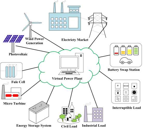
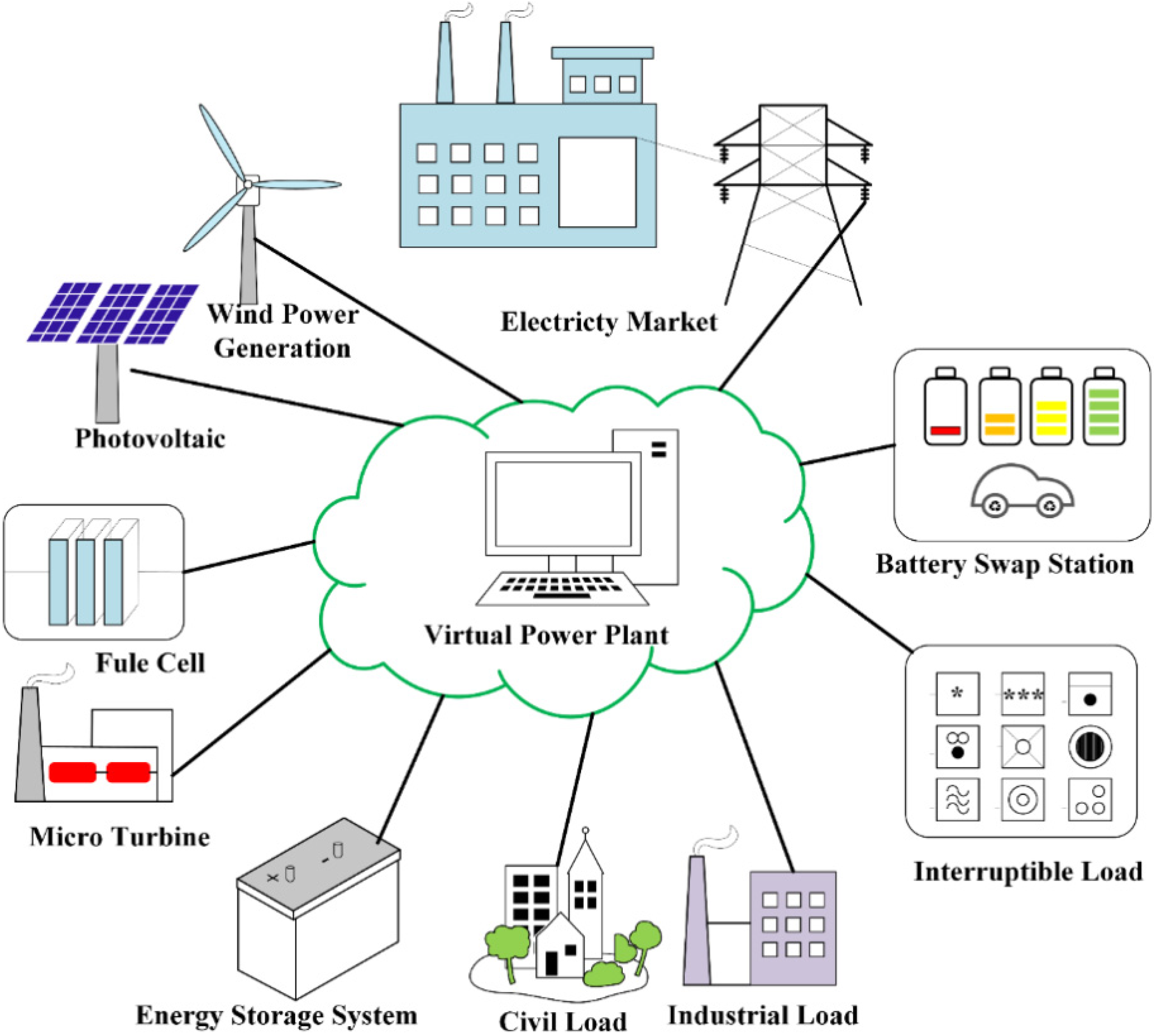
3.6. BSS Model
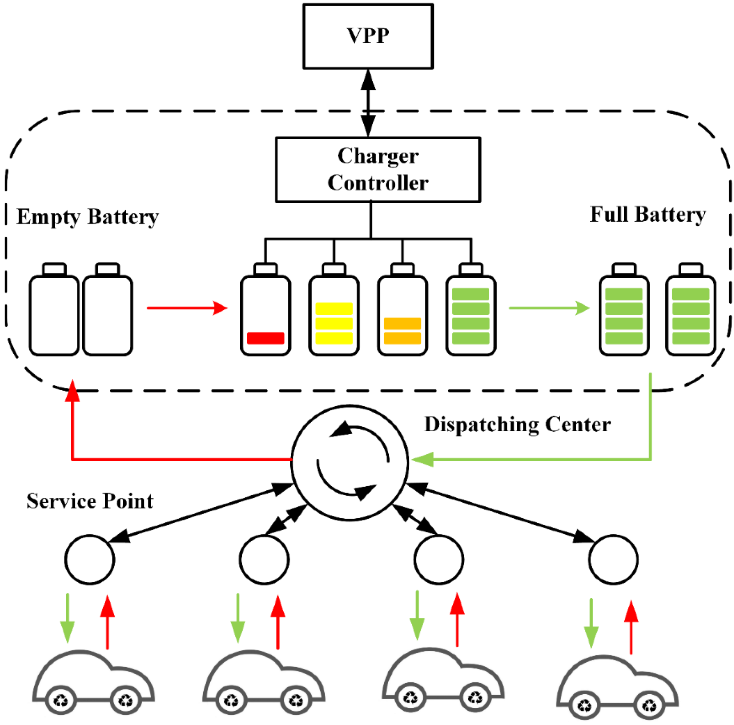
3.6.1. Operation Benefits
- (1)
- Service points charge a battery rental fee from EV consumers, after deducting the battery depreciation cost caused by charge, so the BSS’s net benefits can be expressed as:where α is the battery rental fee for one battery pack; β is the battery depreciation cost for one discharge; rc is the replacement cost for one battery pack; is the cycle life of battery pack i at time t; is the demand of battery packs at the service points in unit time; is the mean power purchase price during the charging of battery pack ; is the charging efficiency of the battery pack; is the rated capacity of the battery pack; is the battery demand of EVs; is the number of full charged battery packs in charger i at time t.
- (2)
- BSS earn profits by selling power to the grid at a high price and purchasing power from the grid at a lower price:where is the number of charge-discharge cycles for a battery pack selling power to the grid in unit time; is the aging cost coefficient; is the total depreciation cost of a battery selling power to the grid in unit time; and are the mean power purchase price and mean power selling price for a battery pack ; is the discharging efficiency of the battery pack; is the power sold to the grid by discharging the battery pack ; is the SOC of battery pack i at time t.
3.6.2. Operation Constraints
- (1)
- Charger controller constraint:where is a binary variable denoting the charge decision for charger i at time t; is a binary variable denoting the discharge decision for charger i at time t:where and are the charge power and discharge power for charger i at time t; and are the maximum and minimum charge power for charger i; and are the maximum and minimum discharge power for charger i.where and are the ramp-down and ramp-up limits of the charge power for charger i; and are the ramp-down and ramp-up limits of the discharge power for charger i; is unit time.
- (2)
- State flag constraint:where is a flag denoting the state of charger i at time t changing to charge from discharge; is a flag denoting the state of charger i at time t changing to discharge from charge:where is a flag denoting the charger i complete charging at time t; is a flag denoting the charger i completing discharge at time t.To expand the battery service life, the online battery must complete charging before its state changes to discharge from charge, and besides the online battery must complete discharge before its state changes to charge from discharge:
- (3)
- SOC constraint:where is the power charged by charger i at time t.
4. Fruit Fly Optimization Algorithm
- (1)
- Initialize the fruit fly swarm location , and set the maximum number of generations and population size;
- (2)
- Give the random direction and distance for foraging using osphresis by an individual fruit fly:where is the fixed step size of a fruit fly using osphresis for foraging.
- (3)
- Calculate the smell concentration judgment value for each fruit:where is the distance of the food location to the origin;
- (4)
- Calculate the smell concentration for each fruit by substituting into the smell concentration judgment function, then find the fruit fly with maximal smell concentration:
- (5)
- Record the maximal smell concentration value and x, y coordinates. Then, the fruit flies swarm towards that location with the maximal smell concentration value by using vision:
- (6)
- End the algorithm if the maximum number of generations is reached; otherwise, repeat the implementation of steps (2)–(3).
5. Study Case
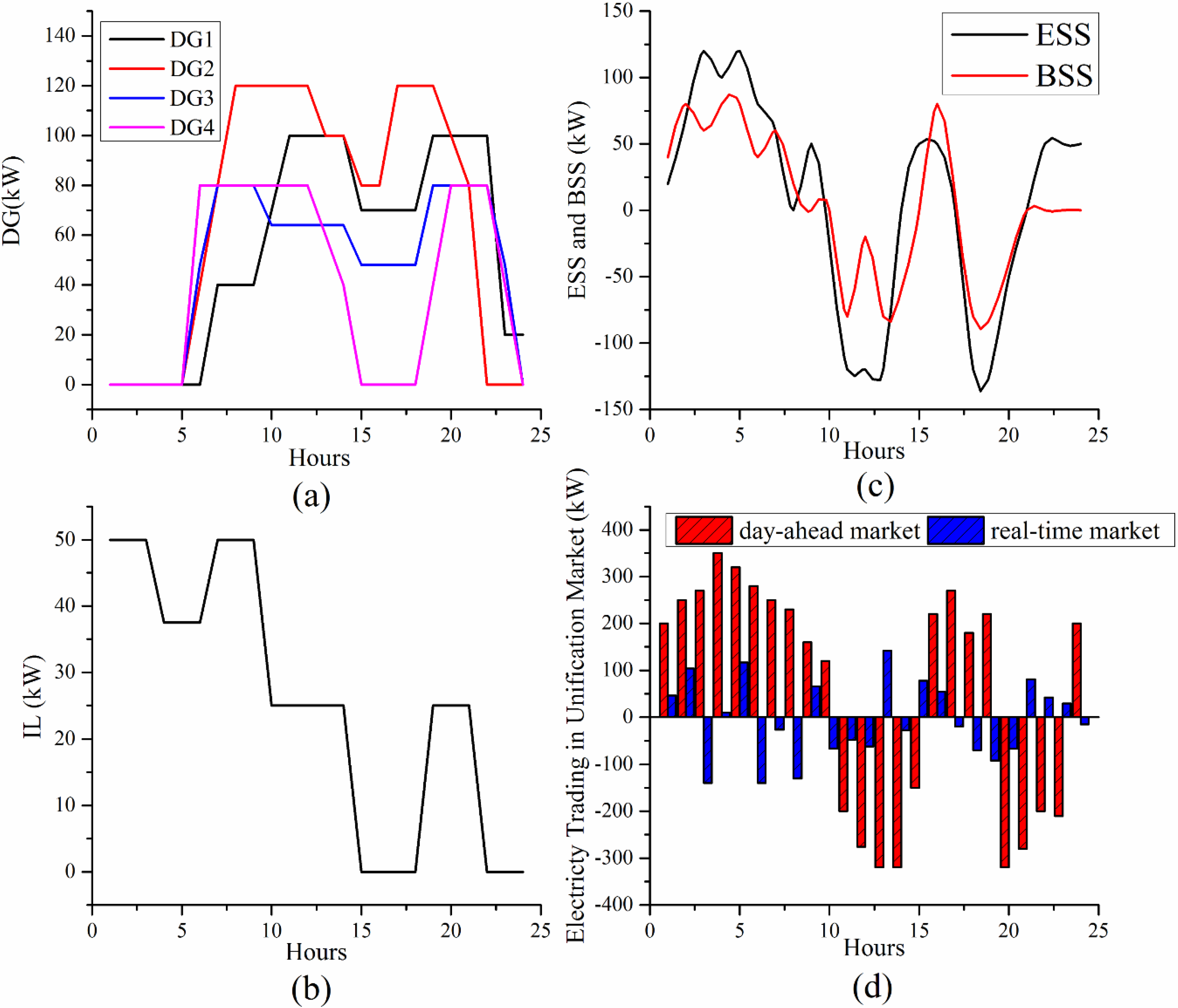
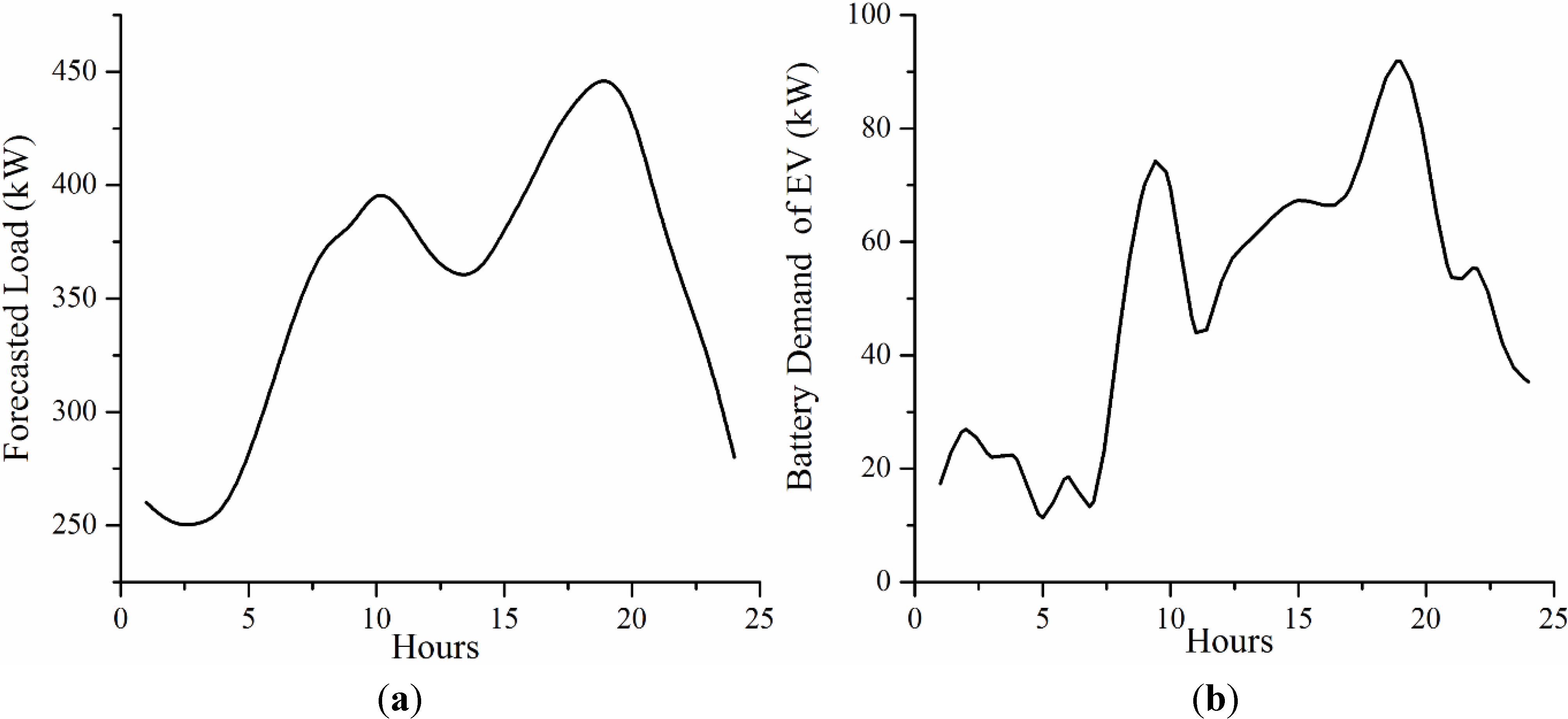
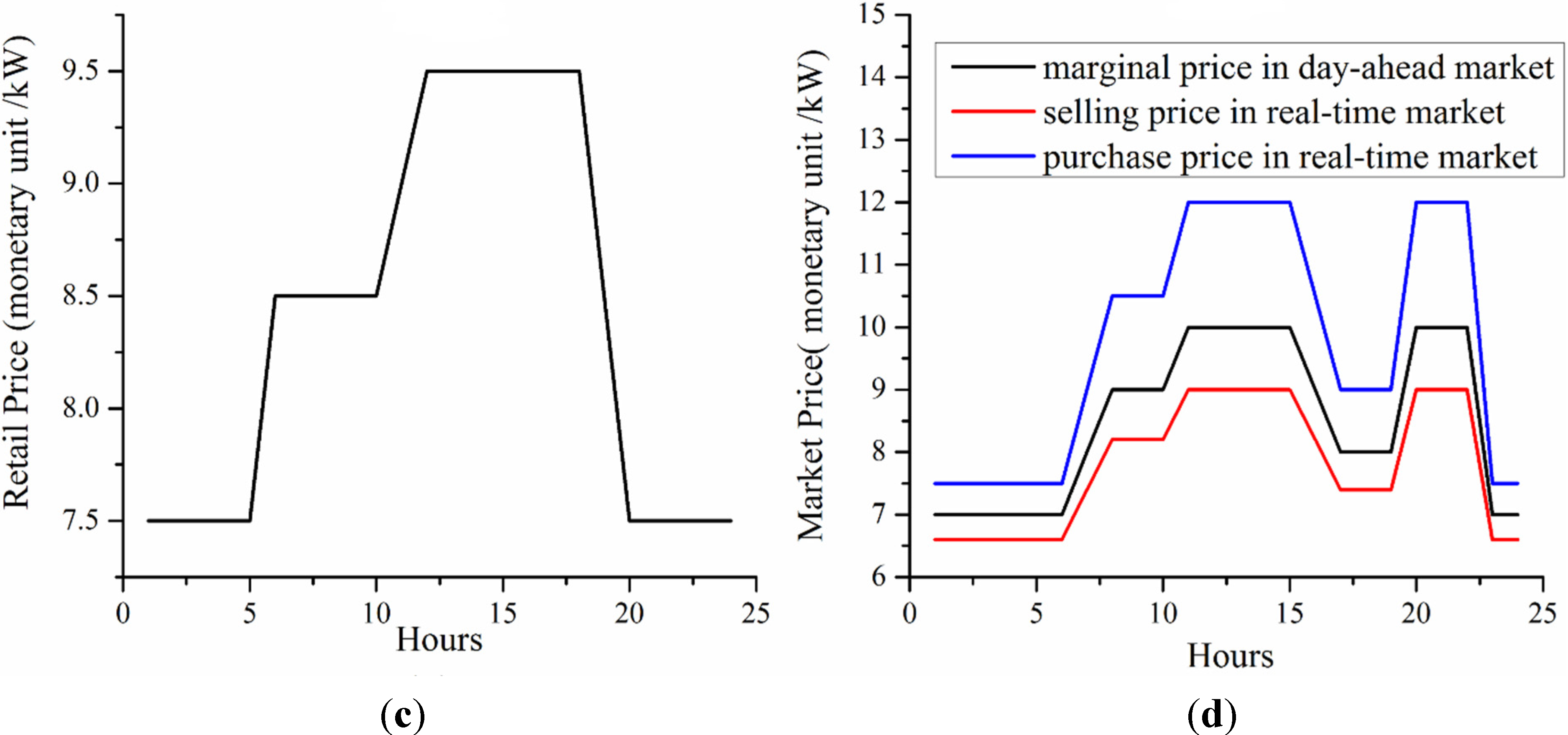
5.1. Test System


| DG | Pmin | Pmax | a | b | MUT | MDT | RUP | RDN | SUC | SDC |
|---|---|---|---|---|---|---|---|---|---|---|
| DG1 | 0 | 100 | 0.01 | 10.5 | 2 | 2 | 10 | 10 | 8.5 | 8.5 |
| DG2 | 0 | 120 | 0.01 | 8.5 | 1.5 | 1.5 | 12.5 | 12.5 | 10.3 | 10.3 |
| DG3 | 0 | 80 | 0.01 | 9.2 | 1 | 1 | 17.5 | 17.5 | 7.6 | 7.6 |
| DG4 | 0 | 80 | 0.01 | 12.6 | 4 | 4 | 14 | 14 | 15 | 15 |
| t | 1 | 2 | 3 | 4 | 5 | 6 | 7 | 8 | 9 | 10 | 11 | 12 |
|---|---|---|---|---|---|---|---|---|---|---|---|---|
| δ(t) | 13 | 12 | 11.5 | 12.5 | 14 | 15.5 | 17 | 19 | 18.5 | 20 | 19.5 | 18.5 |
| t | 13 | 14 | 15 | 16 | 17 | 18 | 19 | 20 | 21 | 22 | 23 | 24 |
| δ(t) | 18 | 18 | 19 | 20 | 21 | 22 | 22.5 | 22 | 19.5 | 17 | 16 | 14 |
5.2. Simulation Result and Discussion

| Hour | Revenue in Unified Market | Cost in Unified Market | Net Benefits in Unified Market | Net Benefits in Separate Market |
|---|---|---|---|---|
| 1 | 941.7 | 623.1 | 318.6 | 181.6 |
| 2 | 729.9 | 507.7 | 222.2 | 165.2 |
| 3 | 801.9 | 566.0 | 235.9 | 165.9 |
| 4 | 863.3 | 649.9 | 213.4 | 163.4 |
| 5 | 1,008.3 | 707.4 | 300.8 | 180.8 |
| 6 | 1,390.2 | 1,005.1 | 385.1 | 320.1 |
| 7 | 1,476.4 | 1,005.1 | 471.3 | 341.3 |
| 8 | 1,751.3 | 1,230.3 | 521.0 | 386.0 |
| 9 | 1,931.9 | 1,313.3 | 618.6 | 492.6 |
| 10 | 1,954.4 | 1,313.3 | 641.2 | 518.2 |
| 11 | 1,517.4 | 1,042.9 | 474.5 | 328.5 |
| 12 | 2,055.9 | 1,313.3 | 742.6 | 626.6 |
| 13 | 2,063.2 | 1,218.5 | 844.7 | 753.7 |
| 14 | 1,848.8 | 1,218.5 | 630.3 | 530.3 |
| 15 | 1,481.4 | 999.7 | 481.8 | 418.8 |
| 16 | 1,085.0 | 707.4 | 377.5 | 234.5 |
| 17 | 1,376.1 | 1,064.6 | 311.5 | 238.5 |
| 18 | 1,356.2 | 1,064.6 | 291.6 | 213.6 |
| 19 | 1,915.7 | 1,360.7 | 555.0 | 472.0 |
| 20 | 2,088.9 | 1,360.1 | 728.8 | 597.8 |
| 21 | 2,359.0 | 1,467.3 | 891.7 | 755.7 |
| 22 | 1,993.9 | 1,467.3 | 526.6 | 447.6 |
| 23 | 1,046.6 | 707.4 | 339.2 | 249.2 |
| 24 | 1,473.2 | 1,113.3 | 359.9 | 309.9 |
| Total | 36,510.6 | 25,026.8 | 11,483.8 | 9,091.8 |
6. Conclusions
Acknowledgments
Author Contributions
Conflicts of Interest
References
- El-Khattam, W.; Salama, M.M.A. Distributed generation technologies, definitions and benefits. Electr. Power Syst. Res. 2004, 71, 119–128. [Google Scholar] [CrossRef]
- Pudjianto, D.; Ramsay, C.; Strbac, G. Virtual power plant and system integration of distributed energy resources. IET Renew. Power Gener. 2007, 1, 10–16. [Google Scholar] [CrossRef]
- Mashhour, E.; Moghaddas-Tafreshi, S. A review on operation of micro grids and virtual power plants in the power markets. In Proceedings of the 2nd International Conference on Adaptive Science & Technology (ICAST), Accra, Ghana, 14–16 January 2009; pp. 273–277.
- Giuntoli, M.; Poli, D. Optimized thermal and electrical scheduling of a large scale virtual power plant in the presence of energy storages. IEEE Trans. Smart Grid 2013, 4, 942–955. [Google Scholar] [CrossRef]
- Bakari, K.; Kling, W.L. Virtual power plants: An answer to increasing distributed generation. In Proceedings of the Innovative Smart Grid Technologies Conference Europe (ISGT Europe), Gothenburg, Sweden, 1–6 October 2010.
- Trichakis, P.; Taylor, P.; Lyons, P.; Hair, R. Transforming Low Voltage Distribution Networks into Small Scale Energy Zones. Proc. ICE Energy 2009, 162, 37–46. [Google Scholar] [CrossRef]
- Petersen, M.; Bendtsen, J.; Stoustrup, J. Optimal dispatch strategy for the agile virtual power plant. In Proceedings of the American Control Conference (ACC), Montreal, QC, Canada, 27–29 June 2012; pp. 288–294.
- Vahidinasab, V. Optimal distributed energy resources planning in a competitive electricity market: Multiobjective optimization and probabilistic design. Renew. Energy 2014, 66, 354–363. [Google Scholar] [CrossRef]
- Kok, K. Short-term economics of virtual power plants. In Proceedings of the 20th International Conference and Exhibition on Electricity Distribution—Part 1 (CIRED), Prague, Czech Republic, 1–4 June 2009.
- Mashhour, E.; Moghaddas-Tafreshi, S.M. Bidding strategy of virtual power plant for participating in energy and spinning reserve markets—Part II: Numerical analysis. IEEE Trans. Power Syst. 2011, 26, 957–964. [Google Scholar] [CrossRef]
- Robu, V.; Kota, R.; Chalkiadakis, G.; Rogers, A.; Jennings, N.R. Cooperative virtual power plant formation using scoring rules. In Proceedings of the Twenty-Sixth Conference on Artificial Intelligence, Toronto, ON, Canada, 22–26 July 2012; pp. 370–376.
- Pandžić, H.; Kuzle, I.; Capuder, T. Virtual power plant mid-term dispatch optimization. Appl. Energy 2013, 101, 134–141. [Google Scholar] [CrossRef]
- Mashhour, E.; Moghaddas-Tafreshi, S.M. Bidding strategy of virtual power plant for participating in energy and spinning reserve markets—Part I: Problem formulation. IEEE Trans. Power Syst. 2011, 26, 949–956. [Google Scholar] [CrossRef]
- Caldon, R.; Patria, A.R.; Turri, R. Optimal control of a distribution system with a virtual power plant. Bulk Power Syst. Dyn. Control 2004, 2004, 278–284. [Google Scholar]
- Caldon, R.; Patria, A.R.; Turri, R. Optimisation algorithm for a virtual power plant operation. In Proceedings of the 39th International Universities Power Engineering Conference (UPEC), Bristol, UK, 8 September 2004; pp. 1058–1062.
- Zdrilic, M.; Pandzic, H.; Kuzle, I. The mixed-integer linear optimization model of virtual power plant operatio. In Proceedings of 8th International Conference on the European Energy Market (EEM), Zagreb, Croatia, 25–27 May 2011; pp. 467–471.
- Peik-herfeh, M.; Seifi, H.; Sheikh-El-Eslami, M.K. Two-stage approach for optimal dispatch of distributed energy resources in distribution networks considering virtual power plant concept. Int. Trans. Electr. Energy Syst. 2014, 24, 43–63. [Google Scholar] [CrossRef]
- Pandžić, H.; Morales, J.M.; Conejo, A.J.; Kuzle, I. Offering model for a virtual power plant based on stochastic programming. Appl. Energy 2013, 105, 282–292. [Google Scholar] [CrossRef]
- Mashhour, E.; Moghaddas-Tafreshi, S.M. Integration of distributed energy resources into low voltage grid: A market-based multiperiod optimization model. Electr. Power Syst. Res. 2010, 80, 473–480. [Google Scholar] [CrossRef]
- Arslan, O.; Karasan, O.E. Cost and emission impacts of virtual power plant formation in plug-in hybrid electric vehicle penetrated networks. Energy 2013, 60, 116–124. [Google Scholar] [CrossRef] [Green Version]
- Ivanecký, J.; Hropko, D.; Kováč, M. Accelerated particle swarm optimization for controlling virtual power plant consisting of renewable energy sources. J. Energy Power Eng. 2013, 7, 1408–1414. [Google Scholar]
- Seyyed Mahdavi, S.; Javidi, M.H. VPP decision making in power markets using benders decomposition. Int. Trans. Electr. Energy Syst. 2014, 24, 960–975. [Google Scholar] [CrossRef]
- Huisman, R.; Huurman, C.; Mahieu, R. Hourly electricity prices in day-ahead markets. Energy Econ. 2007, 29, 240–248. [Google Scholar] [CrossRef]
- Liu, J.; Wu, X.; Yu, J. Distribution network reconfiguration considering load uncertainty and dependence. Trans. China Electrotech. Soc. 2006, 21, 54–59. [Google Scholar]
- Bo, R.; Li, F. Probabilistic LMP forecasting considering load uncertainty. IEEE Trans. Power Syst. 2009, 24, 1279–1289. [Google Scholar] [CrossRef]
- Da Silva, A.L.; Arienti, V. Probabilistic load flow by a multilinear simulation algorithm. IET Digit. Lab. 1990, 137, 276–282. [Google Scholar]
- Leite da Silva, A.M.; Ribeiro, S.M.P.; Arienti, V.; Allan, R.; do Coutto Filho, M. Probabilistic load flow techniques applied to power system expansion planning. IEEE Trans. Power Syst. 1990, 5, 1047–1053. [Google Scholar] [CrossRef]
- Pedersen, L.; Stang, J.; Ulseth, R. Load prediction method for heat and electricity demand in buildings for the purpose of planning for mixed energy distribution systems. Energy Build. 2008, 40, 1124–1134. [Google Scholar] [CrossRef]
- Valenzuela, J.; Mazumdar, M.; Kapoor, A. Influence of temperature and load forecast uncertainty on estimates of power generation production costs. IEEE Trans. Power Syst. 2000, 15, 668–674. [Google Scholar] [CrossRef]
- Breipohl, A.M.; Lee, F.N. A stochastic load model for use in operating reserve evaluation. In Proceedings of the Probabilistic Methods Applied to Electric Power Systems, London, UK, 3–5 July 1991; pp. 123–126.
- Charytoniuk, W.; Chen, M.-S.; Kotas, P.; van Olinda, P. Demand forecasting in power distribution systems using nonparametric probability density estimation. IEEE Trans. Power Syst. 1999, 14, 1200–1206. [Google Scholar] [CrossRef]
- Li, W.; Billinton, R. Effect of bus load uncertainty and correlation in composite system adequacy evaluation. IEEE Trans. Power Syst. 1991, 6, 1522–1529. [Google Scholar] [CrossRef]
- Seppãlã, A. Statistical distribution of customer load profiles. In Proceedings of International Conference on Energy Management and Power Delivery, Singapore, 21–23 November 1995; pp. 696–701.
- Douglas, A.P.; Breipohl, A.M.; Lee, F.N.; Adapa, R. Risk due to load forecast uncertainty in short term power system planning. IEEE Trans. Power Syst. 1998, 13, 1493–1499. [Google Scholar] [CrossRef]
- Zhou, C.; Qian, K.; Allan, M.; Zhou, W. Modeling of the cost of EV battery wear due to V2G application in power systems. IEEE Trans. Energy Convers. 2011, 26, 1041–1050. [Google Scholar] [CrossRef]
- Lombardi, P.; Heuer, M.; Styczynski, Z. Battery switch station as storage system in an autonomous power system: Optimization issue. In Proceedings of the Power and Energy Society General Meeting, Minneapolis, MN, USA, 1–6 July 2010.
- Miao, Y.; Jiang, Q.; Cao, Y. Operation strategy for battery swap station of electric vehicles based on microgrid. Autom. Electr. Power Syst. 2012, 15, 33–38. (In Chinese) [Google Scholar]
- Pan, W.-T. A new fruit fly optimization algorithm: Taking the financial distress model as an example. Knowl. Based Syst. 2012, 26, 69–74. [Google Scholar] [CrossRef]
- Li, H.; Guo, S.; Zhao, H.; Su, C.; Wang, B. Annual electric load forecasting by a least squares support vector machine with a fruit fly optimization algorithm. Energies 2012, 5, 4430–4445. [Google Scholar] [CrossRef]
- Li, H.-Z.; Guo, S.; Li, C.-J.; Sun, J.-Q. A hybrid annual power load forecasting model based on generalized regression neural network with fruit fly optimization algorithm. Knowl. Based Syst. 2013, 37, 378–387. [Google Scholar] [CrossRef]
- Wang, L.; Zheng, X.-L.; Wang, S.-Y. A novel binary fruit fly optimization algorithm for solving the multidimensional knapsack problem. Knowl. Based Syst. 2013, 48, 17–23. [Google Scholar] [CrossRef]
© 2015 by the authors; licensee MDPI, Basel, Switzerland. This article is an open access article distributed under the terms and conditions of the Creative Commons Attribution license (http://creativecommons.org/licenses/by/4.0/).
Share and Cite
Bai, H.; Miao, S.; Ran, X.; Ye, C. Optimal Dispatch Strategy of a Virtual Power Plant Containing Battery Switch Stations in a Unified Electricity Market. Energies 2015, 8, 2268-2289. https://doi.org/10.3390/en8032268
Bai H, Miao S, Ran X, Ye C. Optimal Dispatch Strategy of a Virtual Power Plant Containing Battery Switch Stations in a Unified Electricity Market. Energies. 2015; 8(3):2268-2289. https://doi.org/10.3390/en8032268
Chicago/Turabian StyleBai, Hao, Shihong Miao, Xiaohong Ran, and Chang Ye. 2015. "Optimal Dispatch Strategy of a Virtual Power Plant Containing Battery Switch Stations in a Unified Electricity Market" Energies 8, no. 3: 2268-2289. https://doi.org/10.3390/en8032268