Hierarchical Load Tracking Control of a Grid-Connected Solid Oxide Fuel Cell for Maximum Electrical Efficiency Operation

Abstract

Based on the benchmark solid oxide fuel cell (SOFC) dynamic model for power system studies and the analysis of the SOFC operating conditions, the nonlinear programming (NLP) optimization method was used to determine the maximum electrical efficiency of the grid-connected SOFC subject to the constraints of fuel utilization factor, stack temperature and output active power. The optimal operating conditions of the grid-connected SOFC were obtained by solving the NLP problem considering the power consumed by the air compressor. With the optimal operating conditions of the SOFC for the maximum efficiency operation obtained at different active power output levels, a hierarchical load tracking control scheme for the grid-connected SOFC was proposed to realize the maximum electrical efficiency operation with the stack temperature bounded. The hierarchical control scheme consists of a fast active power control and a slower stack temperature control. The active power control was developed by using a decentralized control method. The efficiency of the proposed hierarchical control scheme was demonstrated by case studies using the benchmark SOFC dynamic model.

1. Introduction

It is a trend to replace conventional power plants with the more environmentally-friendly distributed generators (DG) in order to reduce the greenhouse gas (GHG) emission from the power sector. Among the various types of DG, the high-temperature solid oxide fuel cell (SOFC) is one of the viable options due to its relatively high electrical efficiency of 45%–65% compared to typically 30%–35% efficiency in conventional power plants [1,2]. Furthermore, high temperature reaction heat produced during the energy conversion process in the fuel cell (FC) stack permits an SOFC generator to be coupled with a gas turbine to form a combined heat and power (CHP) system, which can reach a higher efficiency of up to 80% [3,4].

Various cell operating variables such as output power, stack temperature and fuel utilization factor, among others, do affect the thermodynamic, mass transfer, electrochemical and electrical processes within the SOFC in complex and intricate manners [5]. In the literature, researchers studied the possible effects of operating variables on the efficiency of different types of FC [6,7,8]. From these studies, it is shown that it is important but difficult to determine the optimal operating condition of the FC operation in order to achieve the maximum efficiency.

Therefore, like wind turbines, photovoltaic and other kind of renewable sources [9], a controller must be carefully designed in order to ensure that the SOFC power plant operates at the maximum efficiency for tracking the external power demand. Some references have made a comprehensive review of the SOFC modeling and control [10,11,12]. The SOFC dynamic models range from zero-dimensional (0-D) to three-dimensional (3-D). Both 2-D and 3-D models can be used for the cell geometrical design and thermal stress analysis [13,14,15]. These models are able to accurately represent the behavior of the FC at the expense of a heavy computational burden and are not suitable for power system studies. The 0-D and 1-D models are for the control purposes such as steady state and transient performance prediction and optimization. Most of the 1-D models are used for the stand-alone SOFC analysis. It was reported in [16] that the SOFC stack terminal voltage and temperature will reach a steady state value after a few seconds and tens of minutes respectively under the constant fuel utilization factor control scheme when the stack current has a step change. In order to mitigate the temperature excursion and extend the cell material lifespan, the excess air for cooling can be adjusted by a proportional-integral (PI) controller, a variable structure controller or a neural network predictive controller [17,18,19]. Komatsu et al. [20] studied the transient response of the SOFC for load tracking. The PI controllers considering the constraints of temperature, fuel utilization factor and steam-to-carbon ratio were proposed based on the feedback control. It is shown that the response time of the stack terminal voltage and temperature after a step change of the dc output power is very close to what have been reported in [16]. 0-D SOFC models have been widely used for load tracking studies under both stand-alone and grid-connected conditions [21,22,23]. Such a lumped-parameter model can emulate the FC operations with acceptable accuracy only if certain strict assumptions are met, e.g., the fuel utilization factor is constant [11]. With regard to the control of a SOFC, model predictive control (MPC) [24] and adaptive control [25] can achieve multiple objectives during the load tracking process. Sendjaja and Kariwala [26] studied the use of decentralized proportional-integral-derivative (PID) controllers on the benchmark constant temperature SOFC dynamic model given in [21]. The same benchmark model was used in [27,28] to study the load tracking and small-signal stability issues pertaining to a grid-connected SOFC. As the stack temperature has been recognized to have significant impacts on the cell lifespan, some studies have improved the constant temperature model by including the energy balance equation. It was reported in [29,30,31] that the temperature can be maintained within a safe range by regulating the air flow rate. Vijay et al. [30] showed that the response of the stack temperature is in the order of several minutes when the stack current has a step change. Some control schemes examined in [30] were found to be suitable for the decentralized controller design although the maximum electrical efficiency operations of the SOFC had not been considered. Bunin et al. in [31] provided the experimental validation of a strategy to achieve the optimal efficiency operation of a stand-alone SOFC. The experimental results verified the simulation studies in [16,20]. Without considering the possible power losses consumed by the auxiliary devices, the optimal efficiency of the SOFC reported in [31] is between 40% and 50% over the power range. When the SOFC is connected to an external ac power system through a power control unit (PCU), the active power control of the PCU shall be taken into account as well in order to achieve the maximum efficiency load tracking operation and has not been studied.

The paper presents a maximum electrical efficiency load-tracking control scheme for the grid-connected SOFC in order to improve the operation performance. In Section 2, by using an existing benchmark SOFC dynamic model specifically developed for power system studies, the maximum efficiency of the SOFC can be obtained by solving a non-linear programming problem which is subject to a set of steady-state equality and inequality constraints. Next, the locations of the open-loop poles of the dynamic model lead to the proposed structure of the hierarchical control scheme shown in Section 3. In order to achieve the optimal operating state, a decentralized power and temperature control system is proposed and described in Section 4. The performance of the maximum electrical efficiency load tracking control scheme is illustrated through the case studies in Section 5, followed by the conclusions.

2. Determination of the Optimal Operating Condition of a Grid-Connected SOFC Using Nonlinear Programming

In order to facilitate the analysis, the following assumptions are made,

(1)

Hydrogen rich nature gas is converted to hydrogen (H₂) through the external-reforming fuel processor. Like in [22], the carbon oxide (CO) shift reaction is ignored in the analysis. Only pure H₂ is fed to the anode;

(2)

Oxygen in the air is used as the oxidant. The mole ratio of nitrogen (N₂) to oxygen (O₂) in the air is denoted as k_c which is 3.762;

(3)

Both the fuel and air are preheated to the same temperature before they are transmitted to the cell stack. The detailed thermal management is not studied;

(4)

The cell stack is well-insulated and the energy losses caused by radiation, convection and conduction are negligible.

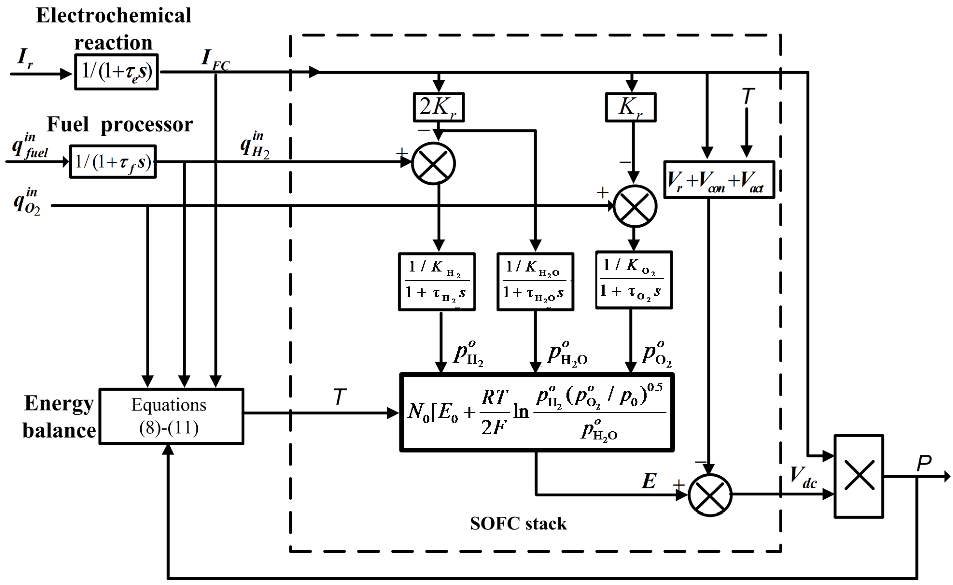
2.1. The SOFC Dynamic Model for Power System Studies

Padullés et al. [21] developed one of the earliest SOFC stack models specifically for power system studies, and the model is shown within the dash lines in Figure 1. In this model, it is assumed the stack temperature T is constant. Considering the cell stack tabular structure, the channels that transport the gases along the electrodes have a fixed volume, but their lengths are small. Hence it is sufficient to define one single pressure value in the cell stack interior. The exhaust of each channel is via a single orifice. The ratio of pressures between the interior and exterior of the channel is large enough and it can be assumed that the orifice is choked and the lumped-parameter model can be derived. Therefore, the mass balance equation, expressed in terms of the partial pressures p_i, is given as,

$$\frac{d{p}_i}{dt}=\frac{RT}{V_i}(q_i^{in}-q_i^o-q_i^r)=\frac{1}{{\text{τ}}_i}[\frac{1}{K_i}(q_i^{in}-q_i^r)-p_i]$$

(1)

where the subscript “i” denotes either H₂, O₂ or water (H₂O); the superscript “in”, “o” and “r” denote the input, output and reaction variable, respectively; R is the ideal gas constant; V_i is the anode or cathode volume; and q_i, K_i and τ_i are the ith gas mole flow rate, valve molar constant and time constant, respectively. Thus, τ_i can be written as,

$${\text{τ}}_i=V_i/(K_{i}RT)$$

(2)

According to the Faraday’s Law of Electrolysis, the reaction flow rates are,

$$q_{{\text{H}}_2}^r=2q_{{\text{O}}_2}^r=-q_{{\text{H}}_{2}O}^r=2K_r{I}_{FC}$$

(3)

where K_r = N₀/(4F); N₀ is the number of the cells connected in series in the stack; F is the Faraday constant of 96,485 C·mol⁻¹; and I_FC is the stack current.

In order to improve the SOFC model, Zhu and Tomsovic included the dynamics of the electrochemical reaction and the fuel processor [22]. In Figure 1, these processes are represented by two first-order equations,

$$d{I}_{FC}/dt=(I_r-I_{FC})/{\text{τ}}_e$$

(4)

$$d{q}_{{\text{H}}_2}^{in}/dt=(q_{fuel}^{in}-q_{{\text{H}}_2}^{in})/{\text{τ}}_f$$

(5)

where I_r is the reference stack current; $q_{fuel}^{in}$ is the natural gas input; τ_e and τ_f are the respective process time constants.

It can be seen from Equations (1)–(2) that the partial pressures p_i are dependent on the stack temperature T which has to be carefully controlled as it can affect the cell efficiency, stack reliability and lifespan [5]. In order to improve the accuracy of the stack model, the dynamic behavior of the cell according to T can be derived based on the energy balance principle [30]. The relevant equation is,

$$m_s{C}_{ps}dT/dt={\displaystyle \sum q_i^{in}({\overline{h}}_i^{in}}-{\overline{h}}_i^o)+{\displaystyle \sum q_i^r{\overline{h}}_i^o}-P$$

(6)

where P is the SOFC dc output power; m_sC_ps is the mass-specific heat product of the stack; ${\overline{h}}_i$ is the ith gas per mole enthalpy and it can be written as,

$${\overline{h}}_i={\overline{h}}_{i,std}+{\overline{C}}_{pi}\text{Δ}T$$

(7)

In Equation (7), ${\overline{h}}_{i,std}$ is the ith gas per mole enthalpy at the standard pressure of 0.1 MPa and the standard temperature T_std of 283K; ${\overline{C}}_{pi}$ is the ith gas average constant-pressure specific heat; and ΔT is the temperature change.

Figure 1. The benchmark solid oxide fuel cell (SOFC) dynamic model.

Figure 1. The benchmark solid oxide fuel cell (SOFC) dynamic model.

Substituting Equations (3) and (7) into Equation (6), Equation (6) can be rewritten as,

$$dT/dt=(A/B-T-P/B)/{\text{τ}}_T$$

(8)

where

$$\begin{array}{l}A=[{\overline{C}}_{p{\text{H}}_2}{q}_{{\text{H}}_2}^{in}+({\overline{C}}_{p{\text{O}}_2}+k_c{\overline{C}}_{p{\text{N}}_2})q_{{\text{O}}_2}^{in}]T_{in}\\ -K_r{I}_{FC}{T}_{std}(2{\overline{C}}_{p{\text{H}}_2}{q}_{{\text{H}}_2}^{in}+{\overline{C}}_{p{\text{O}}_2}-2{\overline{C}}_{p{\text{H}}_2\text{O}})-2K_r{I}_{FC}{H}_{LHV}\end{array}$$

(9)

$$B={\overline{C}}_{p{\text{H}}_2}(q_{{\text{H}}_2}^{in}-2K_r{I}_{FC})+{\overline{C}}_{p{\text{O}}_2}(q_{{\text{O}}_2}^{in}-K_r{I}_{FC})+2K_r{I}_{FC}{\overline{C}}_{p{\text{H}}_{2}O}+k_c{\overline{C}}_{p{\text{N}}_2}{q}_{{\text{O}}_2}^{in}$$

(10)

$${\text{τ}}_T=m_s{C}_{ps}/B$$

(11)

In Equation (9), H_LHV has the low heat value of 241.83 kJ if 1 mole of H₂ is fully combusted to produce gaseous H₂O at the standard state [1]; and T_in is the stack inlet gas temperature. As $q_{{\text{H}}_2}^{in}$ > 2 K_rI_FC and $q_{{\text{O}}_2}^{in}$ > K_rI_FC, B given by Equation (10) is positive and it will increase with I_FC. Therefore, the stack temperature time constant τ_T shown in Equation (11) will be minimal when the SOFC is at the highest load condition.

The response speed of the electrochemical, mass transfer and thermodynamic processes in the SOFC are characterized by the time constants τ_e, τ_i, τ_f and τ_T. This observation is used in the design of the hierarchical control scheme.

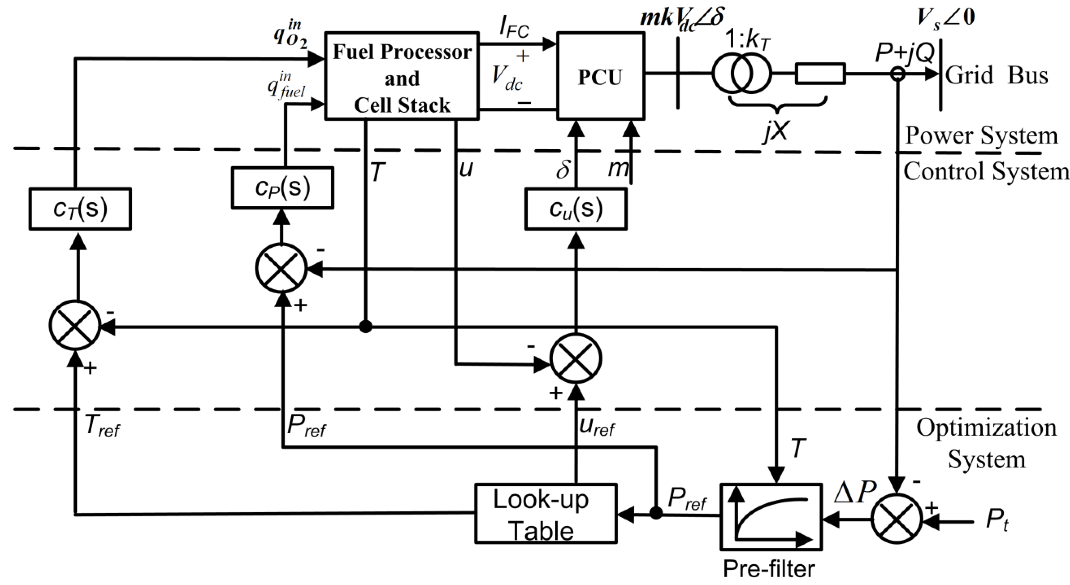
2.2. Power Regulation of a Grid-Connected SOFC

Figure 2 schematically shows a SOFC operating under the grid-connected condition. The PCU provides the required dc/ac interface. Typically, power electronics switching devices in the PCU are controlled using the Sinusoidal Pulse Width Modulation (SPWM) technique. The modulation index (m) and the phase shift angle (δ) are the two control variables associated with this technique. The remaining “Control and Optimization Systems” parts are described in later sections.

Figure 2. Schematic diagram of a grid-connected SOFC power plant and the overall load tracking control system for maximum electrical efficiency operation.

Figure 2. Schematic diagram of a grid-connected SOFC power plant and the overall load tracking control system for maximum electrical efficiency operation.

Denote the terminal voltage of the SOFC stack as V_dc and the grid voltage as V_s. The turns-ratio of the transformer is 1:k_T, and the transformer series impedance plus the linking feeder yield the equivalent reactance X. Define $k=\sqrt{3}/(2\sqrt{2})k_T$. The injected active and reactive power (P + jQ) from the SOFC to the grid system is [27],

$$P=mk{V}_{dc}{V}_s\text{sin}\mathrm{\delta }/X$$

(12)

$$Q=(mk{V}_{dc}{V}_s\text{cos}\mathrm{\delta }-V_s^2)/X$$

(13)

From Figure 1 and Figure 2, it is seen that the grid-connected SOFC power plant has four control variables, namely $q_{fuel}^{in}$, $q_{{\text{O}}_2}^{in}$, m and δ. As Q is strongly dependent on m, m is therefore often manipulated to allow the SOFC power plant to operate under constant voltage, constant reactive power or constant power factor operating schemes. The present investigation, however, focuses on the active power control. Accordingly, the SOFC power plant terminal is treated as a PV bus. In addition, if the switching losses in the PCU and in the feeder are ignored, I_FC can be regulated through m and δ [27],

$$I_{FC}=mk{V}_s\text{sin}\mathrm{\delta }/X$$

(14)

2.3. Operating Variables and Constraints

The operating variables of the grid-connected SOFC such as T, V_dc, P, $q_{{\text{H}}_2}^{in}$, $q_{{\text{O}}_2}^{in}$ and I_r (I_FC) can be calculated based on the energy balance principle, Nernst equation and Figure 1, i.e., through solving the following equations,

$${\displaystyle \sum q_i^{in}({\overline{h}}_i^{in}}-{\overline{h}}_i^o)+{\displaystyle \sum q_i^r{\overline{h}}_i^o}=P$$

(15)

$$V_{dc}=N_0[E_0+\frac{RT}{2F}\text{ln}\frac{p_{{\text{H}}_2}^o{(p_{{\text{O}}_2}^o/p_0)}^{0.5}}{p_{{\text{H}}_2\text{O}}^o}]-V_{act}-V_r-V_{con}$$

(16)

$$P=V_{dc}{I}_{FC}$$

(17)

where E₀, the ideal standard potential, is a function of T [30],

$$E_0=1.2856+0.000252 T$$

(18)

In Equation (16), p₀ is the standard pressure. V_act, V_r and V_con, as shown in Equations (19)–(21), are activation loss, Ohmic loss and concentration loss, respectively [1]. The detailed definitions of the parameters and their typical values are given in Nomenclature and Table 1

$$V_{act}=a+b\text{log}{I}_{FC}$$

(19)

$$V_r=\mathrm{\alpha }\text{exp}[\mathrm{\beta }(1/T_{in}-1/T)]I_{FC}$$

(20)

$$V_{con}=RT/(2F)\cdot \text{ln}(1-I_{FC}/I_L)$$

(21)

Among the six steady-state operating variables T, V_dc, P, $q_{{\text{H}}_2}^{in}$, $q_{{\text{O}}_2}^{in}$ and I_r (I_FC), if any three of them are given, the other three can be obtained by solving the nonlinear Equations (15)–(17).

The cell lifespan and performance are dependent on the operating parameters. Therefore, three operating constraints must be respected for the safe operation of the cell. The most important operating constraint is the fuel utilization factor u, given as,

$$u=2K_r{I}_{FC}/q_{{\text{H}}_2}^{in}$$

(22)

$$u_{\text{min}}\le u\le u_{\text{max}}$$

(23)

Typically, u_min = 0.7 and u_max = 0.9 [21].

The other two operating constraints are T and P,

$$T_{\text{min}}\le T\le T_{\text{max}}$$

(24)

$$P_{\text{min}}\le P\le P_{\text{max}}$$

(25)

Typically, T_min = 1173 K, T_max = 1273 K, P_min = 0.1 pu and P_max = 1 pu of the SOFC rated power [1,23].

2.4. Determination of the Optimal Operating Condition

The electrical efficiency η of the hydrogen SOFC is defined as the ratio of the net power to the total power obtainable by burning H₂ at the standard state [1],

$$\eta =(P-P_{loss})/(q_{{\text{H}}_2}^{in}{H}_{LHV})$$

(26)

However, if the stack operating pressure p is higher than 0.1 MPa, not all the power generated by the SOFC will be delivered to the external circuit. The parasitic losses P_loss is dominated by the air compressor in the form [1],

$$P_{loss}={\overline{C}}_{pair}{T}_{std}(p^{0.286}-1)(1+k_c)q_{{\text{O}}_2}^{in}/{\mathrm{\eta }}_c$$

(27)

where η_c is the equivalent efficiency of the air compressor.

Under a given pressure p, it can be seen from Equations (26) and (27) that η is the function of P, $q_{H_2}^{in}$, and $q_{{\text{O}}_2}^{in}$. There is one set of operating variables which enables the SOFC to operate at the maximum electrical efficiency η_max. In order to optimize η, a nonlinear programming problem (NLPP) is formulated as follows,

Objective function

$$\text{ Maximize }\mathrm{\eta }$$

(28)

Subject to

$$\begin{array}{l}\text{Equality constraints (15)-(17)}\\ \text{Inequality constraints (23)-(25)}\end{array}$$

(29)

The optimization is obtained by treating P, $q_{H_2}^{in}$ and $q_{O_2}^{in}$ as the decision variables in the NLPP. Numerical optimization software packages such as that provided by MATLAB can be used to search η_max. At the end of the NLPP search, the optimal set of T, V_dc, $q_{O_2}^{in}$ $q_{H_2}^{in}$, I_r (I_FC) as well as u for a targeted P will be obtained and pre-stored in a look-up table as the reference input signals for the SOFC load tracking control system.

3. Hierarchical Load Tracking Control Scheme for the Grid-Connected SOFC

With the optimal operating condition of the SOFC determined by the NLPP, the load tracking control scheme for the grid-connected SOFC can be developed to track the power demand and operate at η_max.

The open-loop poles of the SOFC are analyzed to study the dynamic response of the SOFC and a hierarchical control scheme for the SOFC is proposed based on the dynamic response analysis.

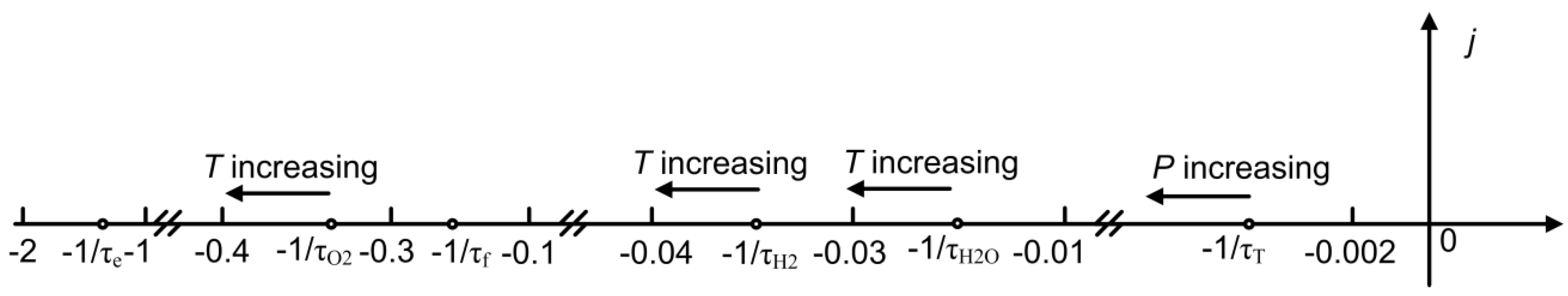
3.1. Analysis of the Open-Loop System Poles

In the load tracking control scheme for the SOFC, the internal dynamics of the PCU can be neglected as the typical response time of the PCU is a few milliseconds. The load tracking speed of the SOFC will be dominated by the dynamic response of devices on the dc side of the power plant where the typical time constants are of the order of 1s or larger.

The response characteristics of the SOFC operating at the maximum efficiency can be assessed by examining the locations of the six open-loop poles of the dynamic model shown in Figure 1. The ith pole can be calculated as,

$$s_i=-1/{\text{τ}}_i$$

(30)

The electrochemical reaction and fuel processor contribute to the poles −1/τ_e and −1/τ_f. They are independent of P and T. However, the location of the poles $-1/{\tau }_{H_2}$, $-1/{\tau }_{O_2}$, $-1/{\tau }_{H_{2}O}$ and −1/τ_T may change when the SOFC operates at different power levels. As shown in Equation (2) and Figure 3, three gas time constants are the function of T but independent of I_FC. Therefore, $-1/{\tau }_{H_2}$, $-1/{\tau }_{O_2}$ and $-1/{\tau }_{H_{2}O}$ will be away from the origin when T increases. On the other hand, from Equations (10) and (11), τ_T is seen to be inversely proportional to I_FC. Thus, the remaining pole −1/τ_T is directly proportional to I_FC or P.

Figure 3. Illustrative of the positions of the six poles of the dynamic model.

Figure 3. Illustrative of the positions of the six poles of the dynamic model.

When the SOFC operates at η_max, the poles can be divided into two groups: plotted in Figure 3, the distance of the pole −1/τ_T to the imaginary axis is at least six times smaller than that of the other five poles. The observation on the locations of the open-loop poles shall be used to develop the structure of the hierarchical load tracking and temperature control scheme for the SOFC.

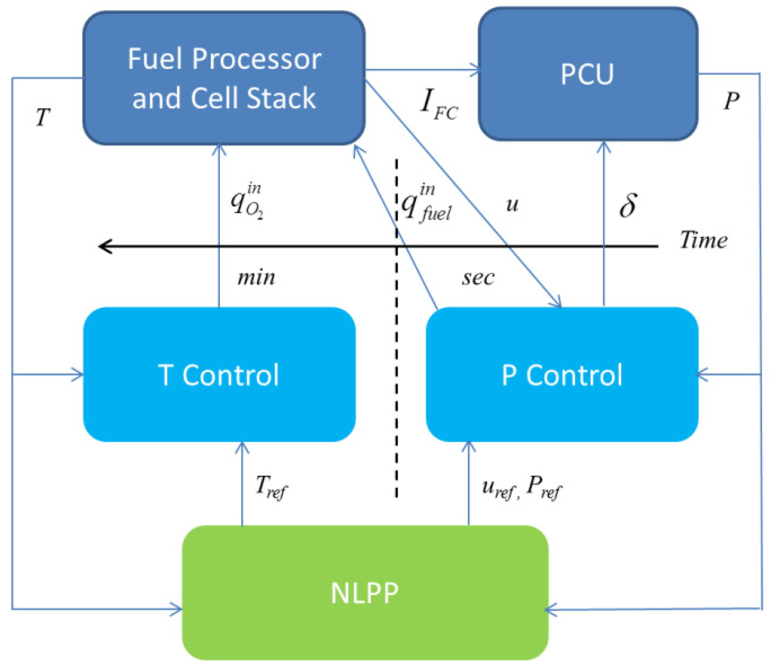
3.2. The Hierarchical Load Tracking Control Scheme

Figure 2 shows that $q_{fuel}^{in}$, $q_{O_2}^{in}$, m and δ can be used to regulate the SOFC output active and reactive power. In the design of a control system for a multi-input-multi-output plant, it is desirable that the structure of the control system is selected in such a way that possible interactions between the control loops is minimized. The modulation index m of the PCU can be used to control the bi-directional reactive power flow to the grid and this can be accomplished in a few milliseconds. Therefore, among the four control variables, m can be treated as a quasi-steady state variable during the load tracking process because the electrochemical, mass transfer and thermodynamics processes usually takes a much longer period.

Based on the observation on the locations of the open-loop poles, it can be concluded that the pole −1/τ_T essentially governs the dynamics of the stack temperature T whereas the load tracking process is dominated by the remaining poles. The T control typically lasts for tens of seconds. Therefore, T can be assumed to be constant for the load tracking operation. On the other hand, by adopting the practice of [29,30,31] in which O₂ was used as a coolant to regulate T, the oxygen flow rate $q_{O_2}^{in}$ can be manipulated such that T is maintained at the optimal value to realize the SOFC η_max operation. It therefore results in a single-input-single-output (SISO) stack temperature control scheme, denoted as the T control system in this paper. With the T control in place, the remaining two control variables $q_{fuel}^{in}$ and δ can be utilized to perform the load tracking of P while maintaining u at the optimal value. This strategy leads to a two-input-two-output P control system.

In summary, as shown in Figure 4, a hierarchical control structure is proposed to achieve both the maximum electrical efficiency operation and stack temperature control of the SOFC when the FC tracks the power demand. The structure is based on the inherent differences in the speeds of response of P, u and T of the SOFC to the demand changes. P and u can be controlled by regulating the control variables $q_{fuel}^{in}$ and δ while T is to be controlled through regulating $q_{O_2}^{in}$, subject to the operating constraints Equations (23)–(25). The proposed hierarchical control structure is more comprehensive, in comparison with the on-line load tracking scheme shown in [27] in which T is assumed constant.

Figure 4. Diagram of the hierarchical control scheme.

Figure 4. Diagram of the hierarchical control scheme.

4. Design of the P and T Control Systems

The detailed design procedure of the P and T control systems is described in this section.

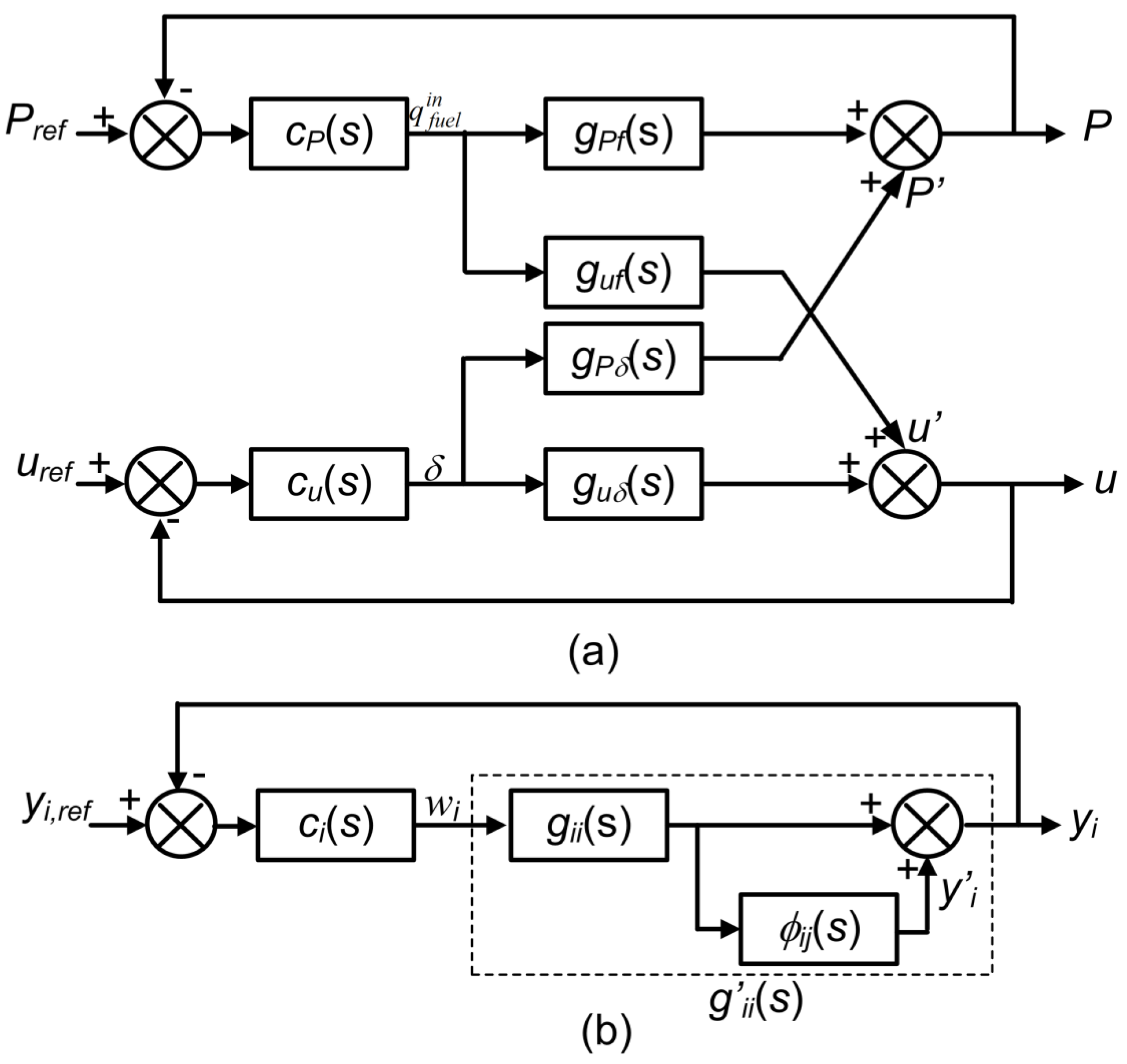
4.1. SOFC Dynamic Model for the Design of P Controller

According to Section 3.2, T can be assumed constant during the P control process. Therefore, the nonlinear model given in Figure 1 can be linearized around the plant initial operating state. For the convenience of the analysis and controller design, the plant variables are normalized in the following way. The values of the state variables $q_{fuel,\text{max}}^{in}$, u_max, P_max, δ_max, which correspond to the operating condition when the SOFC operates at the maximum P, are selected as the base for the normalization. The normalized output-control model shall be of the form

$$y(s)=G_P(s)w(s)=\left(\begin{array}{cc}{g}_{P\text{δ}}(s)& g_{Pf}(s)\\ g_{u\text{δ}}(s)& g_{uf}(s)\end{array}\right)w(s)$$

(31)

where $y={[\text{Δ}P,\text{Δ}u]}^T$ and $w={[\text{Δ}\mathrm{\delta },\text{Δ}{q}_{fuel}^{in}]}^T$ are the small deviations of the output and control variables. G_P(s) is the transfer function determined by taking the small signal form of Equations (1), (4), (5), (14), (16)–(22). Algebraic manipulation shall yield the following expressions for the various elements in G_P(s):

$$g_{P\mathrm{\delta }}(s)=[P_0+\frac{I_{r,0}^2(g_E-g_V)}{1+{\text{τ}}_{e}s}]\frac{ctg{\mathrm{\delta }}_0{\mathrm{\delta }}_{\text{max}}}{P_{\text{max}}}$$

(32)

$$g_{Pf}(s)=\frac{R{T}_0{u}_0}{1-u_0}\frac{1}{(1+{\text{τ}}_{e}s)(1+{\text{τ}}_{f}s)}\frac{q_{fuel,\text{max}}^{in}}{P_{\text{max}}}$$

(33)

$$g_{u\mathrm{\delta }}(s)=\frac{u_{0}ctg{\mathrm{\delta }}_0}{1+{\text{τ}}_{e}s}\frac{{\mathrm{\delta }}_{\text{max}}}{u_{\text{max}}}$$

(34)

$$g_{uf}(s)=\frac{-u_0^2}{2K_r{I}_{r,0}}\frac{1}{1+{\text{τ}}_{e}s}\frac{q_{fuel,\text{max}}^{in}}{u_{\text{max}}}$$

(35)

where

$$g_E(s)=-\frac{N_{0}R{T}_0}{2F}(\frac{2K_r}{q_{fuel,0}^{in}-2K_r{I}_{r,0}}\frac{1}{1+{\text{τ}}_{H_2}s}+\frac{1}{I_{r,0}}\frac{1}{1+{\text{τ}}_{H_{2}O}s}+\frac{K_r}{2(q_{O_{2,0}}^{in}-K_r{I}_{r,0})}\frac{1}{1+{\text{τ}}_{O_2}s})$$

(36)

$$g_V(s)=\frac{b}{I_{r,0}}+\mathrm{\alpha }\text{exp}[\mathrm{\beta }(\frac{1}{T_{in}}-\frac{1}{T_0})]-\frac{R{T}_0}{2F}\frac{1}{I_L-I_{r,0}}$$

(37)

The subscript “0” in Equations (32)–(37) indicates the initial value of the respective variables when the SOFC operates at η_max.

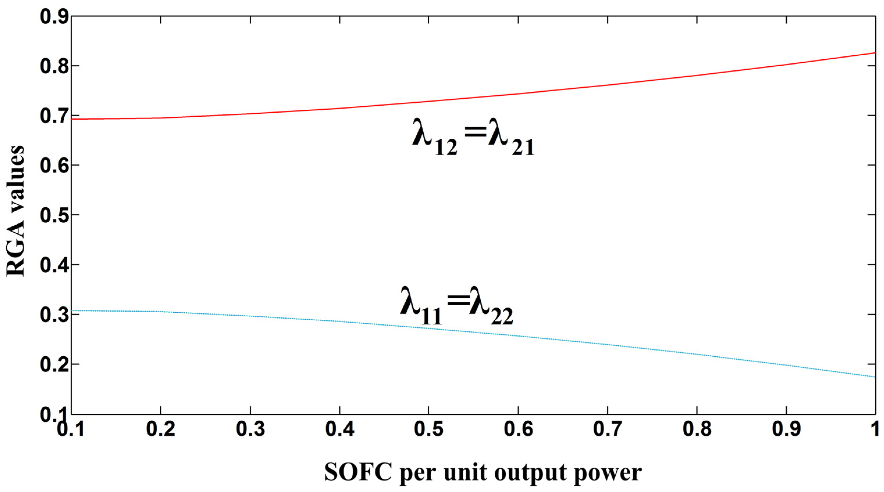
4.2. Selection of P Control Output-input Variables Pairs

Although there are many methods of designing a control system for a general two-input-two-output plant, the decentralized control is a widely used approach. The advantages of the decentralized control include hardware simplicity, operation flexibility, and the relative ease in the controller design and tuning. However, the dynamic performance of the resulting two SISO sub-systems may be degraded by any unaccounted interactions between the two control loops. Therefore, in order to design a feasible and robust controller, an important step is to determine the most suitable two output-input variable pairs for the two SISO sub-systems.

The relative gain array (RGA) is an established technique to measure the steady-state interactions between multiple SISO loops [32]. In the design of the P control system, there are two possible selections of output-input variable pairs: the (P − δ, u − $q_{fuel}^{in}$) pair and the (P − $q_{fuel}^{in}$, u − δ) pair. The most suitable output-input variables pair shall be examined by observing the relative steady state gain between the inputs and outputs. Define the RGA matrix Λ of the plant Equation (31) as the Hadamard product of G_P(0) and its inverse transposition,

$$\mathrm{\Lambda }=G_P(0)\circ G_P^{-T}(0)$$

(38)

With the typical values given in Table 1 and the SOFC operating at η_max, the variations of each element of Λ are shown in Figure 5. It is shown that the values of the off-diagonal elements λ₁₂ and λ₂₁ are closer to 1 compared to that of the diagonal elements λ₁₁ and λ₂₂, particularly under heavy load conditions. This means the selection of the output-input pair (P − $q_{fuel}^{in}$, u − δ) will be more suitable because the interactions of the P − δ and u − $q_{fuel}^{in}$ loops are smaller and decreases as P increases. Therefore, (P − $q_{fuel}^{in}$, u − δ) were selected as the output-input variable pairs when designing the P control system.

Figure 5. Variations of the values of Λ elements with P.

Figure 5. Variations of the values of Λ elements with P.

4.3. Design of the Decentralized P Controller

Figure 6a shows the P control block diagram where an input variable with the subscript “ref” denotes its reference value. The figure has been configured to reflect the outcome of the pair selection described in the previous sub-section, i.e., the adoption of the (P − $q_{fuel}^{in}$, u − δ) output-input variable pairs. The system in Figure 6a is then split into two independent SISO systems, with each SISO having the structure shown in Figure 6b. The so-called multiplicate model factor (MMF) is utilized to account for the loop interactions between the two SISO systems. In Figure 6b, c_i(s) is the respective controller where the subscript “i” denotes either P or u. The design method for c_i(s) can be summarized as follows.

Step One: Design the c_i(s) controllers without considering loop interactions. Suppose the controller c_i(s) in Figure 6b is the PID type and is tuned using the simple internal mode control (SIMC) method described in [32]. Thus, for a second-order system g_ii(s) with a dc-gain k_i and a time delay θ_i:

$$g_{ii}(s)=k_i{e}^{-{\mathrm{\theta }}_{i}s}{[({\text{τ}}_{i}s+1)({\text{τ}}_i^{\text{'}}s+1)]}^{-1};{\text{τ}}_i>{\text{τ}}_i^{\text{'}};{\mathrm{\theta }}_i>0$$

(39)

c_i(s) shall be of the form,

$$c_i(s)=k_{pi}(1+1/{\text{τ}}_{ii}s)(1+{\text{τ}}_{di}s)$$

(40)

It can be seen from Equations (33) and (34) that in g_Pf(s) and g_uδ(s), θ_i = 0. Set the desired closed-loop cross-over time constant τ_ci equals to τ_ii, a practice often used in the process control [32], the PID parameter settings are then given as,

$$k_{pi}=1/k_i;{\text{τ}}_{ii}={\text{τ}}_i;{\text{τ}}_{di}={\text{τ}}_i^{\text{'}}$$

(41)

With this set of settings, the phase margin of c_i(s)g_ii(s) is 90° and it meets the typically desirable phase margin of 60°. While it can be seen from Equation (33) that g_Pf(s) is independent of P, however, Equation (34) shows the dc-gain of g_uδ(s) will be the maximum when P = P_min. Therefore, the c_u(s) controller must be designed based on the minimum SOFC output power condition.

Figure 6. P control as applied to: (a) the two-input-two-output SOFC plant model; (b) the individual decentralized SISO plant model.

Figure 6. P control as applied to: (a) the two-input-two-output SOFC plant model; (b) the individual decentralized SISO plant model.

Step Two: Calculate the MMF by using dynamic Relative Index (dRI) and obtain the equivalent transfer function of each SISO system. In Figure 6b, it is shown the output of the sub-system i will be superimposed by the output y’_i from the neighboring system j. Define the dRI between y’_i and the output of the subsystem i as φ_ij(s). φ_ij(s) for the P control system can then be derived using the technique described in [32] for a general process system,

$${\mathrm{\phi }}_{ij}(s)=-g_{ij}(s)g_{ji}(s)g_{ii}^{-1}(s){(c_j^{-1}(s)+g_{jj}(s))}^{-1}$$

(42)

The MMF of the ith SISO system is then given as,

$${\mathrm{\rho }}_i(s)=1+\mathrm{\phi }(s)_{ij}=\left|{\mathrm{\rho }}_i\right|e^{-\text{Δ}{\mathrm{\theta }}_{i}s}$$

(43)

|ρ_i| and ∆θ_i are the magnitude and phase angle of the MMF, respectively. Therefore, the rectangular box formed by the delineated lines in Figure 6b represents the equivalent transfer function g’_ii(s) where

$$g_{ii}^{\text{'}}(s)={\mathrm{\rho }}_i(s)g_{ii}(s)=\left|{\mathrm{\rho }}_i\right|k_i{e}^{-({\mathrm{\theta }}_i+\text{Δ}{\mathrm{\theta }}_i)s}{[({\text{τ}}_{i}s+1)({\text{τ}}_i^{\text{'}}s+1)]}^{-1}$$

(44)

In Equation (44), |ρ_i| and θ_i + ∆θ_i vary with the operating condition of the SOFC. g’_ii(s) can be chosen under the most onerous conditions when both |ρ_i| and θ_i + ∆θ_i have the maximum values, although maximum |ρ_i| and θ_i + ∆θ_i may not necessarily occur under the same operating condition. With this practice,

$${\mathrm{\rho }}_{i,\text{max}}=\text{max}(1,\left|{\mathrm{\rho }}_i\right|);{\mathrm{\theta }}_{i,\text{max}}=\text{max}({\mathrm{\theta }}_i+\text{Δ}{\mathrm{\theta }}_i)$$

(45)

Step Three: Redesign each c_i(s) based on the equivalent transfer function g’_ii(s). In a manner similar to that in designing the SIMC-PID controller in Step One, if the time constant corresponding to the closed-loop cross-over frequency of c_i(s)g’_ii(s) is selected to be the same as the process maximum time constant τ_ci, as suggested in [32], the new controller settings for c_i(s) are,

$$k_{pi}={\text{τ}}_i/[{\mathrm{\rho }}_{i,\text{max}}{k}_i({\text{τ}}_{ci}+{\mathrm{\theta }}_{i,\text{max}})];{\text{τ}}_{ii}=\text{min}({\text{τ}}_i,4({\text{τ}}_{ci}+{\mathrm{\theta }}_{i,\text{max}}));{\text{τ}}_{di}={\text{τ}}_i^{\text{'}}$$

(46)

4.4. T Control System Design

As explained in Section 3.2, the temperature control involves slower dynamics of the hierarchical control system. Since the SOFC output power P can be maintained at the targeted value through the regulation of the faster P − $q_{fuel}^{in}$, and u − δ control loops, P can be assumed to have reached a quasi-steady state value, even before the T control loop starts to become active. From Equations (8)–(11) and Figure 1, selecting $q_{O_2,\text{max}}^{in}$ and T_min as the normalization base, the small-signal perturbation equation of the temperature T is,

$$\text{Δ}T(s)=g_{To}(s)\text{Δ}{q}_{{\text{O}}_2}^{in}=\frac{({\overline{C}}_{p{\text{O}}_2}+k_c{\overline{C}}_{p{\text{N}}_2})(T_{in}-T_0)}{m_s{C}_{ps}s+B}\frac{q_{{{\text{O}}_2}_{,\text{max}}}^{in}}{T_{\text{min}}}\text{Δ}{q}_{{\text{O}}_2}^{in}$$

(47)

The last equation indicates that at steady-state, an increase in $q_{{\text{O}}_2}^{in}$ will lead to a decrease in T because T_in < T₀. However, as explained in Section 2, the parameter B will increase when I_FC increases. As B also appears in the denominator of Equation (47), the consequence is that the phase margin of the transfer function g_To(s) in Equation (47) will be at the minimum when I_FC is at the minimum, i.e., when P = P_min. Therefore, the parameters of the temperature controller c_T(s) can be determined using the same SIMC-PID tuning method as that used in the design of the P controller. c_T(s) is to be tuned under the most onerous condition when the SOFC is at the minimum load.

4.5. Overall Load Tracking and Temperature Control Scheme

The overall control scheme for the SOFC to achieve η_max during the load tracking process is illustrated in the “Control and Optimization System” portion of Figure 2. Based on the above analysis, both P and u will be ahead of T to reach the reference values. It can be seen from Equation (8) and will be illustrated in Section 5 that continuously varying P may lead the transient T to exceed the constraint given in Equation (24). In order to guarantee the cell lifespan, T should be monitored on-line. If the measured T is not within the pre-set band which is close to its operating boundaries, as shown in Figure 2, the “Pre-filter” block will convert the error between the targeted power level P_t and the SOFC output power P into continuous adjustments P_ref. Since the overall control objective of the load tracking is to achieve η_max, the reference signals T_ref and u_ref can be obtained directly from the look-up table. Hence the SOFC shall attempt to operate at η_max as it approaches P_t. The hierarchical control scheme will track P_ref, u_ref and T_ref through the respective controllers c_P(s), c_u(s) and c_T(s).

Table 1. Typical 100 kW SOFC power plant data.

Parameters	Value
Tin	923 K
p	0.15 MPa
N0	384
msCps	1.1 × 104 (J/K)
Kr	9.95 × 10−4mol/(s.A)
KH2	8.32 × 10−6 mol/(s.Pa)
KH2O	2.77 × 10−6 mol/(s.Pa)
KO2	2.49 × 10−5 mol/(s.Pa)
Va	2.3 m3
Vc	0.76 m3
τf	5 s
τe	0.8 s
α	0.02 Ω
β	−2870 K
a	0.05 V
b	0.11 V
IL	800 A
ηc	0.7

Table 1. Typical 100 kW SOFC power plant data.

Parameters	Value
Tin	923 K
p	0.15 MPa
N0	384
msCps	1.1 × 104 (J/K)
Kr	9.95 × 10−4mol/(s.A)
KH2	8.32 × 10−6 mol/(s.Pa)
KH2O	2.77 × 10−6 mol/(s.Pa)
KO2	2.49 × 10−5 mol/(s.Pa)
Va	2.3 m3
Vc	0.76 m3
τf	5 s
τe	0.8 s
α	0.02 Ω
β	−2870 K
a	0.05 V
b	0.11 V
IL	800 A
ηc	0.7

5. Case Studies

The benchmark SOFC power plant in [21,22,30] was used to carry out case studies to illustrate the efficiency of the proposed hierarchical control scheme. The 100 kW power plant is connected to a 400 V ac system and the associated parameters are given in Table 1. On the 400 V and 100 kVA base, the SOFC power plant ac terminal voltage is assumed to be constant at 1.05 pu. It is also assumed that the link reactance X in Figure 2 is 0.05 pu. The simulation tool used is MATLAB/SIMULINK.

5.1. Steady-State η_max Operations

Suppose the SOFC is to operate between 10 kW and 100 kW. Table 2 shows part of the NLPP calculation results. For comparison, like the steady-state operating conditions in [26,27], the efficiencies (η₁) when T = 1273 K and u = 0.8 under different power are also given. Obviously, η_max is higher than η₁. The optimal η can be found on the boundaries of T and u when P is at the low level. The highest η_max is 43.4% when P = 0.3 pu. However, the power consumed by the air compressor is over 15% of the output power if the cell operating pressure is 0.15 MPa. This will cause η_max less than 40% under the maximum output power condition.

Table 2. The maximum efficiency results by nonlinear programming problem (NLPP).

P (kW)	Ploss (kW)	Vdc (V)	$q_{fuel}^{in}$ (mol/s)	$q_{O_2}^{in}$ (mol/s)	T (K)	u	ηmax	η1
10	1.514	269.31	0.082	0.208	1173	0.9	0.427	0.3904
30	4.438	272.06	0.244	0.610	1173	0.9	0.434	0.3973
50	7.560	269.49	0.410	1.040	1173	0.8998	0.428	0.3992
70	10.889	266.08	0.585	1.497	1173	0.8948	0.418	0.3988
90	14.416	261.51	0.771	1.982	1175	0.8885	0.406	0.3973
100	15.906	257.87	0.872	2.187	1184	0.8849	0.399	0.395

Table 2. The maximum efficiency results by nonlinear programming problem (NLPP).

P (kW)	Ploss (kW)	Vdc (V)	$q_{fuel}^{in}$ (mol/s)	$q_{O_2}^{in}$ (mol/s)	T (K)	u	ηmax	η1
10	1.514	269.31	0.082	0.208	1173	0.9	0.427	0.3904
30	4.438	272.06	0.244	0.610	1173	0.9	0.434	0.3973
50	7.560	269.49	0.410	1.040	1173	0.8998	0.428	0.3992
70	10.889	266.08	0.585	1.497	1173	0.8948	0.418	0.3988
90	14.416	261.51	0.771	1.982	1175	0.8885	0.406	0.3973
100	15.906	257.87	0.872	2.187	1184	0.8849	0.399	0.395

5.2. Controller Design

For the controllers design, the u_max, P_max, δ_max, $q_{fuel,\text{max}}^{in}$, $q_{O_2,\text{max}}^{in}$ and T_min are chosen as 0.9, 100 kW, 0.05 rad, 0.872 mol/s, 2.187 mol/s and 1173 K.

Based on the analysis in Section 4.2, the P control system is split into two SISO sub-systems. Analysis in Section 4.3 has identified the minimum output power condition to be the most onerous condition. From Equation (40), if the cross-over time constant of each SISO system is set equal to the maximum τ_ii, the controllers for the P control designed without considering the loop interactions are c_P(s) = 1.237(1 + 1/5 s)(1 + 0.8 s) and c_u(s) = 0.095(1 + 1/0.8 s). This design corresponds to the cross-over time constants of 0.2 s and 1.25 s for the P − $q_{fuel}^{in}$ loop and u − δ loop, respectively.

When P is 0.1pu or 1pu, the corresponding dRI are: ϕ_Pδ,0.1(j0.2) = 1.414(cos16.1° + jsin16.1°); ϕ_Pδ,1(j0.2) = 0.634(cos28.6° − jsin28.6°); ϕ_uf,0.1(j1.25) = 0.443(cos9.5°+jsin9.5°); and ϕ_uf,1(j1.25) = 0.423(cos13.6° + jsin13.6°). The values of ϕ_Pδ,P(.) confirm the most onerous condition under which the P − $q_{fuel}^{in}$ loop interact with the u − δ loop is at the minimum P condition. The values of ϕ_uf,P(.) show that this loop can contribute to the P − $q_{fuel}^{in}$ loop with the largest gain increase, and the maximum phase lag under the minimum and the maximum P conditions, respectively. In order to guarantee satisfactory dynamic performance of the SOFC under possible loop failures for all output power conditions, the corresponding MMF can be selected to be the extreme gain and phase values simultaneously. Thus, based on the above numerical results and using Equation (43), ρ_Pδ = 2.391exp(−0.96 s) and ρ_uf = 1.442exp(0.04 s). The corresponding equivalent transfer function of each SISO system can then be calculated using Equations (44) and (45) to yield g'_Pf(s) = 1.839exp(−0.96 s)/((1 + 1/5 s)(1 + 0.8 s)) and g'_uδ(s) = 15.147/(1 + 0.8 s). From Equation (46), the new P controllers are c_P(s) =0.531(1 +1/5 s)(1 + 0.8 s) and c_u(s) = 0.066(1 + 1/0.8 s).

As discussed in Section 4.4, the controller for the T control system is also designed when P = P_min. Accordingly, the T controller is c_T(s) = −0.64(1 + 1/292 s).

Again, the above three controllers designed for the model shown in Figure 1 indicate the SOFC is feasible for slow load tracking application. The tracking speed is firstly limited by the P controllers. As the cross-over time constant of c_P(s) is around 0.2 s, it will be safe for the SOFC to track the load within this bandwidth. On the other hand, the cross-over time constant of c_T(s) is about 0.0035 s. The T control system is much slower than the P control system. As shown in Equation (8), the continuing output power change will cause T deviate from the acceptable value. Therefore, the load tracking speed must be slow down until T can be effectively regulated within the constraints.

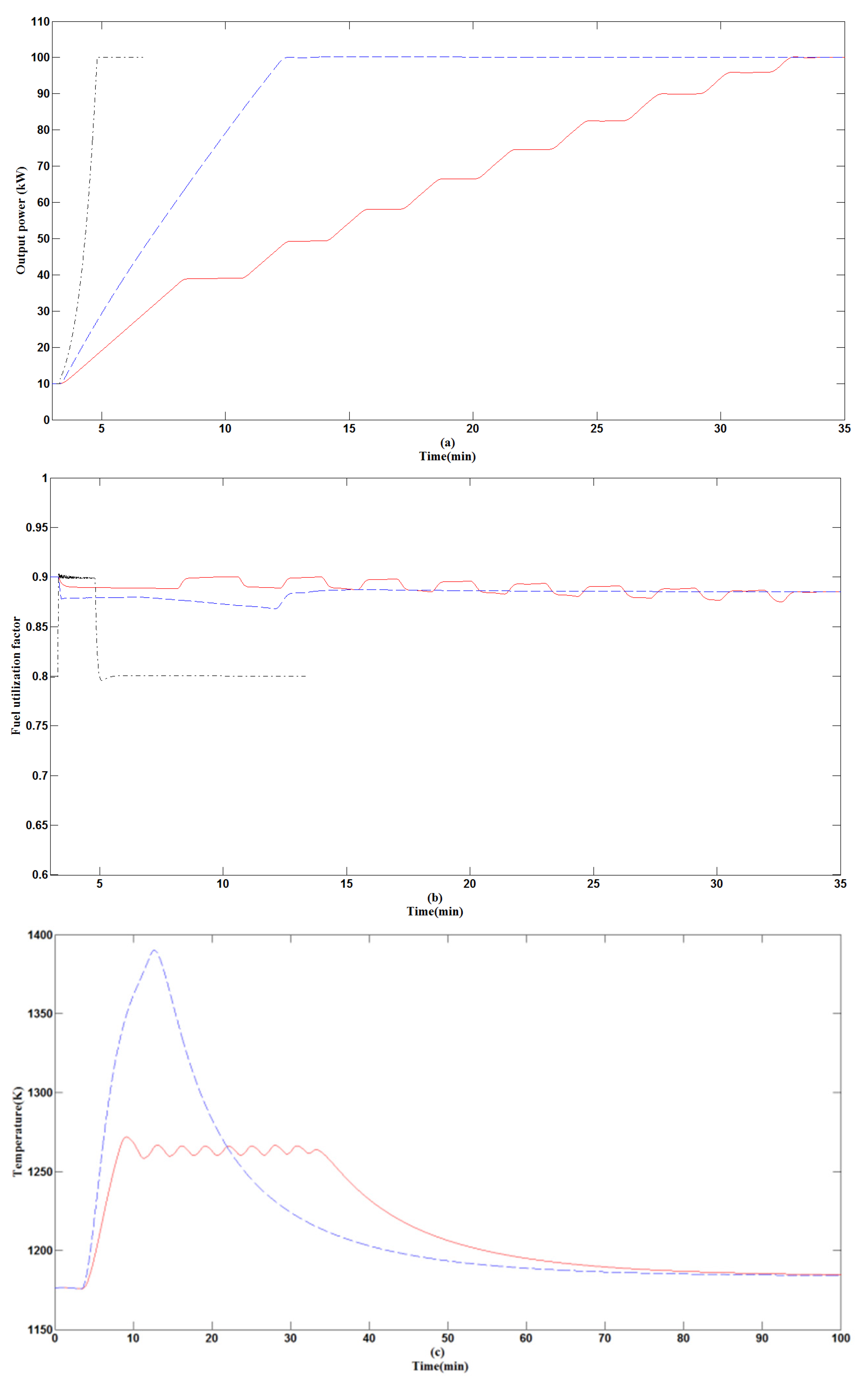
5.3. SOFC Load Tracking Dynamic Performance

This section illustrates the load tracking performance of the SOFC under the proposed hierarchical control scheme with and without considering the temperature control. The results are then compared with that obtained from the on-line control scheme described in [27]. Suppose the power demand increases from 0.1 pu to 1 pu. If the measured T is within the constraints, the load demand on the SOFC can change at the rate of 0.1 pu kW/min. Such load tracking speed is quite close to the results reported in [20,31]. However, as discussed in Section 4.3 and shown in Figure 7a, the “Pre-filter” block can generate the new power reference only the measured T is below a pre-set threshold value (say 1263 K). It will take about 30 min to achieve the targeted power due to the variable power ramp rate. If the temperature control is not considered, the targeted power can be reached in about 12 min. The on-line control strategy proposed in [27] is designed such that the final load level shall be reached within the minimum time. Indeed, the on-line method shown in Figure 7a has a higher speed of response, i.e. the 0.9 pu power change is reached in about 100 s. However, in [27], the ratio of the fuel flow rate to oxygen flow rate is kept constant at 1.145. It is shown in Table 2 that it is impossible to maintain a constant T with the flow rate ratio fixed. Therefore, the constant temperature assumption made in [27] is invalid once the energy balance consideration is included in the dynamic model.

Figure 7. Comparison of SOFC load tracking performance under hierarchical control scheme with considering T bound (──), hierarchical control scheme without considering T bound (---) and on-line control scheme of [27] (-).

Figure 7. Comparison of SOFC load tracking performance under hierarchical control scheme with considering T bound (──), hierarchical control scheme without considering T bound (---) and on-line control scheme of [27] (-).

An interesting observation is that the direction of the u variation based on the on-line method is opposite to that obtained under the hierarchical control. This is shown in Figure 7b. The reason for this is because under the on-line scheme proposed in [27], $q_{fuel}^{in}$ is the only independent control variable and u is kept constant at a pre-set value (which, in this simulation, is 0.8). As derived in [27], $q_{fuel}^{in}$ and u will vary in the same direction following the load change. Under the hierarchical control scheme, however, both $q_{fuel}^{in}$ and δ will affect u. Due to the loop interactions, u will vary in a direction opposite to that of $q_{fuel}^{in}$, as shown in Equation (35). However, the hierarchical control scheme can achieve the optimal value 0.8849, as can be seen in the figure.

From the initial optimal value 1173 K, Figure 7c indicates that it will take about 90 min for the SOFC to reach at 1184 K. T can be maintained under 1273 K during the transient period if T bound is satisfied with the variable load tracking speed. Otherwise, T will be out of the constraint due to the continuously increasing P.

According to the discussion above, it can be concluded that the proposed hierarchical control scheme will be able to track the power demand in a safe manner, and the mutual loop interactions have been included in the control system design. The scheme will also lead to the maximum electrical efficiency operations of the SOFC.

6. Conclusions

By considering the power loss caused by the air compressor, the maximum electrical efficiency operating conditions of the grid-connected SOFC can be obtained by solving a nonlinear programming problem, which is subject to constraints of stack temperature, fuel utilization factor and output power. In order to accommodate the inherently different dynamical processes within the SOFC, a hierarchical control scheme for the grid-connected SOFC power plant has been proposed. The scheme consists of a P control system and a relatively slower T control system. The case studies verify that the proposed hierarchical control scheme can achieve maximum efficiency load tracking operation for the grid-connected SOFC with the stack temperature bounded within the preset constraints.

The FC-based DG technology is still far from mature. Continuous improvements on the FC performance, durability and making it economically competitive are needed in order to realize its wide application. For power system analysis, the SOFC model and control strategies should be improved and verified through experiment in the future work.

References

1. Larminie, J.; Dicks, A. Fuel Cell System Explained, 2nd ed.; John Wiley: New York, NY, USA, 2002. [Google Scholar]
2. Singhal, S.C.; Kendall, K. High Temperature Solid Oxide Fuel Cells: Fundamentals, Design, and Applications; Elsevier: New York, NY, USA, 2003. [Google Scholar]
3. Zhang, X.; Chan, S.H.; Li, G.; Ho, H.K.; Li, J.; Feng, Z. A review of integration strategies for solid oxide fuel cells. J. Power Sour. 2010, 195, 685–702. [Google Scholar] [CrossRef]
4. Park, S.K.; Ahn, J.H.; Kim, T.S. Performance evaluation of integrated gasification solid oxide fuel cell/gas turbine systems including carbon dioxide capture. Appl. Energy 2011, 88, 2976–2987. [Google Scholar] [CrossRef]
5. Razbani, O.; Wærnhus, I.; Assadi, M. Experimental investigation of temperature distribution over a planar solid oxide fuel cell. Appl. Energy 2013, 105, 155–160. [Google Scholar] [CrossRef]
6. Zhu, G.R.; Loo, K.H.; Lai, Y.M.; Tse, C.K. Quasi-maximum efficiency point tracking for direct methanol fuel cell in dmfc-supercapacitor hybrid energy system. IEEE Trans. Energy Convers. 2012, 27, 561–571. [Google Scholar] [CrossRef]
7. Kelouwani, S.; Adegnon, K.; Agbossou, K.; Dube, Y. Online system identification and adaptive control for pem fuel cell maximum efficiency tracking. IEEE Trans. Energy Convers. 2012, 27, 580–592. [Google Scholar] [CrossRef]
8. Hong, W.T.; Yen, T.H.; Chung, T.D.; Huang, C.N.; Chen, B.D. Efficiency analyses of ethanol-fueled solid oxide fuel cell power system. Appl. Energy 2011, 88, 3990–3998. [Google Scholar] [CrossRef]
9. Su, Y.; Chan, L.C.; Shu, L.; Tsui, K.L. Real-time prediction models for output power and efficiency of grid-connected solar photovoltaic systems. Appl. Energy 2012, 93, 319–326. [Google Scholar] [CrossRef]
10. Bhattacharyya, D.; Rengaswamy, R. A reiview of solid oxide fuel cell (sofc) dynamic model. Ind. Eng. Chem. Res. 2009, 48, 6068–6086. [Google Scholar] [CrossRef]
11. Wang, K.; Hissel, D.; Péra, M.C.; Steiner, N.; Marra, D.; Sorrentino, M.; Pianese, C.; Monteverde, M.; Cardone, P.; Saarinen, J. A review on solid oxide fuel cell models. Int. J. Hydrog. Energy 2011, 36, 7212–7228. [Google Scholar] [CrossRef]
12. Huang, B.; Qi, Y.; Murshed, M. Solid oxide fuel cell: Perspective of dynamic modeling and control. J. Process Control 2011, 21, 1426–1437. [Google Scholar] [CrossRef]
13. Spivey, B.J.; Edgar, T.F. Dynamic modeling, simulation, and mimo predictive control of a tubular solid oxide fuel cell. J. Process Control 2012, 22, 1502–1520. [Google Scholar] [CrossRef]
14. Menon, V.; Janardhanan, V.M.; Tischer, S.; Deutschmann, O. A novel approach to model the transient behavior of solid-oxide fuel cell stacks. J. Power Sources 2012, 214, 227–238. [Google Scholar] [CrossRef]
15. Gao, F.; Simoes, M.G.; Blunier, B.; Miraoui, A. Development of a quasi 2-D modeling of tubular solid-oxide fuel cell for real-time control. IEEE Trans. Energy Convers. 2014, 29, 9–19. [Google Scholar] [CrossRef]
16. Wang, C.; Nehrir, M.H. A physically based dynamic model for solid oxide fuel cells. IEEE Trans. Energy Convers. 2007, 22, 887–897. [Google Scholar] [CrossRef]
17. Sorrentino, M.; Pianese, C.; Guezennec, Y.G. A hierarchical modeling approach to the simulation and control of planar solid oxide fuel cells. J. Power Sour. 2008, 180, 380–392. [Google Scholar] [CrossRef]
18. Huo, H.B.; Wu, Y.X.; Liu, Y.Q.; Gan, S.H.; Kuang, X.H. Control-oriented nonlinear modeling and temperature control for solid oxide fuel cell. J. Fuel Cell Sci. Technol. 2010. [Google Scholar] [CrossRef]
19. Hajimolana, S.A.; Tonekabonimoghadam, S.M.; Hussain, M.A.; Chakrabarti, M.H.; Jayakumar, N.S.; Hashim, M.A. Thermal stress management of a solid oxide fuel cell using neural network predictive control. Energy 2013, 62, 320–329. [Google Scholar] [CrossRef]
20. Komatsu, Y.; Kimijima, S.; Szmyd, J.S. Numerical analysis on dynamic behavior of solid oxide fuel cell with power output control scheme. J. Power Sour. 2013, 223, 232–245. [Google Scholar] [CrossRef]
21. Padulles, J.; Ault, G.W.; McDonald, J.R. An integrated sofc plant dynamic model for power systems simulation. J. Power Sour. 2000, 86, 495–500. [Google Scholar] [CrossRef]
22. Zhu, Y.; Tomsovic, K. Development of models for analyzing the load-following performance of microturbines and fuel cells. Electr. Power Syst. Res. 2002, 62, 1–11. [Google Scholar] [CrossRef]
23. Li, Y.H.; Choi, S.S.; Rajakaruna, S. An analysis of the control and operation of a solid oxide fuel-cell power plant in an isolated system. IEEE Trans. Energy Convers. 2005, 20, 381–387. [Google Scholar] [CrossRef]
24. Li, Y.G.; Shen, J.; Lu, J.H. Constrained model predictive control of a solid oxide fuel cell based on genetic optimization. J. Power Sour. 2011, 196, 5873–5880. [Google Scholar] [CrossRef]
25. Nayeripour, M.; Hoseintabar, M. A new control strategy of solid oxide fuel cell based on coordination between hydrogen fuel flow rate and utilization factor. Renew. Sustain. Energy Rev. 2013, 27, 505–514. [Google Scholar] [CrossRef]
26. Sanandaji, B.M.; Vincent, T.L.; Colclasure, A.M.; Kee, R.J. Modeling and control of tubular solid-oxide fuel cell systems: II. Nonlinear model reduction and model predictive control. J. Power Sour. 2011, 196, 208–217. [Google Scholar] [CrossRef]
27. Li, Y.H.; Rajakaruna, S.; Choi, S.S. Control of a solid oxide fuel cell power plant in a grid-connected system. IEEE Trans. Energy Convers. 2007, 22, 405–413. [Google Scholar] [CrossRef]
28. Du, W.; Wang, H.F.; Zhang, X.F.; Xiao, L.Y. Effect of grid-connected solid oxide fuel cell power generation on power systems small-signal stability. IET Renew. Power Gener. 2012, 6, 24. [Google Scholar] [CrossRef] [Green Version]
29. Sorrentino, M.; Pianese, C. Model-based development of low-level control strategies for transient operation of solid oxide fuel cell systems. J. Power Sour. 2011, 196, 9036–9045. [Google Scholar] [CrossRef]
30. Vijay, P.; Tade, M.O.; Datta, R. Effect of the operating strategy of a solid oxide fuel cell on the effectiveness of decentralized linear controllers. Ind. Eng. Chem. Res. 2011, 50, 1439–1452. [Google Scholar] [CrossRef]
31. Bunin, G.A.; Wuillemin, Z.; Francois, G.; Nakajo, A.; Tsikonis, L.; Bonvin, D. Experimental real-time optimization of a solid oxide fuel cell stack via constraint adaptation. Energy 2012, 39, 54–62. [Google Scholar] [CrossRef]
32. Wang, Q.G.; Ye, Z.; Cai, W.J.; Hang, C.C. Pid Control for Multivariable Processes; Springer: Berlin, Germany, 2009. [Google Scholar]