
Thermoeconomic Optimization of a Renewable Polygeneration System Serving a Small Isolated Community

 ,
,
Abstract
:1. Introduction
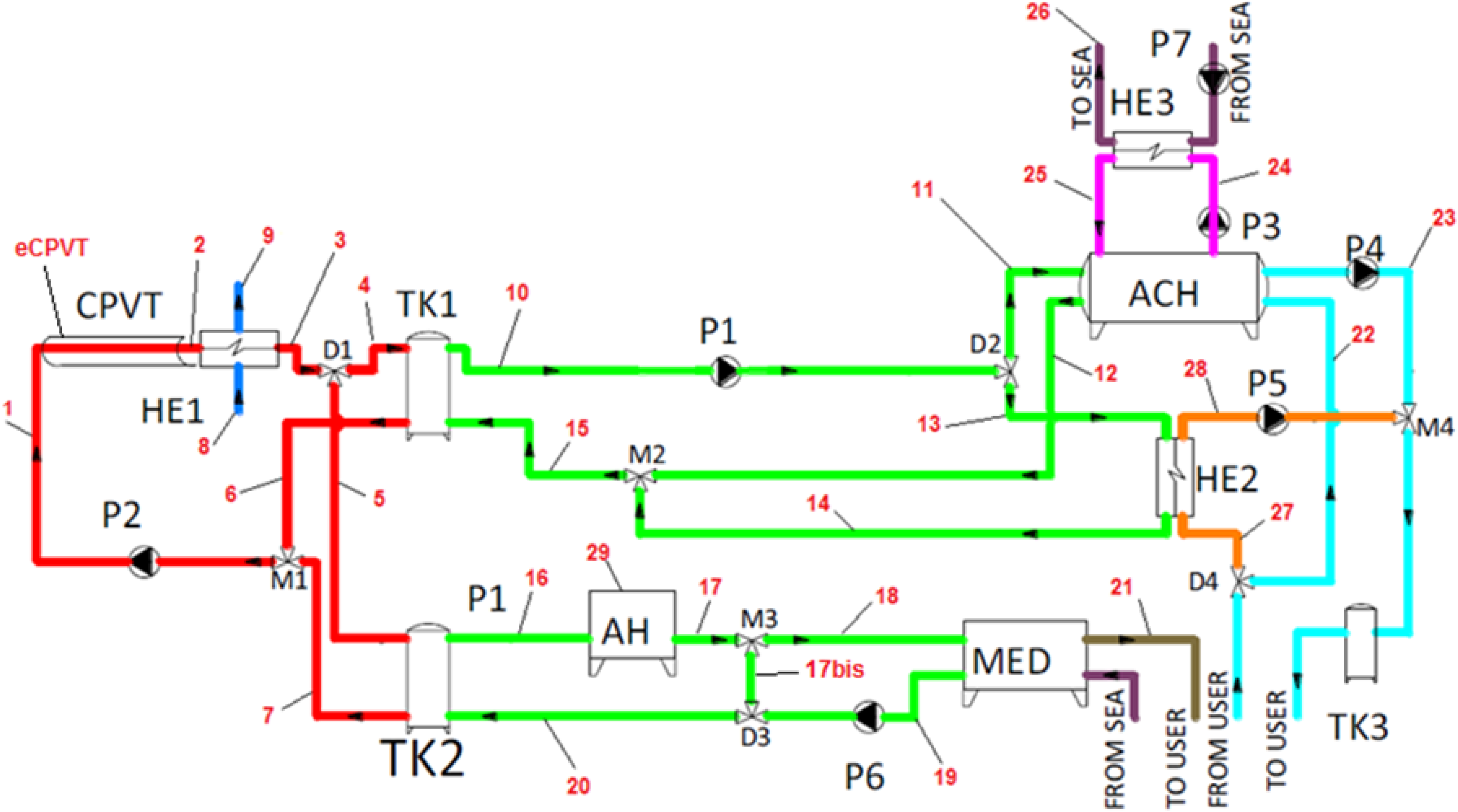
2. System Layout

- (1)
- Solar Collector Fluid, (red line in Figure 1), SCF: pressurized water flowing from the source sides of the tanks to the solar field;
- (2)
- Hot Fluid, (green line in Figure 1), HF: pressurized water flowing from the load sides of the tanks to the devices using solar thermal energy;
- (3)
- Cooling Water, (fuchsia line in Figure 1), CW: water flowing in the condenser and absorber of the Absorption Chiller (ACH);
- (4)
- Chilled Water, (sky blue line in Figure 1), CHW: water flowing in the evaporator of the Absorption Chiller (ACH);
- (5)
- Domestic Hot Water, (orange line in Figure 1), DHW: water supplying sanitary devices;
- (6)
- Hot Water, HW: water supplying space heating devices;
- (7)
- Sea Water, (violet line in Figure 1), SW: water supplied to the MED, in order to be desalinated, or to the heat exchanger used for cooling the ACH;
- (8)
- Desalinated Water, (brown line in Figure 1), DW: fresh water produced by the MED and supplied to final users.
- a Solar Collector field, CPVT, consisting of concentrating parabolic trough solar collectors whose absorber is covered by a triple-junction PV layer; the beam radiation is concentrated on a triangular receiver, placed on the focus of the parabola, on which a multi-junction PV panel is laminated; the triangular receiver is equipped with an internal tube, in which a cooling fluid flows; the system is also equipped with a one-axis tracking system, typical of parabolic trough solar thermal collectors; the PVT can operate up to 100 °C;
- a Thermal Storage system (TK1), supplying heat for space heating and cooling purposes, consisting of a set of stratified vertical hot storage tanks, equipped with inlet stratification devices: the entering position of the inlet fluid is varied so that fluid and tank temperature are equal;
- a Thermal Storage system (TK2), supplying heat for seawater desalination, consisting of a set of stratified vertical hot storage tanks, equipped with inlet stratification devices: the entering position of the inlet fluid is varied so that fluid and tank temperature are equal;
- a plate-fin heat exchanger in the solar loop (HE1), used to produce Domestic Hot Water when the solar irradiation is higher than the ACH (or the HE2) thermal demand;
- a plate-fin heat exchanger in the HW loop (HE2), transferring heat from the HF to the hot water (CHW) to be supplied to the fan-coils during the winter;
- a plate-fin heat exchanger in the CW/SW loops (HE3), cooling the CW loop using the seawater, SW;
- a LiBr-H2O single-effect absorption chiller (ACH), whose generator is fed by the hot fluid (HF) provided by the solar field; the condenser and the absorber of the ACH are cooled by seawater, through the cooling water loop (CW);
- a Multiple-Effect Distillation (MED) unit, producing desalinated water from seawater;
- a wood-chip fired Auxiliary Heater (AH), providing auxiliary thermal energy to the MED unit;
- some fixed-volume pump (P1, P3, P4, P5, P6 and P7) for the HF, HW, SW, CHW and CW loops;
- a variable-speed pump (P2) for the SCF loop;
- an inertial chilled/hot water storage tank (TK3), included in order to reduce the number of start-up and shut-down events for the absorption chiller ACH;
- some Balance of the Plant (BOP) equipment (the majority not displayed in Figure 1 for sake of simplicity), such as pipes, mixers, diverters, valves, and controllers required for the system operations.
3. Simulation Model
3.1. Exergy Model
3.1.1. CPVT Collector
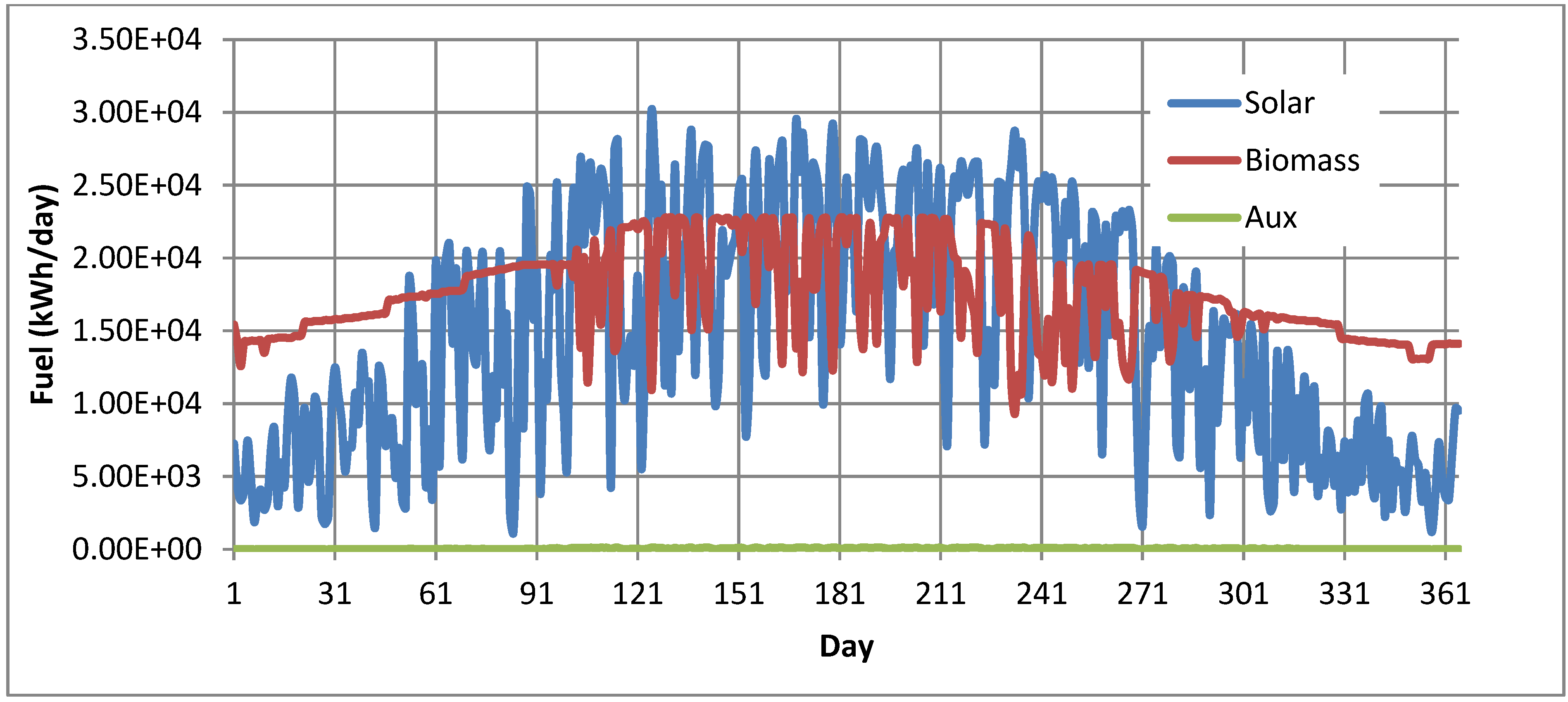
3.1.2. Biomass Heater
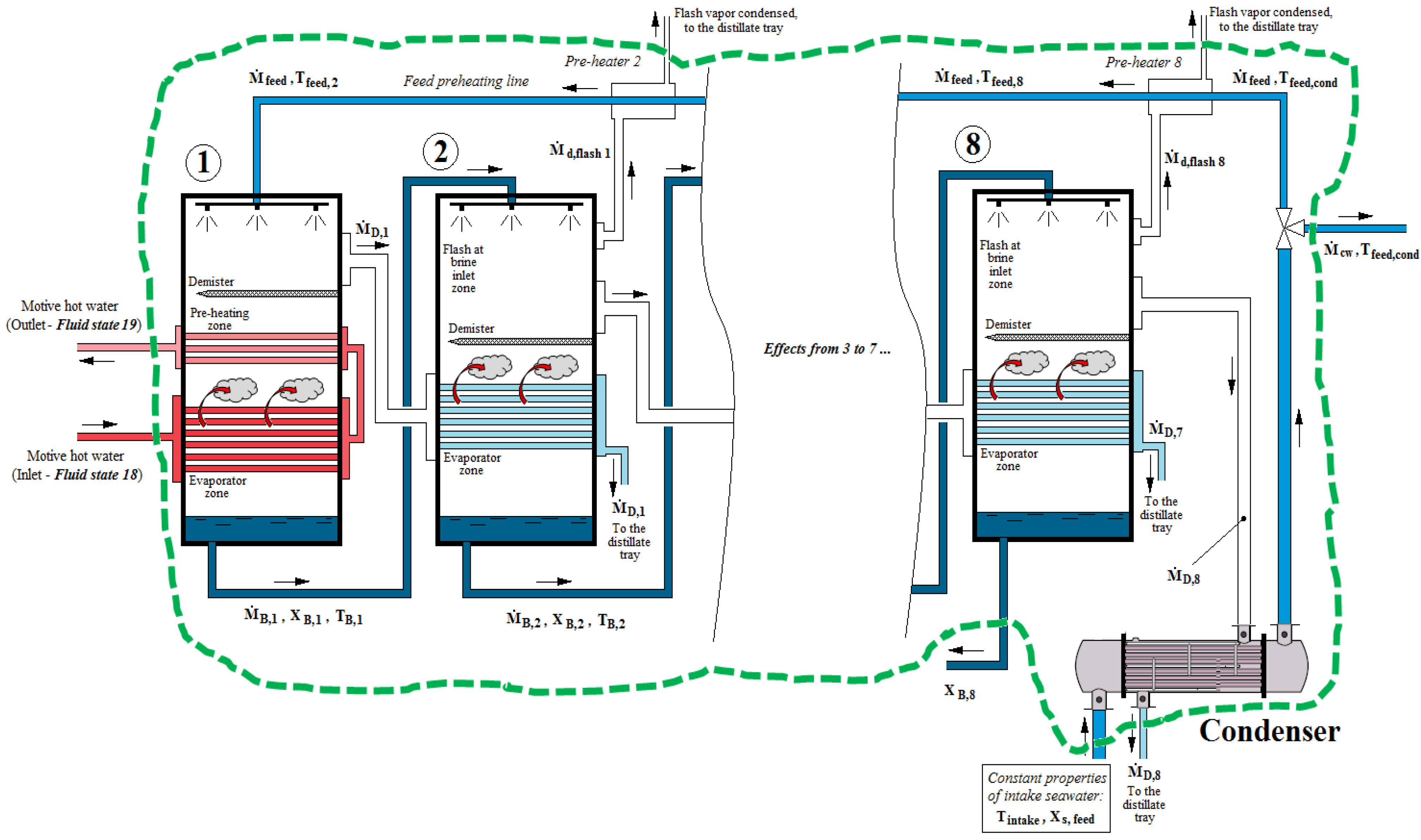
3.1.3. MED
- -
- Motive hot water (i.e., the hot water that supplies heat to the MED unit) entering the 1st effect at conditions represented by thermodynamic state 18 (following the notation in Figure 1) and exiting at state 19. The motive hot water is not involved in any separation process, being then unnecessary to calculate its chemical exergy content that remains constant. The exergy released to the 1st effect is:
- -
- The cooling water that absorbs at the condenser any surplus heat released from the condensing distillate flow that cannot be used to pre-heat the feed. The cooling flow is discarded back to the sea at a temperature Tfeed,cond usually some degrees higher than the intake seawater temperature. Although trivial, calculating the thermal exergy content of this stream is not needed since this exergy flow exiting the boundary volume represents a net loss that, even occurring outside the control volume, can be included in the total exergy balance of the MED unit as any other exergy destruction occurring inside the volume;
- -
- The high salt concentration brine discarded at the last effect, whose chemical exergy flow can be calculated as follows [57].where ωth,0 has been obtained by Equation (13) and ωth,R represents the theoretical minimum work of separation of pure water for finite water recovery ratios, calculated as follows:
3.1.4. Heat Exchangers
3.1.5. Tanks
3.1.6. ACH
3.1.7. RPS
3.2. Economic Model
4. Results and Discussion
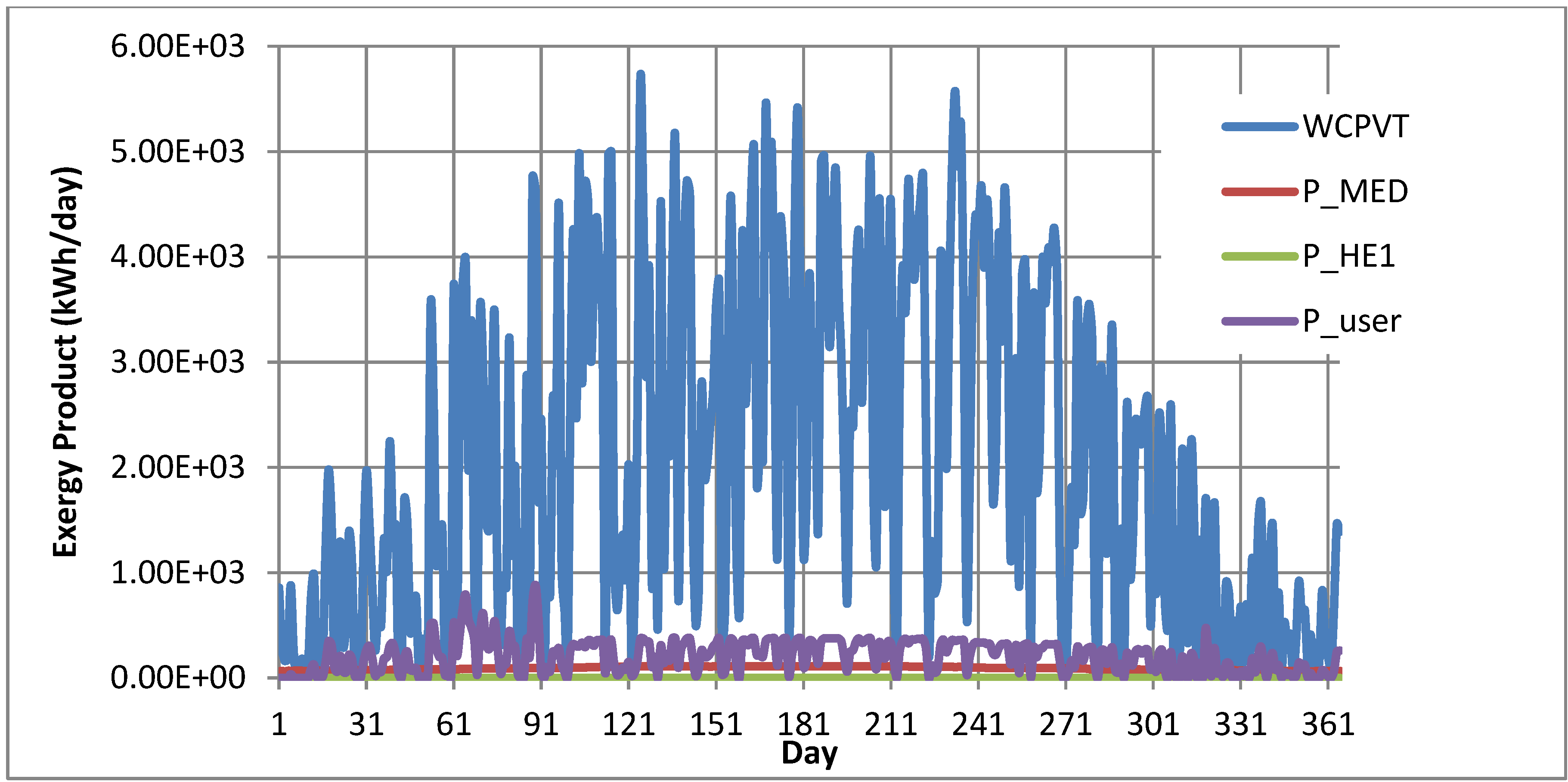
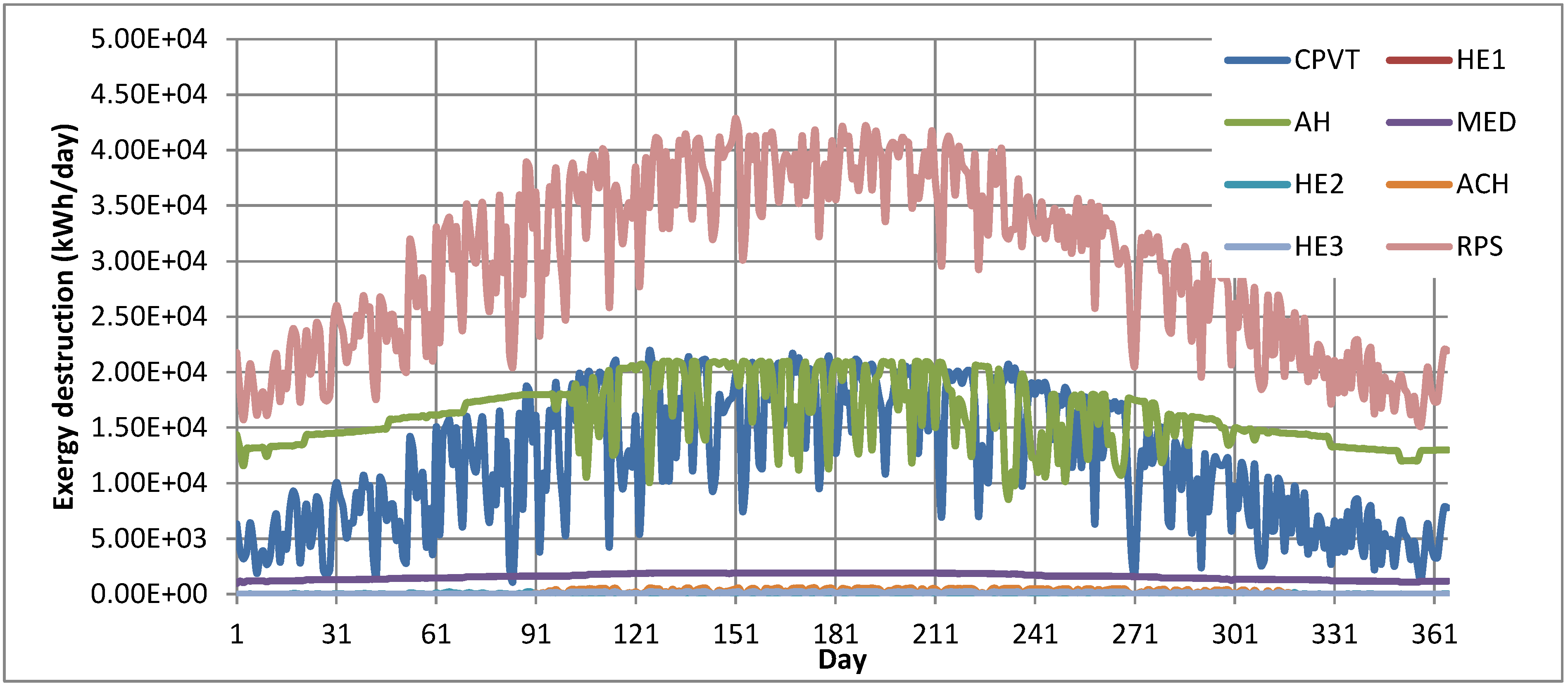
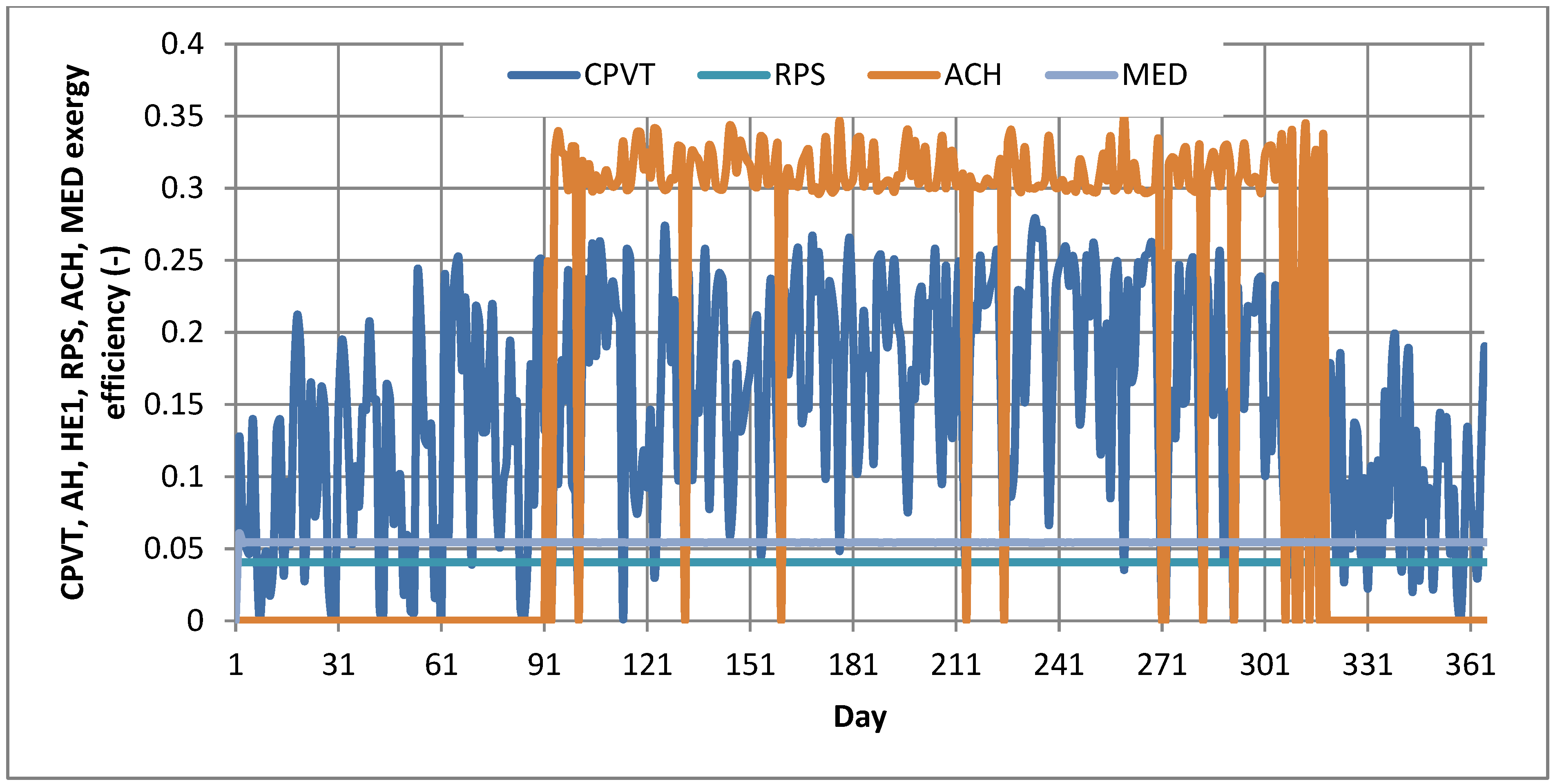
4.1. Exergy Analysis


4.2. Exergoenviromental and Economic Optimizations

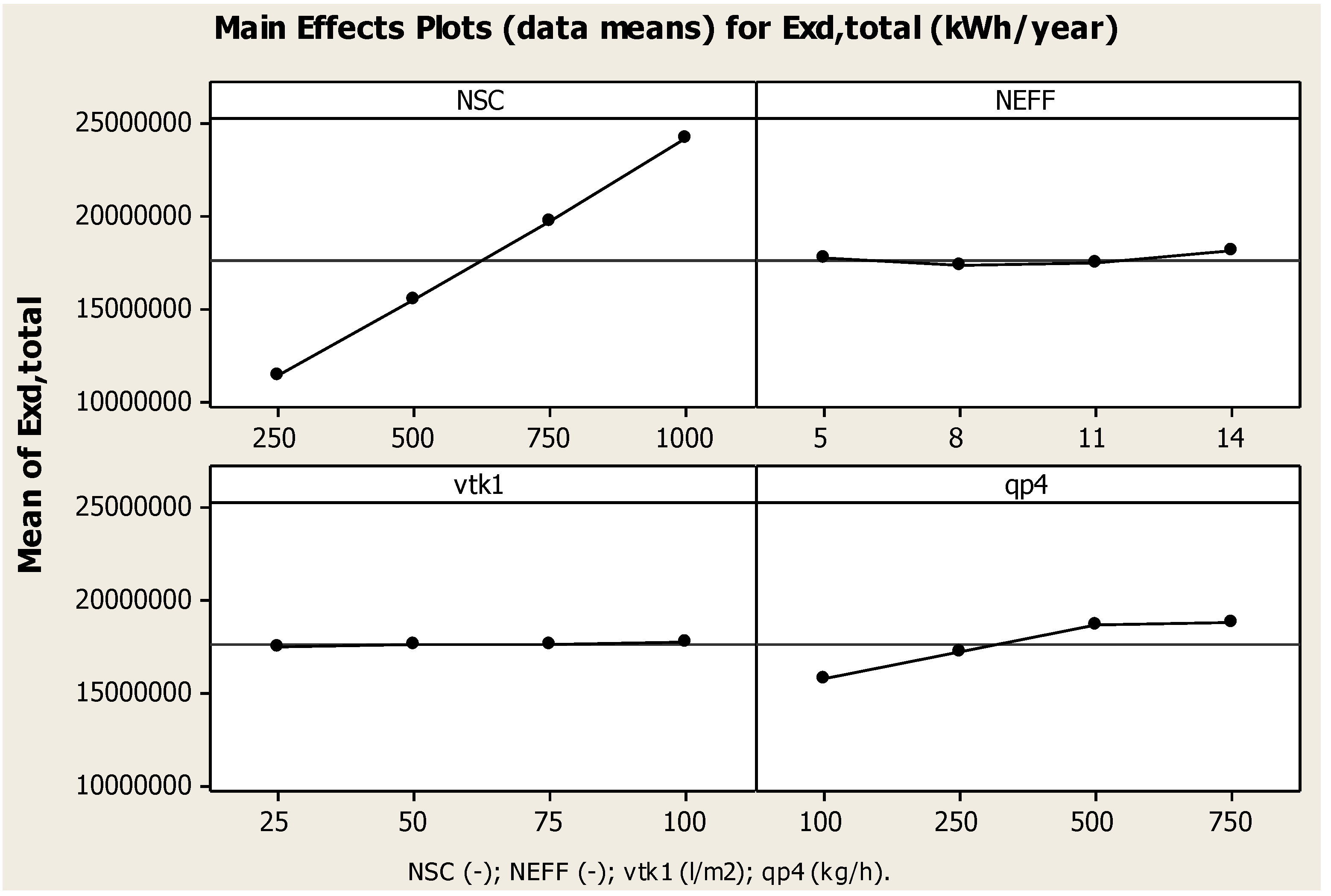
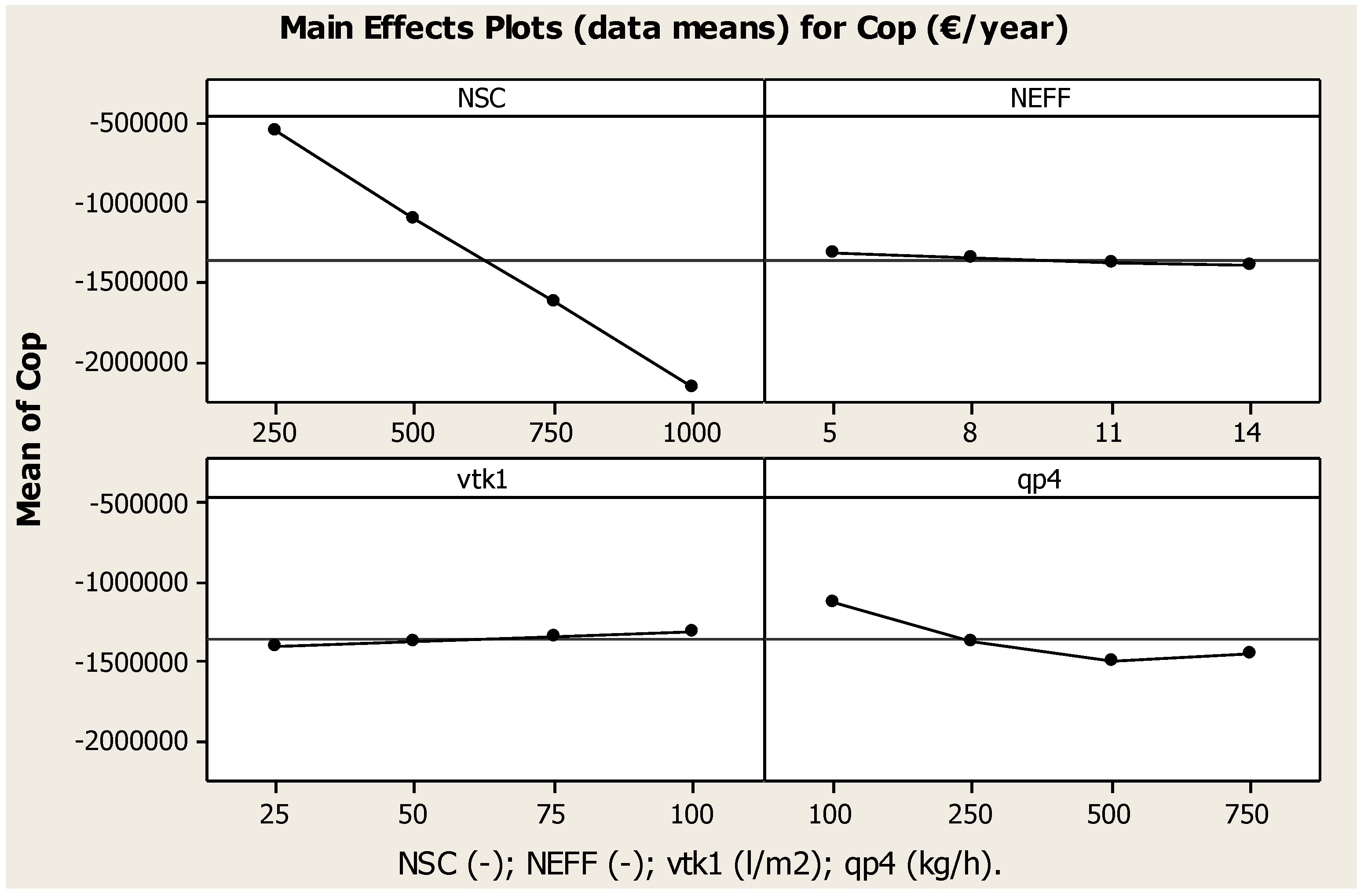
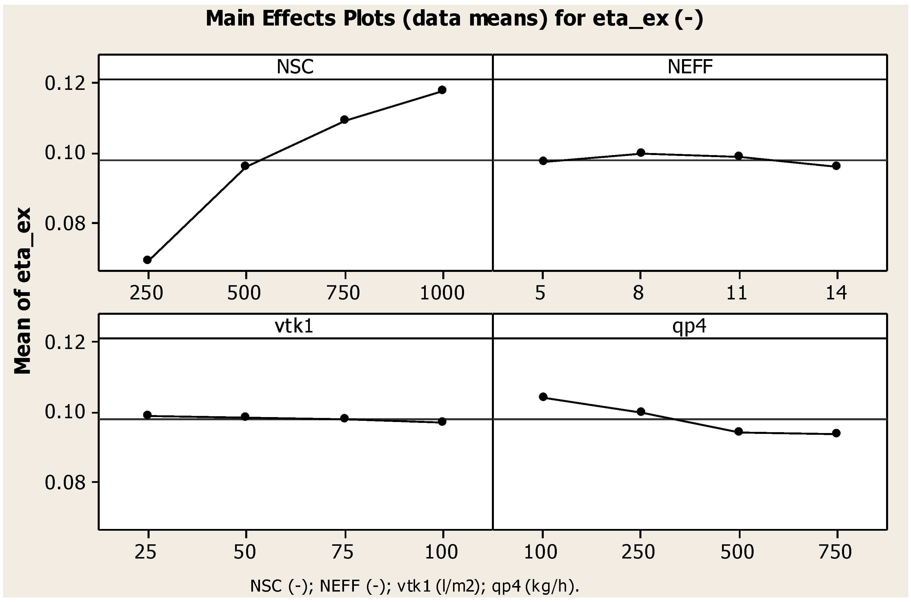
| Variable | Unit | Level 1 | Level 2 | Level 3 | Level 4 |
|---|---|---|---|---|---|
| NSC | (-) | 250 | 500 | 750 | 1000 |
| NEFF | (-) | 5 | 8 | 11 | 14 |
| vTK1 | L/m2 | 25 | 50 | 75 | 100 |
| qp4 | kg/h | 100 | 250 | 500 | 750 |
4.2.1. DoE: Main Effects Plots


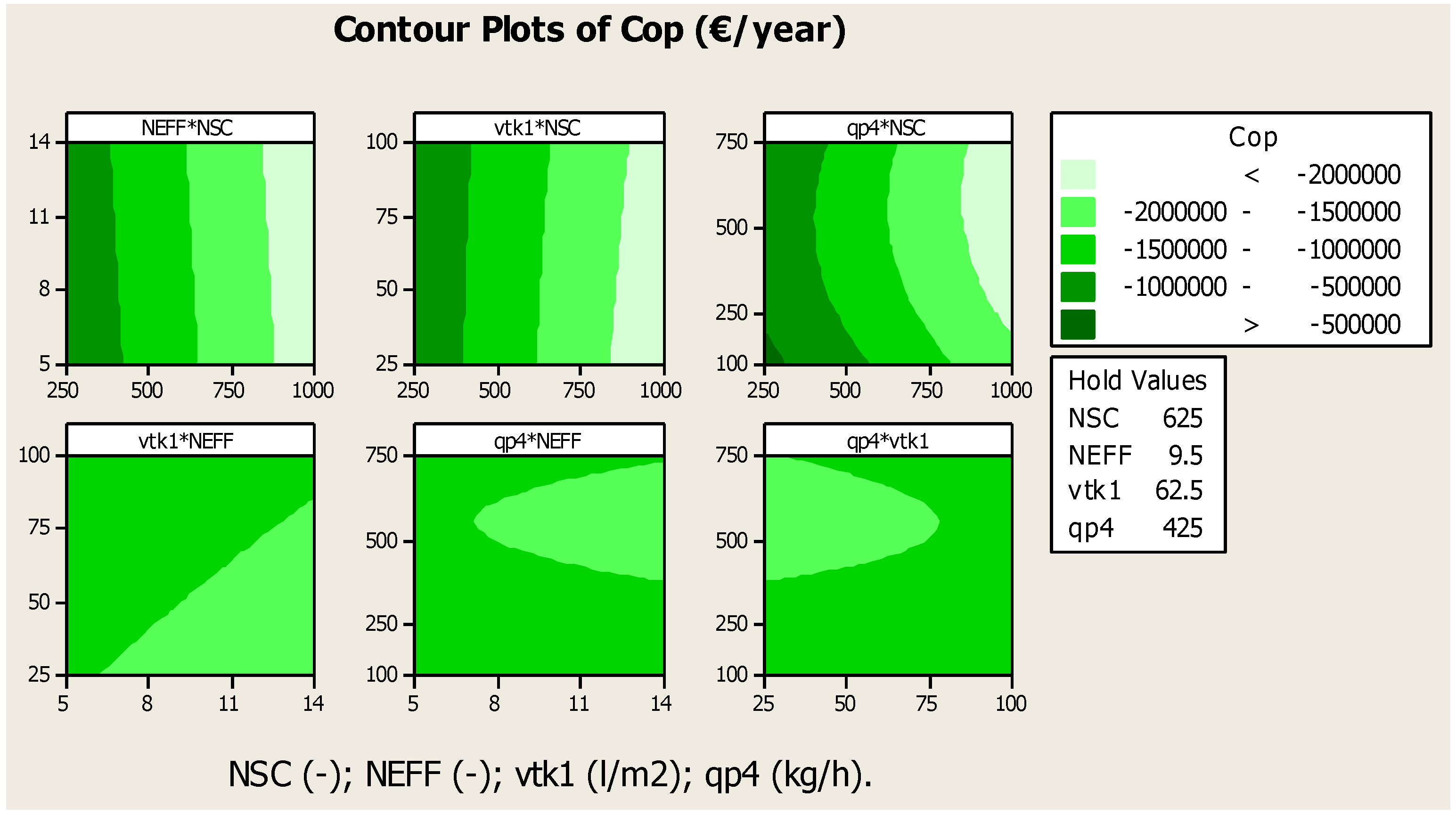
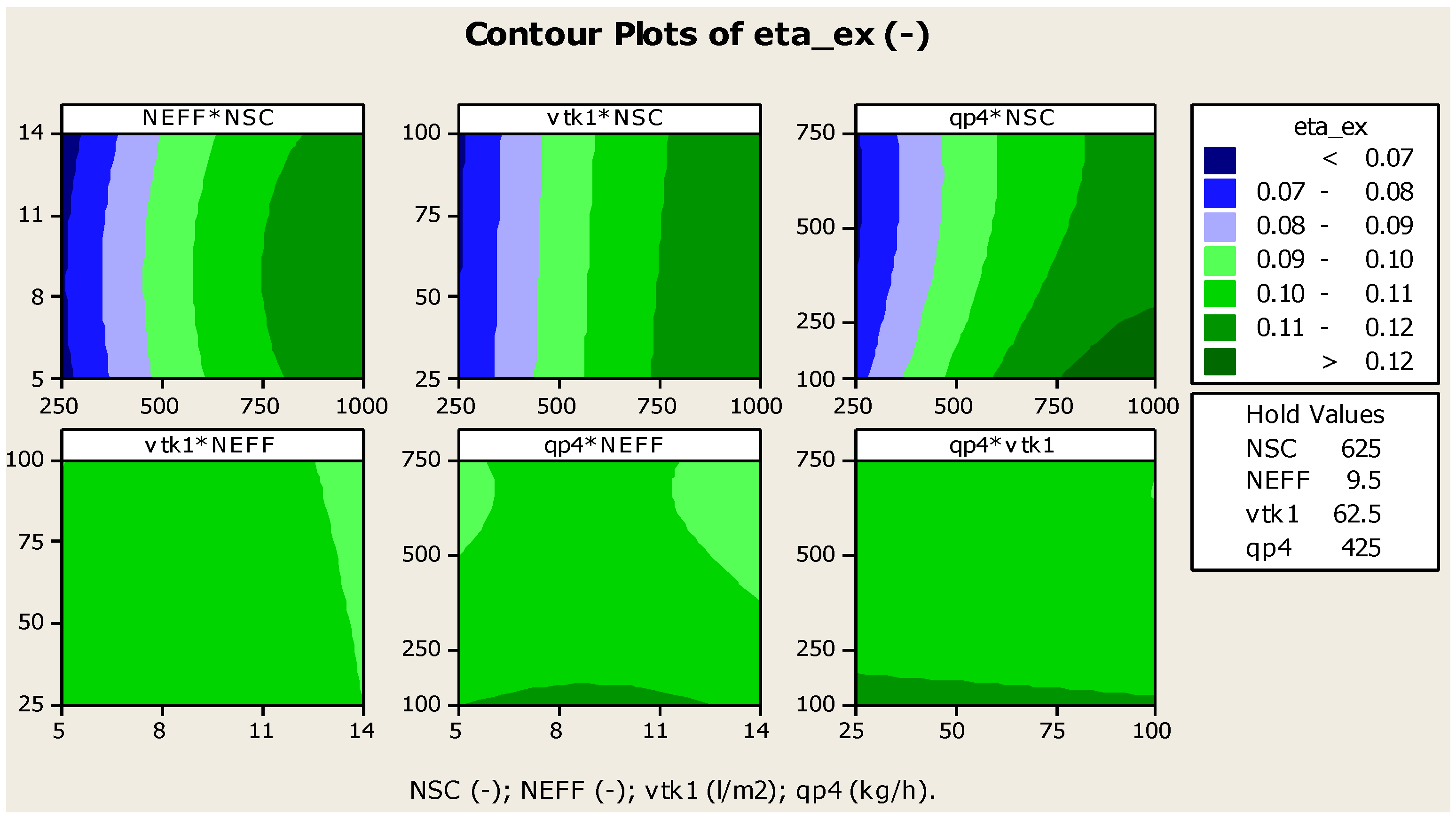
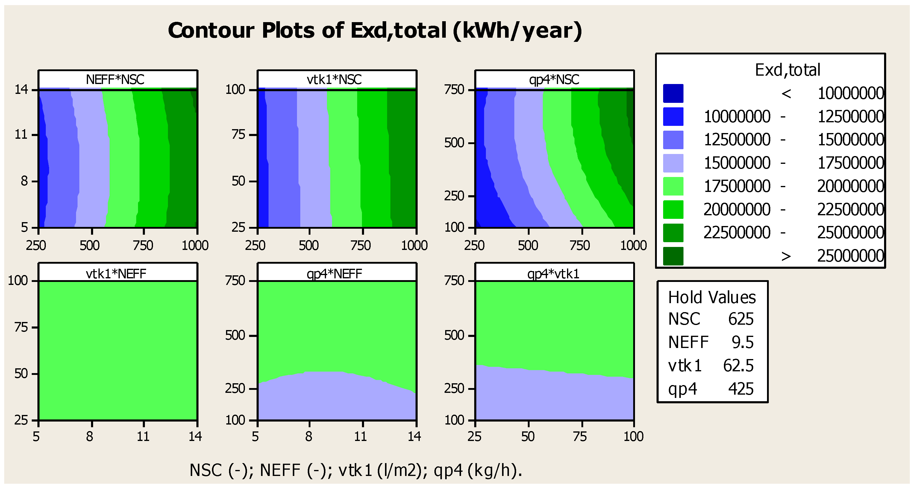
4.2.2. DoE: Contour Plots of the Optimal Response Surface


4.2.3. DoE: Optimization
| OFs | Design variables | Optimal | Initial | |||||||
|---|---|---|---|---|---|---|---|---|---|---|
| Goal | NSC | NEFF | vTK1 | qp4 | Value | Unit | OFs | Value | Unit | |
| - | - | L·m−2 | kg·h−1 | |||||||
| PI | Max. | 760 | 14 | 25 | 475 | 3.43 | - | PI | 2.64 | - |
| Cop | Min. | 1000 | 14 | 25 | 620 | −2480 | k€ | Cop | −541 | k€ |
| ηex | Max. | 1000 | 9 | 25 | 100 | 12.80 | % | ηex | 7.20 | % |
| Exd,total | Min. | 250 | 9 | 25 | 100 | 9.46 | GWh/y | Exd,total | 10.9 | GWh/y |
5. Conclusions
Author Contributions
Nomenclature
Area (m2) | |
Annuity Factor (years) | |
Incomes from trading of CO2 emission certificates (€/year) | |
Specific heat (kJ/kg K) | |
Unit economic value for the CO2 emission saving (€/kgCO2) | |
Annual operating cost (€/year) | |
Specific heat at constant pressure (kJ/kg K) | |
Electric energy (kWh) | |
Electric power (kW) | |
Specific exergy (kJ/kg) | |
Exergy flow (kW) | |
Chemical exergy flow rate (kW) | |
Overall destroyed exergy Objective Function (kWh/year) | |
Emission factor (kg CO2/kWh) | |
Public funding (€/year) | |
Specific enthalpy (kJ/kg) | |
Total radiation (kW/m2) | |
Total capital cost (€) | |
Annual total capital cost (€/year) | |
Mass flow rate (kg/s) | |
Distillated water mass flow rate (kg/s) | |
Molar weight (kg/kmol) | |
Molar flow of fresh water (kmol/s) | |
Number of MED effects collectors (-) | |
Net Present Value (€) | |
Number of solar collectors (-) | |
Pressure (kPa) | |
Daily exergy product (kWh/day) | |
Profit Index Objective Function (-) | |
Thermal energy (kWh) | |
Thermal flow rate (kW) | |
P4 flow rate/ NSC(kg/h) | |
Universal constant of gases (kJ/kmol·K) | |
Specific entropy (kJ/kg·K) | |
Temperature (°C) | |
Temperature (K) | |
Specific volume (m3/kg) | |
TK1 volume per SC surface area (L/m2) | |
| X | Molar concentration of salts in the seawater (ppm) |
Electrical power CPVT (kW) | |
Electric power used by the MED (kW) |
Abbreviations
| ACH | Absorption Chiller |
| AH | Auxiliary Heater |
| BOP | Balance of Plant |
| CHW | Chilled Water |
| CPVT | Concentrating Photovoltaic-Thermal Collector |
| COP | Coefficient of Performance |
| CW | Cooling Water |
| D | Diverter |
| DoE | Design of Experiment |
| DHW | Domestic Hot Water |
| DW | Desalted water |
| HE | Heat exchanger |
| HF | Hot fluid |
| HW | Hot water |
| M | Mixer |
| MED | Multiple-Effect Distillation |
| MSF | Multi-Stage Flash |
| P | Pump |
| PVT | Photovoltaic-Thermal collectors |
| RO | Reverse Osmosis |
| RPS | Renewable Polygeneration System |
| SCF | Solar Collector Fluid |
| SHC | Solar Heating and Cooling |
| SW | Seawater |
| TK | Tank |
Greek Symbols
Dissociation factor (-) | |
Theoretical minimum work of separation (kJ/kmol) | |
Temperature (K) | |
Efficiency (-) | |
Exergy efficiency (-) |
Subscripts
Ambient | |
Auxiliary | |
Auxiliary Heater | |
Brine | |
Biomass | |
Chemical | |
Condensing | |
Concentrating Photovoltaic-Thermal Collector | |
Destroyed | |
Distillate produced by flash at brine inlet at i-th effect | |
Domestic Hot Water | |
Distillate by evaporation at i-th effect | |
Electrical | |
Exergy | |
Seawater in input to the plant | |
Related to the fresh water produced | |
Heating | |
i-th time-step | |
Multi-Effect Distillation | |
Natural gas | |
Physics | |
Salts | |
Sun | |
Traditional | |
Total |
Conflicts of Interest
References
- Agency, I.-I.E. (Ed.) World Energy Outlook 2013; OECD/IEA: Paris, France, 2013.
- IEA. Current Research Projects (Tasks). Available online: http://www.iea-shc.org/tasks-current (accessed on 27 January 2015).
- Sarbu, I.; Sebarchievici, C. Review of solar refrigeration and cooling systems. Energy Build. 2013, 67, 286–297. [Google Scholar] [CrossRef]
- Ullah, K.R.; Saidur, R.; Ping, H.W.; Akikur, R.K.; Shuvo, N.H. A review of solar thermal refrigeration and cooling methods. Renew. Sustain. Energy Rev. 2013, 24, 499–513. [Google Scholar] [CrossRef]
- Zhai, X.Q.; Qu, M.; Wang, R.Z. A review for research and new design options of solar absorption cooling systems. Renew. Sustain. Energy Rev. 2011, 15, 4416–4423. [Google Scholar] [CrossRef]
- Angrisani, G.R.C.; Sasso, M.; Tariello, F. Assessment of energy, environmental and economic performance of a solar desiccant cooling system with different collector types. Energies 2014, 7, 6741–6764. [Google Scholar]
- Calise, F.; Palombo, A.; Vanoli, L. Design and dynamic simulation of a novel solar trigeneration system based on photovoltaic/thermal collectors. Energy Convers. Manag. 2011, 60, 214–225. [Google Scholar] [CrossRef]
- Chow, T.T. A review on photovoltaic/thermal hybrid solar technology. Appl. Energy 2010, 87, 365–379. [Google Scholar] [CrossRef]
- Zondag, H.A. Flat-plate PV-Thermal collectors and systems: A review. Renew. Sustain. Energy Rev. 2008, 12, 891–895. [Google Scholar] [CrossRef]
- Mittelman, G.; Kribus, A.; Dayan, A. Solar cooling with concentrating photovoltaic/thermal (CPVT) systems. Energy Convers. Manag. 2007, 48, 2481–2490. [Google Scholar] [CrossRef]
- Ibrahim, A.; Othman, M.; Ruslan, M.H.; Mat, S.; Sopian, K. Recent advances in flat plate photovoltaic/thermal (PV/T) solar collectors. Renew. Sustain. Energy Rev. 2011, 15, 352–365. [Google Scholar] [CrossRef]
- Nishioka, K.; Takamoto, T.; Agui, T.; Kaneiwa, M.; Uraoka, Y.; Fuyuki, T. Annual output estimation of concentrator photovoltaic systems using high-efficiency InGaP/InGaAs/Ge triple-junction solar cells based on experimental solar cell’s characteristics and field-test meteorological data. Solar Energy Mater. Sol. Cells 2006, 90, 57–67. [Google Scholar] [CrossRef]
- Desalination.com. What Technologies Are Used? 2012. Available online: http://www.desalination.com/market/technologies (accessed on 18 June 2013).
- Tokui, Y.; Moriguchi, H.; Nishi, Y. Comprehensive environmental assessment of seawater desalination plants: Multistage flash distillation and reverse osmosis membrane types in Saudi Arabia. Desalination 2014, 351, 145–150. [Google Scholar] [CrossRef]
- Cardona, E.; Piacentino, A. Optimal design of cogeneration plants for seawater desalination. Desalination 2004, 166, 411–426. [Google Scholar] [CrossRef]
- Ibrahim, S.; Al-Mutaz, A.M.A.-N. Characteristics of dual purpose MSF desalination plants. Desalination 2004, 166, 287–294. [Google Scholar] [CrossRef]
- Cardona, E.; Piacentino, A.; Marchese, F. Performance evaluation of CHP hybrid seawater desalination plants. Desalination 2007, 205, 1–14. [Google Scholar] [CrossRef]
- Osman, A.; Hamed, H.A.A.-O. Prospects of operation of MSF desalination plants at high TBT and low antiscalant dosing rate. Desalination 2010, 256, 181–189. [Google Scholar] [CrossRef]
- Esfahani, I.J.; Ataei, A.; Shetty, K.V.; Oh, T.; Park, J.H.; Yoo, C. Modeling and genetic algorithm-based multi-objective optimization of the MED-TVC desalination system. Desalination 2012, 292, 87–104. [Google Scholar] [CrossRef]
- Palenzuela, P.; Hassan, A.S.; Zaragoza, G.; Alarcón-Padilla, D.-C. Steady state model for multi-effect distillation case study: Plataforma Solar de Almería MED pilot plant. Desalination 2014, 337, 31–42. [Google Scholar] [CrossRef]
- Calise, F.; d’Accadia, M.D.; Piacentino, A. A novel solar trigeneration system integrating PVT (photovoltaic/thermal collectors) and SW (seawater) desalination: Dynamic simulation and economic assessment. Energy 2014, 67, 129–148. [Google Scholar] [CrossRef]
- Calise, F.; Cipollina, A.; d’Accadia, M.D.; Piacentino, A. A novel renewable polygeneration system for a small mediterranean volcanic island for the combined production of energy and water: Dynamic simulation and economic assessment. Appl. Energy 2014, 135, 675–693. [Google Scholar] [CrossRef]
- Koroneos, C.; Tsarouhis, M. Exergy analysis and life cycle assessment of solar heating and cooling systems in the building environment. J. Clean. Prod. 2012, 32, 52–60. [Google Scholar] [CrossRef]
- Onan, C.; Ozkan, D.B.; Erdem, S. Exergy analysis of a solar assisted absorption cooling system on an hourly basis in villa applications. Energy 2010, 35, 5277–5285. [Google Scholar] [CrossRef]
- Calise, F.; Palombo, A.; Vanoli, L. A finite-volume model of a parabolic trough photovoltaic/thermal collector: Energetic and exergy analyses. Energy 2012, 46, 283–294. [Google Scholar] [CrossRef]
- El-Nashar, M.A.; Al-Baghdadi, A.A. Exergy losses in a multiple-effect stack seawater desalination plant. Desalination 1998, 116, 11–24. [Google Scholar] [CrossRef]
- Nafey, A.S.; Fath, H.E.S.; Mabrouk, A.A. Exergy and thermoeconomic evaluation of MSF process using a new visual package. Desalination 2006, 201, 224–240. [Google Scholar] [CrossRef]
- Sharaf, M.A.; Nafey, A.S.; García-Rodríguez, L. Exergy and thermo-economic analyses of a combined solar organic cycle with multi effect distillation (MED) desalination process. Desalination 2011, 272, 135–147. [Google Scholar] [CrossRef]
- Sharqawy, M.H.; Lienhard, V.J.H.; Zubair, S.M. On exergy calculations of seawater with applications in desalination systems. Int. J. Therm. Sci. 2011, 50, 187–196. [Google Scholar] [CrossRef]
- Al-Weshahi, M.A.; Anderson, A.; Tian, G. Exergy efficiency enhancement of MSF desalination by heat recovery from hot distillate water stages. Appl. Therm. Eng. 2013, 53, 226–233. [Google Scholar] [CrossRef]
- Nematollahi, F.; Rahimi, A.; Gheinani, T.T. Experimental and theoretical energy and exergy analysis for a solar desalination system. Desalination 2013, 317, 23–31. [Google Scholar] [CrossRef]
- Jin, C.-Z.; Chou, Q.L.; Jiao, D.S.; Shu, P.C. Vapour compression flash seawater desalination system and its exergy analysis. Desalination 2014, 353, 75–83. [Google Scholar] [CrossRef]
- Uche, J.; Serra, L.; Valero, A. Thermoeconomic optimization of a dual-purpose power and desalination plant. Desalination 2001, 136, 147–158. [Google Scholar] [CrossRef]
- Fiorini, P.; Sciubba, E. Modular simulation and thermoeconomic analysis of a multi-effect distillation desalination plant. Energy 2007, 32, 459–466. [Google Scholar] [CrossRef]
- Mabrouk, A.A.; Nafey, A.S.; Fath, H.E.S. Thermoeconomic analysis of some existing desalination processes. Desalination 2007, 205, 354–373. [Google Scholar] [CrossRef]
- Sayyaadi, H.; Saffari, A. Thermoeconomic optimization of multi effect distillation desalination systems. Appl. Energy 2010, 87, 1122–1133. [Google Scholar]
- Sayyaadi, H.; Saffari, A.; Mahmoodian, A. Various approaches in optimization of multi effects distillation desalination systems using a hybrid meta-heuristic optimization tool. Desalination 2010, 254, 138–148. [Google Scholar] [CrossRef]
- Hosseini, S.R.; Amidpour, M.; Behbahaninia, A. Thermoeconomic analysis with reliability consideration of a combined power and multi stage flash desalination plant. Desalination 2011, 278, 424–433. [Google Scholar] [CrossRef]
- Li, M.; Ji, X.; Li, G.L.; Yang, Z.M.; Wei, S.X.; Wang, L.L. Performance investigation and optimization of the Trough Concentrating Photovoltaic/Thermal system. Sol. Energy 2011, 85, 1028–1034. [Google Scholar] [CrossRef]
- El-Emam, R.S.; Dincer, I. Thermodynamic and thermoeconomic analyses of seawater reverse osmosis desalination plant with energy recovery. Energy 2014, 64, 154–163. [Google Scholar] [CrossRef]
- Calise, F.; d’Accadia, M.D.; Vanoli, L. Thermoeconomic optimization of Solar Heating and Cooling systems. Energy Convers. Manag. 2011, 52, 1562–1573. [Google Scholar] [CrossRef]
- Hang, Y.; Du, L.; Qu, M.; Peeta, S. Multi-objective optimization of integrated solar absorption cooling and heating systems for medium-sized office buildings. Renew. Energy 2013, 52, 67–78. [Google Scholar]
- Zou, Z.; Guan, Z.; Gurgenci, H. Optimization design of solar enhanced natural draft dry cooling tower. Energy Convers. Manag. 2013, 76, 945–955. [Google Scholar] [CrossRef]
- Wang, M.; Wang, J.; Zhao, P.; Dai, Y. Multi-objective optimization of a combined cooling, heating and power system driven by solar energy. Energy Convers. Manag. 2015, 89, 289–297. [Google Scholar] [CrossRef]
- Calise, F. Thermoeconomic analysis and optimization of high efficiency solar heating and cooling systems for different Italian school buildings and climates. Energy Build. 2010, 42, 992–1003. [Google Scholar] [CrossRef]
- Sharaf, O.Z.; Orhan, M.F. Concentrated photovoltaic thermal (CPVT) solar collector systems: Part II—Implemented systems, performance assessment, and future directions. Renew. Sustain. Energy Rev. 2014. [Google Scholar] [CrossRef]
- Calise, F.; d’Accadia, M.D.; Vanoli, L. Design and dynamic simulation of a novel solar trigeneration system based on hybrid photovoltaic/thermal collectors (PVT). Energy Convers. Manag. 2012, 60, 214–225. [Google Scholar] [CrossRef]
- Evola, G.; Marletta, L. Exergy and thermoeconomic optimization of a water-cooled glazed hybrid photovoltaic/thermal (PVT) collector. Sol. Energy 2014, 107, 12–25. [Google Scholar] [CrossRef]
- Khoshgoftar Manesh, M.H.; Ghalami, H.; Amidpour, M.; Hamedi, M.H. Optimal coupling of site utility steam network with MED-RO desalination through total site analysis and exergoeconomic optimization. Desalination 2013, 316, 42–52. [Google Scholar] [CrossRef]
- Walpole, R.E.; Myers, R.H.; Myers, S.L.; Ye, K.E. Probability and Statistics for Engineers and Scientists, 9th ed.; Pearson: Upper Saddle River, NJ, USA, 1993. [Google Scholar]
- Calise, F.; Palombo, A.; Vanoli, L. Maximization of primary energy savings of solar heating and cooling systems by transient simulations and computer design of experiments. Appl. Energy 2010, 87, 524–540. [Google Scholar] [CrossRef]
- Rosen, M.A.; Dincer, I. Effect of varying dead-state properties on energy and exergy analyses of thermal systems. Int. J. Therm. Sci. 2004, 43, 121–133. [Google Scholar] [CrossRef]
- Kotas, T.J. The Exergy Method of Thermal Plant Analysis; Paragon Publishing: Wiltshire, UK, 1995. [Google Scholar]
- Torío, H.; Angelotti, A.; Schmidt, D. Exergy analysis of renewable energy-based climatisation systems for buildings: A critical view. Energy Build. 2009, 41, 248–271. [Google Scholar] [CrossRef]
- Ajam, H.; Farahat, S.; Saehaddi, F. Exergy Optimization of solar air heaters and comparison with energy analysis. Int. J. Thermodyn. 2005, 8, 183–190. [Google Scholar]
- Song, G.; Shen, L.; Xiao, J. Estimating specific chemical exergy of biomass from basic analysis data. Ind. Eng. Chem. Re. 2011, 50, 9758–9766. [Google Scholar] [CrossRef]
- Spiegler, K.S.; El-Sayed, Y.M. The energetics of desalination processes. Desalination 2001, 134, 109–128. [Google Scholar] [CrossRef]
© 2015 by the authors; licensee MDPI, Basel, Switzerland. This article is an open access article distributed under the terms and conditions of the Creative Commons Attribution license (http://creativecommons.org/licenses/by/4.0/).
Share and Cite
Calise, F.; D'Accadia, M.D.; Piacentino, A.; Vicidomini, M. Thermoeconomic Optimization of a Renewable Polygeneration System Serving a Small Isolated Community. Energies 2015, 8, 995-1024. https://doi.org/10.3390/en8020995
Calise F, D'Accadia MD, Piacentino A, Vicidomini M. Thermoeconomic Optimization of a Renewable Polygeneration System Serving a Small Isolated Community. Energies. 2015; 8(2):995-1024. https://doi.org/10.3390/en8020995
Chicago/Turabian StyleCalise, Francesco, Massimo Dentice D'Accadia, Antonio Piacentino, and Maria Vicidomini. 2015. "Thermoeconomic Optimization of a Renewable Polygeneration System Serving a Small Isolated Community" Energies 8, no. 2: 995-1024. https://doi.org/10.3390/en8020995