Educational Project for the Teaching of Control of Electric Traction Drives

Abstract

Electric vehicles constitute a multidisciplinary subject that involves disciplines such as automotive, mechanical, electrical and control engineering. Due to this multidisciplinary technical nature, practical teaching methodologies are of special relevance. Paradoxically, in the past, the training of engineers specializing in this area has lacked the practical component represented by field tests, due to the difficulty of accessing real systems. This paper presents an educational project specifically designed for the teaching and training of engineering students with different backgrounds and experience. The teaching methodology focuses on the topology of electric traction drives and their control. It includes two stages, a simulation computer model and a scaled laboratory workbench that comprises a traction electrical drive coupled to a vehicle emulator. With this equipment, the effectiveness of different traction control strategies can be analyzed from the point of view of energy efficiency, robustness, easiness of implementation and acoustic noise.

1. Introduction

In the last decade, electric vehicles (EVs) have experienced a continuous and noteworthy improvement in their performance. Nowadays, electric automobiles have the potential to become a feasible alternative to conventional internal combustion vehicles, especially in urban environments.

As EV technology develops, better performance is expected, and therefore more specific power electronics converters and more sophisticated control strategies are imposed on these systems. Since this technological demand must be fulfilled within the educational community, it is the responsibility of niversities to teach and train future engineers on this matter, although it is also very desirable that the industry collaborates with this process for mutual benefit.

Mainly due to the difficulty in accessing this kind of drive in a real vehicle, studies on electric traction technologies are typically based on theoretical lessons, while practical application of the fundamental concepts is required for a realistic active learning experience [1]. In most educational centers, this practical experience has been carried out only by means of computer simulation models [2,3], without the benefits brought by the actual machines and by the performance of field tests in the laboratory [4].

To overcome the limitations of the abovementioned methodologies, a laboratory-based platform is proposed in this paper. Similar works have already been published for other engineering applications, such as programmable and configurable embedded systems [5], electrical drives control [6,7] and wind generators control [8,9]. The work presented in [5] shows how these kind of project-based learning methods may improve teaching in multidisciplinary systems, while [8,9] are examples of teaching methodologies combining simulation and a laboratory test bench.

This paper describes a complete system dedicated to the teaching and training of engineering students on the control of electric traction drives. The work has been developed within the Polytechnic University of Madrid in collaboration with CIEMAT, a public research center focused on the transfer of knowledge between researchers and industry.

2. Teaching Objectives and General Approach

The main objectives of the proposed educational project are to complement the theoretical lessons regarding traction drives and their control, to motivate the students’ interest in topics covered in those lectures and to introduce them to the design process of control strategies for EVs. In terms of technology, the project exposes students to devices currently used in EVs, such as batteries, power converters and traction machines, which they will meet in the industry. Besides, the course also covers some design tools for new control strategies.

The educational project targets Master’s degree students in the field of mechanical, electrical or electronic engineering. It was designed as part of an already existing 40-h course in EVs. The proposed teaching methodology comprises two different learning levels:

(1)

A basic level, consisting in a computer simulator based on electrical models of the different components of the drive: energy storage system, power electronics converters, electrical machine and the vehicle itself. A first learning stage includes a series of exercises designed to introduce the students to the system. In a second stage, the students develop their own control strategies based on simulations.

(2)

An advanced level, consisting in a reduced scale emulator of the powertrain of an electric vehicle. This emulator is a laboratory workbench that includes a DC voltage source, two power electronics inverters, and two electric motors, one to emulate the inertia and motion resistances of the vehicle and the other the traction machine itself. Using this equipment, and always assisted by a supervisor, the students can test the control strategies developed in the previous stage.

During the development of this system and its associated training methodology, especial focus was put on three remarkable and differentiating aspects of EV teaching:

(1)

Electric vehicles are a multidisciplinary subject. Therefore, students with different backgrounds (from mechanical to electronic engineering) had to be taken into account.

(2)

A smooth learning curve was desirable, which meant carefully planning the progression of the different exercises within the course.

(3)

The course had to be as practical as possible. In this sense, it was not enough to show the students a laboratory platform. Higher interaction with the test bench was desired.

Despite its educational focus, the proposed computer and laboratory platforms were designed for both research and teaching purposes. In this sense, the system is also suitable for testing new control strategies in electrical traction drive research.

3. Technology Overview: Powertrain of a Battery Electric Vehicle

The powertrain of a vehicle includes all the necessary components used to transform stored energy into kinetic energy for propulsion purposes. In a rechargeable electric automobile, this always includes the on-board energy storage system (usually batteries, but sometimes a combination of batteries and ultracapacitors [10]), one or more bidirectional power electronics converters (usually two, one DC/DC converter and one inverter or DC/AC converter), and one or more rotatory electrical machines [11,12]. Other elements such as differentials or additional gears are also present depending on the powertrain topology. 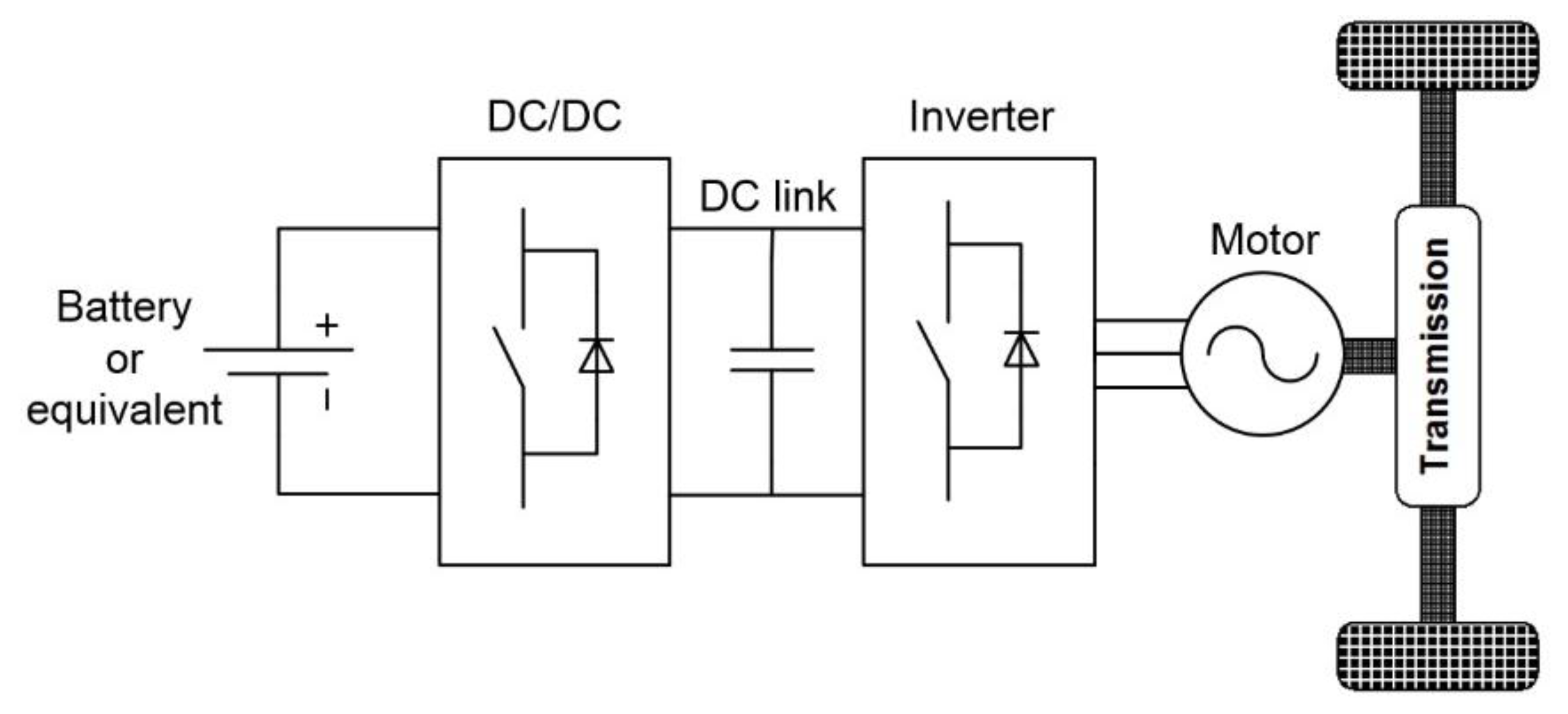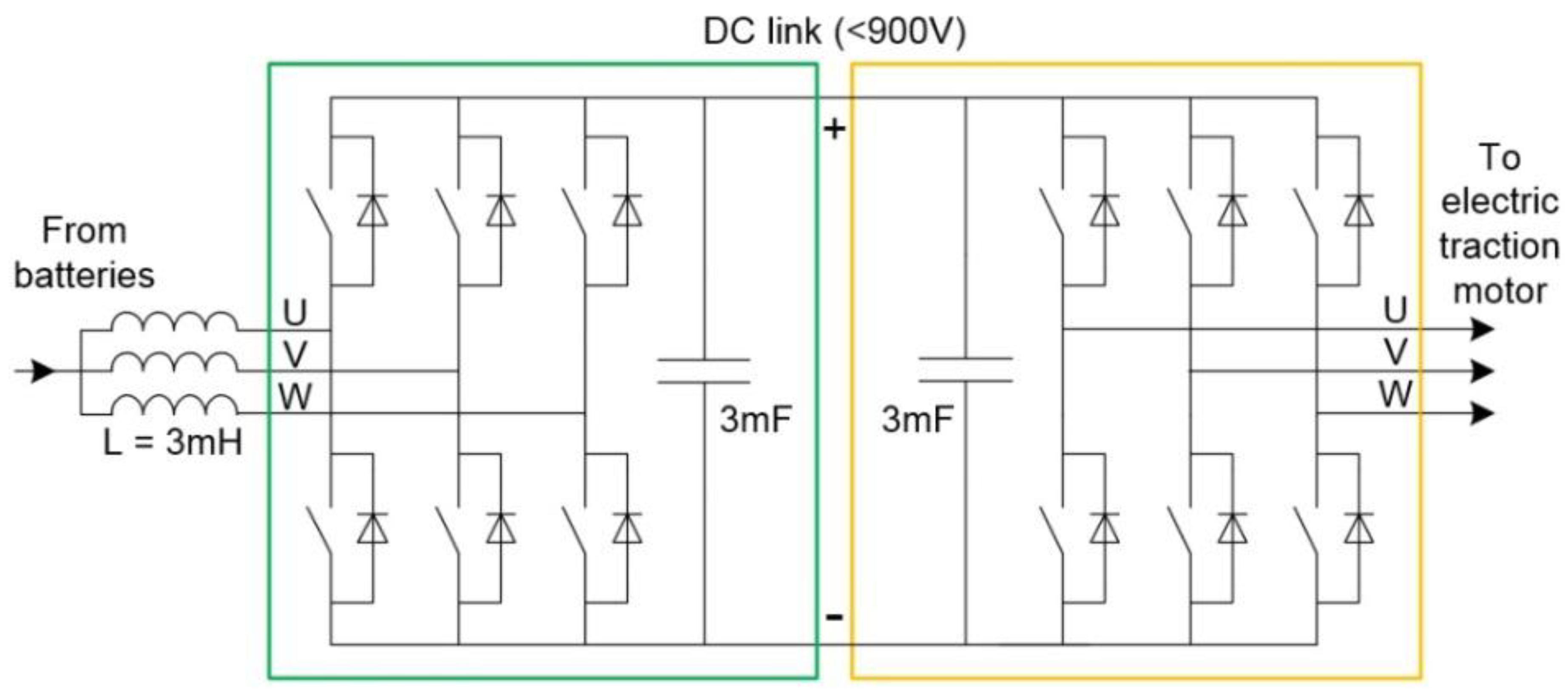Figure 1 shows one of the most common powertrain topologies found in battery EVs, which is the one studied in this work.

Figure 1. Powertrain topology of a battery electric vehicle used in this paper.

Figure 1. Powertrain topology of a battery electric vehicle used in this paper.

Given the above topology, the control strategy is as follows:

(1)

The DC/AC converter works as a voltage source inverter. By means of this converter, both machine flux and machine torque are controlled, either directly or indirectly. The power needed by the motor is instantaneously drawn from the DC link, unless the drive is performing a regenerative braking, in which case power will be delivered to the DC link.

(2)

The DC/DC converter works as a conventional buck-boost converter. It dynamically adapts the battery voltage to the DC link voltage while supplying the power needed by the inverter. In traction drives, the DC voltage is usually higher than the battery voltage. The DC voltage may be constant or not, depending on the switching strategy selected for the inverter.

In this work, this same topology was chosen for the educational platform because it is one of the most extensively used traction technologies and because it is highly suitable for the implementation of advanced control features.

4. Simulation-Based Teaching Platform

4.1. Simulation Model

The first training tool developed within this educational project is a computer model in Matlab Simulink^®. This model represents the powertrain of a battery electric vehicle and includes all the elements already mentioned. The algorithms and mathematical models employed in this simulation model are especially robust and simple, so that they are accessible to the students. Figure 2 shows a screenshot of the root level of the model.

Figure 2. Simulation model (root level). Arrows represent either Simulink signals or SimPowerSystems connections.

Figure 2. Simulation model (root level). Arrows represent either Simulink signals or SimPowerSystems connections.

The model has two main parts, as indicated in Figure 2. The energy storage part on the left includes the battery, the DC/DC converter and its corresponding control. This part can be replaced by an ideal DC voltage source in order to simplify the model at the beginning of the learning process. The motor part in the right includes the inverter, the traction machine, the control system and the vehicle itself, modeled as an equivalent load in terms of mass, inertia and motion resistances.

The following paragraphs describe the mathematical models implemented within each one of the blocks in Figure 2, from left to right.

4.1.1. Battery Stack

The battery model is a modification of the generic model provided by Mathworks in the SimPowerSystems library of Simulink^® [13], which was first proposed in [14]. That model is actually a simplification of the highly accepted model described in [15], which in turn is based on an equivalent electrical circuit. The advantages of the model used in this work are its easiness-to-use, its accuracy given its simplicity, and its dynamic behavior. Namely, the battery is modeled as depicted in Figure 3, the equations being as follows:

$$\mathrm{E}=\text{f}\left(\text{SoC}\right)={\mathrm{E}}_0-\text{K}\times {\text{Q}}_{\text{MAX}}\times \left(\frac{100}{\text{SoC}}-1\right)-\text{A}\times {\text{e}}^{-\text{B}\times {\text{Q}}_{\text{MAX}}\times \left(1-\raisebox{1ex}{$\text{SoC}$}\!\left/ \!\raisebox{-1ex}{$100$}\right.\right)}$$

(1)

$${\text{R}}_{\text{POL},\text{discharge}}=\text{f}\left(\text{SoC}\right)=\text{K}\times \frac{100}{\text{SoC}}$$

(2)

$${\text{R}}_{\text{POL},\text{charge}}=\text{f}\left(\text{SoC}\right)=\text{K}\times \frac{1}{1.1-\frac{\text{SoC}}{100}}$$

(3)

where: U: battery instantaneous voltage (V); i: battery current (A), i > 0 when discharging and i < 0 during recharge; SoC: battery state of charge (%); R_SELF: self-discharge resistance (Ω); R_OHM: ohmic internal resistance (Ω); R_POL: polarization internal resistance (Ω); C_POL: polarization capacitor (F); E: open-circuit nonlinear voltage (V); E₀: open-circuit constant voltage (V); K: polarization constant (Ah⁻¹) or polarization resistance constant (Ω); Q_MAX: maximum capacity (Ah); A: exponential voltage (V); B: exponential capacity (Ah⁻¹).

Figure 3. Battery model included in the simulation platform.

Figure 3. Battery model included in the simulation platform.

According to the proposed lithium-ion battery model, the steady-state voltage is:

$$\mathrm{U}=\mathrm{E}-\left({\text{R}}_{\text{OHM}}+{\text{R}}_{\text{POL}}\right)\times \text{i}$$

(4)

The proposed model differs from that in [14] in that it loses generality for the sake of simplicity, since it is only valid for lithium-ion batteries. Besides, the internal resistance is modeled as two different electrical resistances: ohmic resistance (constant) and polarization resistance (variable), the latter being dependent on the SoC. An important advantage of the proposed model lies on its formulation, which is easier to understand from a student point of view given that less variables are involved.

4.1.2. DC/DC Converter and DC Link

The models for the power electronics converters are also based on power semiconductors included in the SimPowerSystems library, namely the “IGBT” and the “diode” blocks [13]. The power devices used in this work are those of the IGBT module “SEMiX71GD12E4s” by Semikron [16]. Both the DC/DC and the DC/AC converters use the same conventional three-phase IGBT bridge with anti-parallel diodes (see Figure 4) [17]. Despite their similar topology, both converters have very different functionality due to the way they are connected to the rest of the system and to how they are controlled. Using the same topology in both converters helps the students to better understand the power electronics involved in this system. The DC/DC converter works as a bidirectional multiphase (interleaved topology) buck-boost converter [18], connecting to the batteries by means of three parallel inductances (3 mH each).

Figure 4. Power electronics topology (simplified scheme).

Figure 4. Power electronics topology (simplified scheme).

Finally, the DC link is composed of a group of capacitors (1100 V, 0.5 mF) connected in parallel. The equivalent total capacitance is 6 mF.

4.1.3. Inverter

The DC/AC converter is modeled the same way as the DC/DC converter. However, in this case the converter works as a conventional three-phase current-controlled voltage source inverter (VSI), as shown in Figure 4 [17,19].

4.1.4. Traction Machine

The electric motor model is suitable for any synchronous machine: permanent magnet synchronous machine (PMSM), synchronous reluctance machine (SRM), or anything in between (such as permanent magnet assisted SRM). The model is based in data extracted from finite element simulations and laboratory tests, and takes saturation, cross coupling, copper and mechanical losses into account. Therefore, only iron losses and 3D effects are neglected. The equations implemented in the model are the following [20] (amplitude-invariant Clarke transformation [21]):

$$\left[\begin{array}{c}{\text{u}}_{\text{d}}\\ {\text{u}}_{\text{q}}\end{array}\right]={\text{R}}_{\text{S}}\times \left[\begin{array}{c}{\text{i}}_{\text{d}}\\ {\text{i}}_{\text{q}}\end{array}\right]+\frac{\text{d}}{\text{dt}}\left[\begin{array}{c}{\mathrm{\lambda }}_{\text{d}}\\ {\mathrm{\lambda }}_{\text{q}}\end{array}\right]+{\mathrm{\omega }}_{\text{elec}}\times \left[\begin{array}{cc}0& -1\\ 1& 0\end{array}\right]\times \left[\begin{array}{c}{\mathrm{\lambda }}_{\text{d}}\\ {\mathrm{\lambda }}_{\text{q}}\end{array}\right]$$

(5)

$${\text{T}}_{\text{em}}=\frac{3}{2}\times \text{p}\times \left({\mathrm{\lambda }}_{\text{d}}\times {\text{i}}_{\text{q}}-{\mathrm{\lambda }}_{\text{q}}\times {\text{i}}_{\text{d}}\right)$$

(6)

$${\text{T}}_{\text{em}}-{\text{T}}_{\text{load}}=\mathrm{J}\times \frac{{\text{dω}}_{\text{mec}}}{\text{dt}}+\text{B}\times {\mathrm{\omega }}_{\text{mec}}$$

(7)

where: u_d, u_q: stator voltages in dq reference frame (V); i_d, i_q: stator currents in dq reference frame (A); R_S: stator winding resistance (Ω); λ_d, λ_q: stator flux linkages in dq reference frame (Wb); ω_elec: rotor electrical speed (rad/s); T_em: electromagnetic torque (Nm); p: pole pairs (-); T_load: load torque (Nm); J: total moment of inertia (kg·m²); ω_mec: rotor mechanical speed (rad/s); B: total friction (Nm/(rad/s)).

The above equations are complemented with two look-up tables (LUTs) that link stator currents to flux linkages, as expressed by Equation (8), where θ_S is the stator-current phasor angle:

$$\begin{gathered} {\mathrm{\lambda }}_{\text{d}}=\text{f}\left({\text{I}}_{\text{S}},{\mathrm{\theta }}_{\text{S}}\right)=\text{g}\left({\text{i}}_{\text{d}},{\text{i}}_{\text{q}}\right) \\ {\mathrm{\lambda }}_{\text{q}}=\text{f}\left({\text{I}}_{\text{S}},{\mathrm{\theta }}_{\text{S}}\right)=\text{g}({\text{i}}_{\text{d}},{\text{i}}_{\text{q}}) \end{gathered}$$

(8)

These LUTs are machine-specific, and are calculated by means of finite element simulations [22]. Figure 5 depicts the LUTs for a 3.3 kW interior PMSM, which is the machine used in the test bench described later in this paper and whose rated values are given in Table 1 (Section 5):

Figure 5. Interior PMSM LUTs relating stator current and flux linkages (simulation results).

Figure 5. Interior PMSM LUTs relating stator current and flux linkages (simulation results).

The torque generated by that same PMSM is shown in Figure 6, along with the corresponding maximum torque per ampere (MTPA) trajectory [20,23].

Figure 6. Interior PMSM torque as a function of stator current and MTPA trajectory (simulation results).

Figure 6. Interior PMSM torque as a function of stator current and MTPA trajectory (simulation results).

4.1.5. Vehicle and Motion Resistances

The vehicle model represents both the inertia of the vehicle and its motion resistances. These include rolling resistance, aerodynamic drag and gradient resistance; the last one being of active nature (may take negative values and contribute to the movement of the vehicle). Transmission losses are also accounted for. The three motion resistances are modeled as follows [24,25,26,27]:

$${\text{F}}_{\text{T}}={\text{F}}_{\text{aero}}+{\text{F}}_{\text{roll}}+{\text{F}}_{\text{grav}}$$

(9)

$${\text{F}}_{\text{aero}}=\frac{1}{2}\times \mathrm{\rho }\times {\text{A}}_{\text{F}}\times {\text{C}}_{\text{D}}\times {(\text{v}-{\text{v}}_{\text{WIND}})}^2\ge 0$$

(10)

$${\text{F}}_{\text{roll}}={\mathrm{\mu }}_{\text{rod}}\times \text{M}\times \text{g}\times \cos (\mathrm{\alpha })>0$$

(11)

$$\text{with} {\mathrm{\mu }}_{\text{roll}}={\mathrm{\mu }}_{\text{roll},0}+{\mathrm{\mu }}_{\text{roll},\text{S}}\times {\text{v}}^{2.5}$$

(12)

$${\text{F}}_{\text{grav}}=\text{M}\times \text{g}\times \text{sin}(\mathrm{\alpha })\gtrless 0$$

(13)

where: F_T: total motion resistance (N); F_aero: aerodynamic resistance (N); F_roll: rolling resistance (N); F_grav: gradient resistance (N); ρ: air mass density (kg/m³); A_F: vehicle frontal area (m²); C_D: vehicle drag coefficient (-); v: vehicle speed (m/s); v_wind: headwind speed (positive in the same direction than the vehicle) (m/s); M: total mass of the vehicle (kg); g: free fall acceleration (m/s²); α: road slope (positive when climbing) (°); µ_roll: rolling friction coefficient (-); µ_roll,0: constant rolling friction coefficient (-); µ_roll,S: incremental rolling friction coefficient (-).

The load torque in Equation (7) is calculated from the total motion resistance in Equation (9) by means of the following expression:

$$\{\begin{array}{c}{\text{T}}_{\text{load}}=\frac{\text{ERR}}{{\text{i}}_{\text{GEAR}}\times {\mathrm{\mu }}_{\text{GEAR}}}\times {\text{F}}_{\text{T}}(\text{traction mode})\\ {\text{T}}_{\text{load}}=\frac{\text{ERR}\times {\mathrm{\mu }}_{\text{GEAR}}}{{\text{i}}_{\text{GEAR}}}\times {\text{F}}_{\text{T}}(\text{regenerative mode})\end{array}$$

(14)

where ERR (m) is the effective rolling radius (which is not the same as the loaded tire radius [28]); i_GEAR (-) is the transmission gear ratio and µ_GEAR (-) is the transmission energy efficiency (assumed to be constant and equal to 0.95 [25]).

Regarding the moment of inertia, the total inertia J_vehicle (kg·m) as seen by the electric motor is given by:

$${\mathrm{J}}_{\text{vehicle}}={\mathrm{J}}_{\text{high}}+\frac{{\mathrm{J}}_{\text{low}}}{{{\text{i}}_{\text{GEAR}}}^2}+\frac{\text{M}\times {\text{ERR}}^2}{{{\text{i}}_{\text{GEAR}}}^2}$$

(15)

where J_high and J_low are the total rotatory inertia in the high speed shaft (motor shaft) and in the low speed shaft (wheels shaft), respectively. Most of the vehicle inertia is given by its mass M. The parameter values implemented in Equations (9) to (14) for the assembled test bench are given in Table 1 (Section 5).

4.2. Control Strategies and Switching Techniques

The DC/DC converter dynamically adapts the battery voltage while keeping the DC link voltage constant. The modulation strategy is PWM [17] with interleaving [18]. The interleaving technique connects DC/DC converters in parallel (or different branches of the same converter, as in this case) to share the power flow between two or more conversion chains. Its main advantages are constant switching frequency, current ripple reduction and capacitor and inductor size/weight shrinkage [29].

The DC/DC control strategy is responsible for keeping the DC voltage constant regardless of the power flow in the inverter, while protecting the battery from overcurrent, overcharge and overdischarge. This is achieved by means of two cascaded PI control loops, the outer one for the DC voltage and the inner one for the battery current.

Regarding the inverter, the modulation strategy is a conventional hysteresis-band current control with single fixed band [19,30], which implies variable switching frequency. This modulation technique is chosen as the initial approach because of its simplicity, robustness and lack of parameter dependence and PID regulators. However, during the second stage of the simulation-based teaching process, the students are asked to implement a different modulation technique in order to improve a specific feature of the system, such as acoustic noise. Acoustic noise in motor drives is not often a main design goal, but it should not be disregarded in EV applications because of its potential implications for passengers and pedestrians alike. To achieve noise reduction, constant switching-frequency modulation strategies are desirable, which leads the students towards improved hysteresis-band techniques and towards pulse width modulation (PWM) and space vector modulation (SVM) techniques [19].

The machine control scheme has two levels. The upper level is the motion controller, which determines a current reference [I_d*, I_q*] in dq coordinates (rotor reference frame for PMSM and SRM) from the torque reference value T* (output of the “driving pedals” block, input of the control scheme) by means of a proportional controller. The lower level, the machine controller, is responsible for the modulation technique. In this block, [I_d*, I_q*] are first transformed into the corresponding phase currents references [I_R*, I_S*, I_T*], which are later compared to the actual phase currents [I_R, I_S, I_T] to perform the hysteresis-band current control [17]. In the model provided to the students, current reference does not follow the MTPA trajectory depicted in Figure 6 (so I_d* = 0 is used instead) [20] and neither applies flux weakening above rated speed [23], so that there is room for improvement in the control strategy.

Finally, the driving pedals block emulates the driver of the vehicle. In the laboratory test bench described later in Section 5, these driving pedals are real and used by the students to drive the vehicle. In the simulation, where there is no driver, this block generates a torque reference by means of a PI controller, whose input is the speed error (calculated as the speed reference minus the actual speed). In this sense, the human driver in the laboratory platform is replaced by a PI controller in the simulation platform.

4.3. Teaching Methodology and Case Study

The teaching process starts with a preliminary exercise designed to familiarize the students with the model and the control strategy. This exercise is done in teams of two students, and consists of the following tasks:

(1)

First, a modified version of the simulation model is delivered to the students. This model includes at least one mistake (e.g., incorrect connections) that they must find and correct. This way, the students are compelled to review the model in depth.

(2)

Next, the students are asked to identify certain variables (e.g., Iq current) whose evolution they must plot during different driving conditions. With this task, it is assumed that the students understand how the traction drive works.

(3)

Finally, a simple task is proposed to the students to make them modify the simulation model for the first time. This task consists in implementing the MTPA trajectory (which is given to them) in the control strategy. Once implemented, the students assess the performance of the drive by comparing both control strategies in terms of torque capability and energy consumption.

After this, the students are challenged to improve either the control strategy and/or the switching technique of at least one of the power converters. This way, the students are able to compare different control strategies from different points of view: energy efficiency, motor dynamics or vehicle response. Similarly, they also compare constant vs. variable switching frequency modulation techniques, as abovementioned. This task is performed in teams of three students.

Each team is encouraged to try as many control strategies as wanted. At the end of the exercise, every team proposes to the rest of the class one control improvement, chosen from those they have tried in the simulations. These chosen modifications will be evaluated and reviewed by the teachers before they are implemented in the laboratory test bench.

As an example of the simulation platform capabilities, a case study is presented next. Figure 7 shows the simulation results for the beginning of an urban Artemis cycle [31] with both MTPA disabled and enabled. Data regarding the EV and its components (batteries, power converters and motor) is contained in Table 1. The EV implemented in the simulation is the same as the one used in the laboratory platform.

Figure 7a,b show the drive speed and torque, respectively. These results are the same for both simulations (MTPA disabled and enabled). The motor torque depicted in Figure 7b is achieved either by the Iq current in Figure 7c or by the Id and Iq currents in Figure 7f, the latter being of less RMS value. Battery voltage and current are depicted in Figure 7d, while Figure 7e shows the switching frequency for the inverter. Both Figure 7d and Figure 7e correspond to the simulation with MTPA disabled (battery and switching frequency results with MTPA enabled are not shown for the sake of space).

Figure 7. ARTEMIS driving cycle simulation. (a,b,f) With MTPA. (a–e) Without MTPA. Only the first 52 s are shown.

Figure 7. ARTEMIS driving cycle simulation. (a,b,f) With MTPA. (a–e) Without MTPA. Only the first 52 s are shown.

5. Laboratory-Based Teaching Platform

5.1. Test Bench Description and Operation

The second training tool developed within this educational project is a laboratory test bench. This platform contains the same elements as the simulation model: batteries, two power converters and the electric motor (the power scheme, topology and modulation techniques are the same as well). The vehicle itself is replaced by another electric machine—induction machine (IM)—that emulates both the inertia and the resistive torque of the real vehicle. 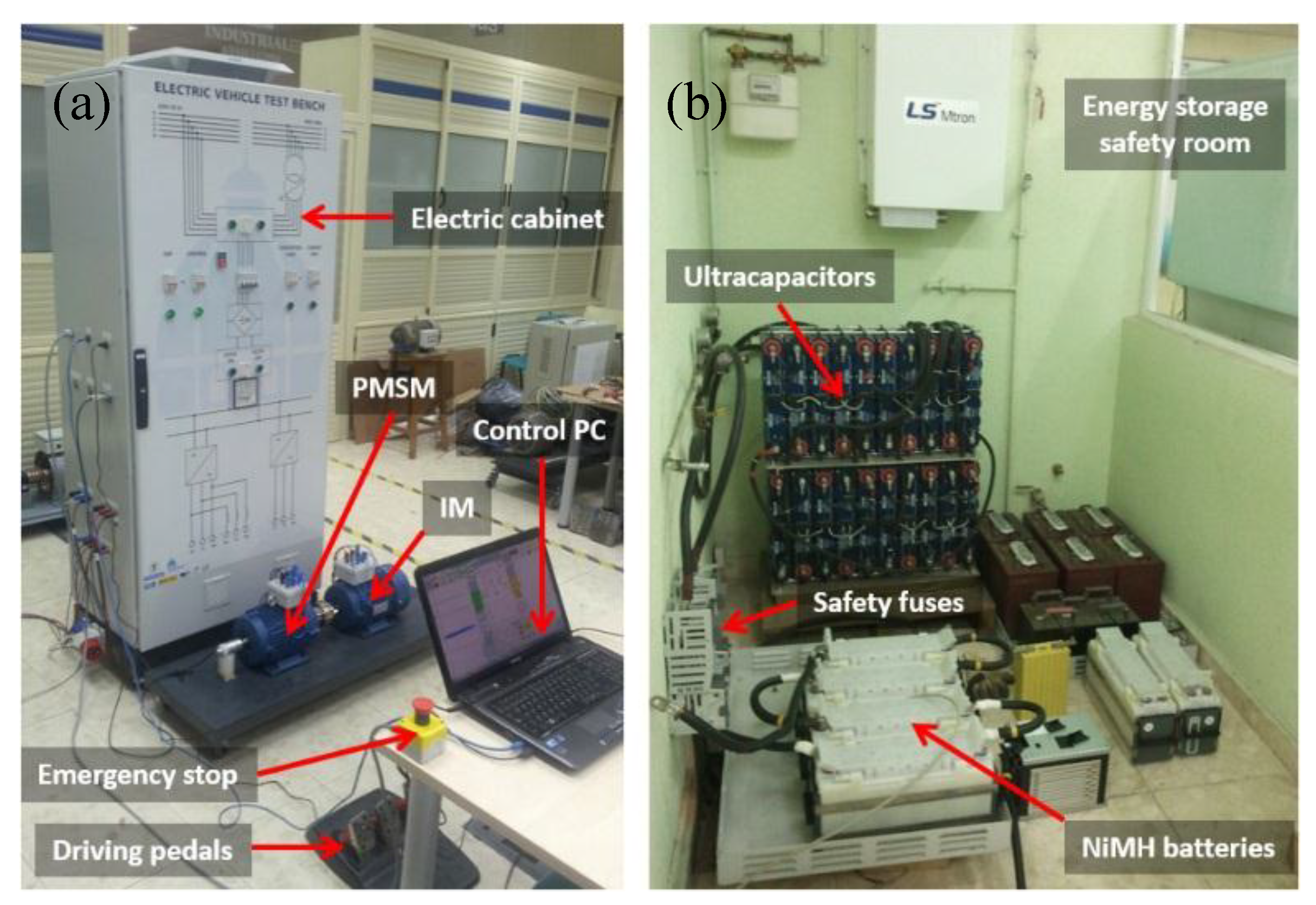Figure 8 shows a picture of the test bench, driving pedals included.

Figure 8. Laboratory test bench: (a) Electric cabinet containing three power electronic converters, bench with a PMSM (traction machine) and a IM (emulator machine), and driving pedals; (b) safety room for batteries and ultracapacitors.

Figure 8. Laboratory test bench: (a) Electric cabinet containing three power electronic converters, bench with a PMSM (traction machine) and a IM (emulator machine), and driving pedals; (b) safety room for batteries and ultracapacitors.

Three power electronic converters are needed in the test bench because of the inclusion of the vehicle emulator, which consists of the IM driven by a second inverter. Both inverters feed from the same DC link, so that power is recirculated when any of the machines is in generator mode, minimizing energy consumption from the batteries. Table 1 contains some rated values for the main devices comprising the test bench.

Table 1. Teaching Laboratory Platform: Nominal Values.

Traction machine		Load machine (emulator)
Type	Interior PMSM	Type	Squirrel cage IM
Power	3.3 kW	Power	2.2 kW
Speed	1500 rpm	Speed	1420 rpm
Pole pairs	2	Pole pairs	2
Voltage	400 VRMS	Voltage	400 VRMS
Stator current	4.84 ARMS	Stator current	4.84 ARMS
Inertia	0.0068 kg·m2	Inertia	0.0075 kg·m2
Power converters		Batteries
Type	IGBT module	Type	NiMH c
DC voltage	380 VDC a	Voltage (total)	120 V (10 × 12)
Current	60 ARMS	Capacity @C/3	100 Ah
Switch. freq.	20 kHz (max)
Emulated EV		Aerodynamics and rolling
Type	Fictitious car	Air density ρ	1.2 kg/m3
Total mass M	1200 kg	AF	1.89 m2
Max speed b	51.3 km/h	CD	0.37
ERR	0.25 m	µroll,0	0.0135
iGEAR	17.544	µroll,S	0.0055
µGEAR	95%

^a Both motors are operated with reduced voltage. Maximum speed under these circumstances (380 V_DC, no flux weakening) is 1000 rpm; ^b @1000 rpm, according to previous note; ^c For safety reasons, lithium batteries are replaced by NiMH batteries in the laboratory test bench.

Table 1. Teaching Laboratory Platform: Nominal Values.

Traction machine		Load machine (emulator)
Type	Interior PMSM	Type	Squirrel cage IM
Power	3.3 kW	Power	2.2 kW
Speed	1500 rpm	Speed	1420 rpm
Pole pairs	2	Pole pairs	2
Voltage	400 VRMS	Voltage	400 VRMS
Stator current	4.84 ARMS	Stator current	4.84 ARMS
Inertia	0.0068 kg·m2	Inertia	0.0075 kg·m2
Power converters		Batteries
Type	IGBT module	Type	NiMH c
DC voltage	380 VDC a	Voltage (total)	120 V (10 × 12)
Current	60 ARMS	Capacity @C/3	100 Ah
Switch. freq.	20 kHz (max)
Emulated EV		Aerodynamics and rolling
Type	Fictitious car	Air density ρ	1.2 kg/m3
Total mass M	1200 kg	AF	1.89 m2
Max speed b	51.3 km/h	CD	0.37
ERR	0.25 m	µroll,0	0.0135
iGEAR	17.544	µroll,S	0.0055
µGEAR	95%

^a Both motors are operated with reduced voltage. Maximum speed under these circumstances (380 V_DC, no flux weakening) is 1000 rpm; ^b @1000 rpm, according to previous note; ^c For safety reasons, lithium batteries are replaced by NiMH batteries in the laboratory test bench.

Similarly to the PMSM inverter, the modulation strategy for the IM inverter is also a conventional hysteresis-band current control with single fixed band. The control scheme has two levels as well. The lower level, the inverter controller, is responsible for the modulation technique. The upper level is the torque controller, which determines a current reference [I_sd*, I_sq*] in dq coordinates (rotor magnetizing current reference frame for the IM [20]) by means of the following expressions:

$$\begin{gathered} {{\text{I}}_{\text{sd}}}^{\text{*}}=\text{constant} \\ {{\text{I}}_{\text{sq}}}^{\text{*}}=\frac{{\text{T}}_{\text{load}}+{\text{T}}_{\text{inertia}}}{{\text{K}}_{\text{T}}} \end{gathered}$$

(16)

where T_load (Nm) is given by Equation (14) and K_T [Nm/A] is the torque constant of the IM (supposing linearity; i.e., torque is directly proportional to q-axis current for a given d-axis current). Magnetizing current I_sd^* is set to its rated value, so the torque provided by the IM is controlled by means of I_sq exclusively. T_inertia (Nm) is a fictitious torque that emulates the inertia of the vehicle, as expressed in:

$${\mathrm{J}}_{\text{emu}}={\mathrm{J}}_{\text{vehicle}}-{\mathrm{J}}_{\text{mot}}$$

(17)

$${\text{T}}_{\text{inertia}}={\mathrm{J}}_{\text{emu}}\times \frac{{\text{d}\mathrm{\omega }}_{\text{mec}}}{\text{dt}}$$

(18)

where J_emu is the part of the inertia to be emulated, J_vehicle is the total inertia of the vehicle (as seen by the traction machine) and J_mot is the actual inertia of the test bench (PMSM rotor + IM rotor + shaft).

5.2. Teaching Methodology and Case Study

In order to familiarize the students with the platform, a complete user guide for the system operation is provided to them in advance. This guide contains the description and technical characteristics of all the system components, so that they become familiar with the test bench even before going to the laboratory. Once in the practical session, and always under supervision, the students are asked to perform the following tasks:

(1)

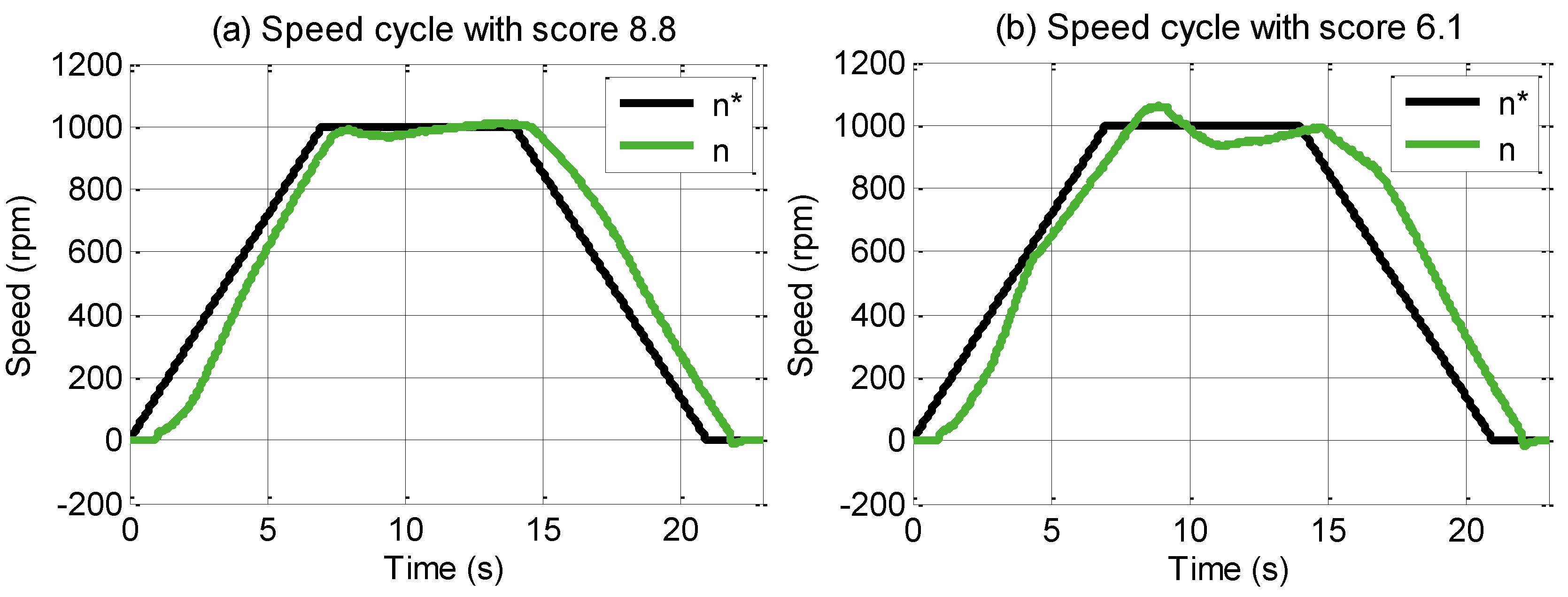
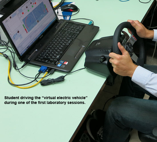
First, the students take turns to drive the “virtual electric vehicle”. They must follow a certain urban driving cycle by controlling the drive speed via the accelerator and brake pedals. This urban cycle lasts for one minute and consists in a few accelerations and brakings. In order to increase motivation, each student is given a score that values their performance as drivers once the driving cycle is finished (see example in Figure 9).

Figure 9. First exercise: 60-s driving cycle with pedals (only the first 23 s are shown). (a) Good driver (score: 8.8/10); (b) Not so good a driver (score: 6.1/10).

Figure 9. First exercise: 60-s driving cycle with pedals (only the first 23 s are shown). (a) Good driver (score: 8.8/10); (b) Not so good a driver (score: 6.1/10).

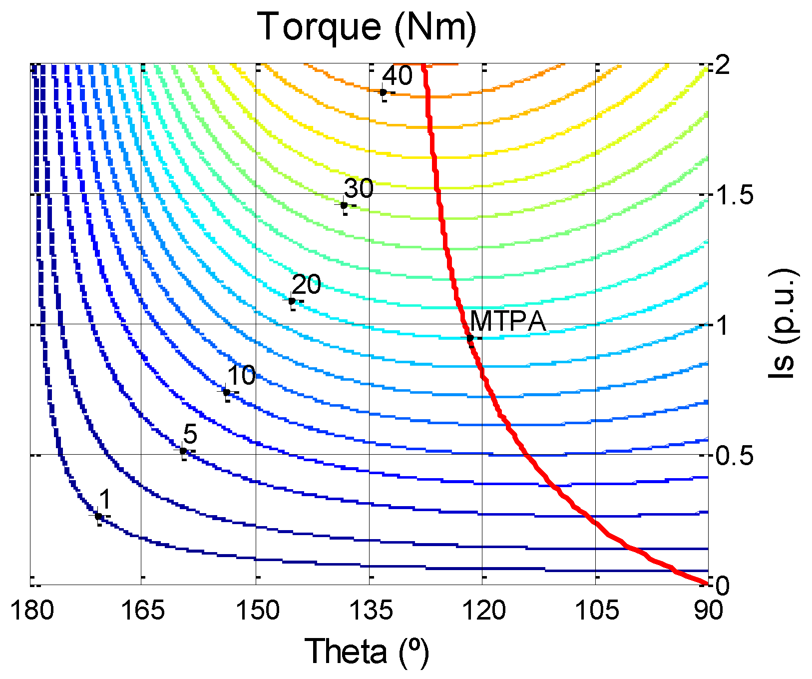
The exact cycle that each student must follow is chosen randomly from four pre-defined cycles, thus preventing them from memorizing the cycle. Each student drives the cycle two times: the first one with the MTPA trajectory disabled (I_d* = 0) and the second one with the MTPA enabled (I_d* < 0). This way, they can feel the difference between the two control strategies, as the second one is livelier (i.e., the pedals need to be pressed more intensely in the first driving cycle). Besides, since the students already modified the simulation to include the MTPA trajectory, this serves as an example of how the simulation model may be used to develop new control strategies, which is precisely what they will do in the last exercise described later in this section.

The PC controlling the test bench has two monitors. The first one displays all the information needed by the driver (e.g., speed reference and actual speed, pedals statuses and score), while the second one shows electrical magnitudes of interest (e.g., phase currents and dq currents of both machines, motor torque and emulator torque). While one of the students is driving, the rest can watch the evolution of these electrical magnitudes in the second screen and become familiar with the system operation.

(2)

Next, each team implements their chosen control improvement in the test bench assisted by the teacher. Since the control hardware is based on a dSPACE development board (MicroAutoBox II) [32], almost no extra programming needs to be done to implement what the students already developed in Simulink^®. The control interface, programmed in dSPACE ControlDesk^® Next Generation, is also highly reusable, further shortening the implementation time.

(3)

Finally, each team drives the urban cycle of the first exercise again, but with the control modifications implemented in the previous point. Before driving, each team explains to the rest what they have done and what improvement they expect to achieve. This way, all the students learn from what each team has done, regardless of their success.

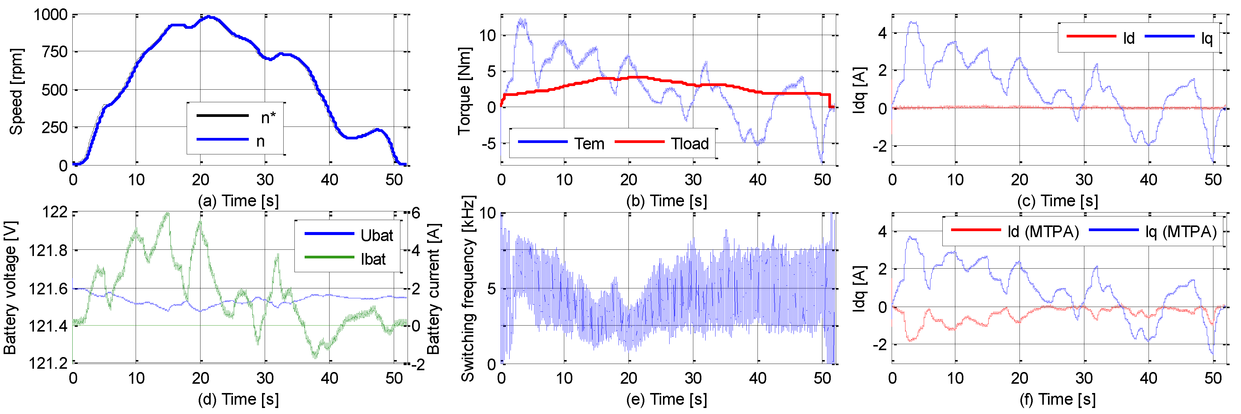
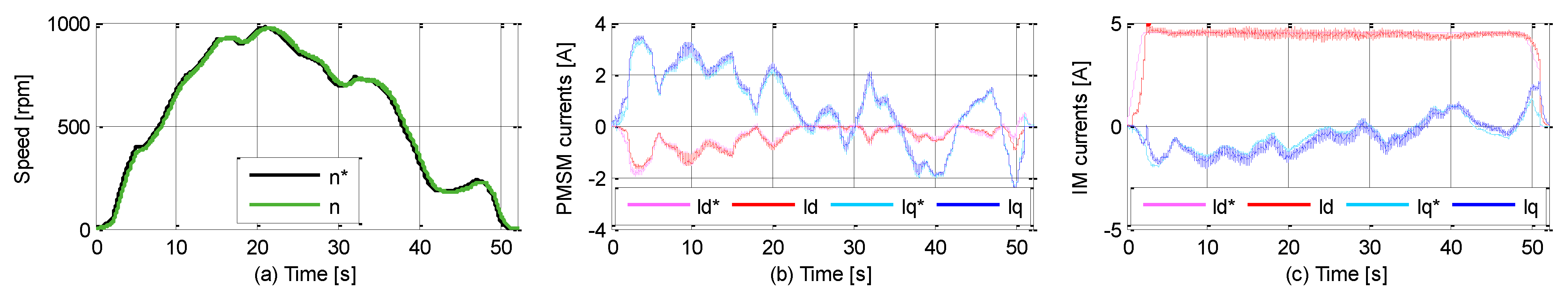
As an example of the platform capabilities, a case study is presented next. Figure 10 shows laboratory results for the same vehicle and urban cycle that were implemented in the simulation presented in previous section (Figure 7). Speed Figure 10a and PMSM currents Figure 10b are very close to those obtained in the simulation. IM currents, responsible for generating the load torque, are also depicted in Figure 10c.

Figure 10. ARTEMIS driving cycle laboratory test (only the first 52 s are shown). (a) Mechanical speed; (b) PMSM dq currents; (c) IM dq currents.

Figure 10. ARTEMIS driving cycle laboratory test (only the first 52 s are shown). (a) Mechanical speed; (b) PMSM dq currents; (c) IM dq currents.

6. Teaching Results

6.1. Course Assessment

The proposed learning project have been applied to the EVs course (which is assessed annually) during the last three years. The number of students was always very low, from 8 to 12. This was done on purpose to better follow the course development and the students’ progression during the first years after the implementation of the proposed activity. Overall, the teaching platform may be considered successful, given that both the teachers and the students think that they have a better understanding of an EV powertrain and its control since this educational project was included within the EVs course.

However, over these three years, some difficulties of practical nature have been observed. First, the course cannot support a large number of students, given that it is very time-consuming for the teachers, who need to dedicate a few hours to supervise each team of students. Secondly, the students find it very difficult to think of possible control improvements beyond those suggested by the teachers, despite what they had studied in more elementary courses. A lack of previous formation justifies this in the case of mechanical engineering students. Thirdly, the number of hours the students need to dedicate is higher than originally expected. This is because the level of understanding needed to improve the control strategy is higher than the level of understanding needed just to analyze a certain control strategy.

6.2. Students’ Feedback

Students were asked to provide informal feedback at the conclusion of the practical class. Their answers indicated that the activity was interesting, very powerful from the learning point of view but probably too time-consuming. The most common issue reported by the students is the high workload.

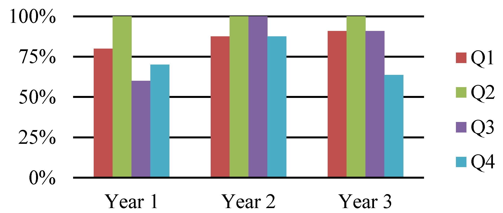
Besides, the students were asked to answer an anonymous questionnaire (yes/no answer) with four simple questions:

(Q1)

Did this course help you understand electric traction drives and their control?

(Q2)

Do you think that you have learned more after the inclusion of this practical session (when compared to a conventional course)?

(Q3)

Are you satisfied with the simulation platform?

(Q4)

Are you satisfied with the laboratory platform?

Note that Q2 asks the students to compare their current experience (the proposed activity) with an experience they have not had (such as the previous version of the course). Unfortunately, there is not enough data regarding the previous version of the course to assess how the proposed activity improves the students’ experience by comparing both feedbacks, so Q2 is used instead.

Results for this questionnaire are shown in Figure 11. The students’ response to the first two questions is clearly positive, a minority of them preferring more conventional practical sessions.

Figure 11. Student survey results.

Figure 11. Student survey results.

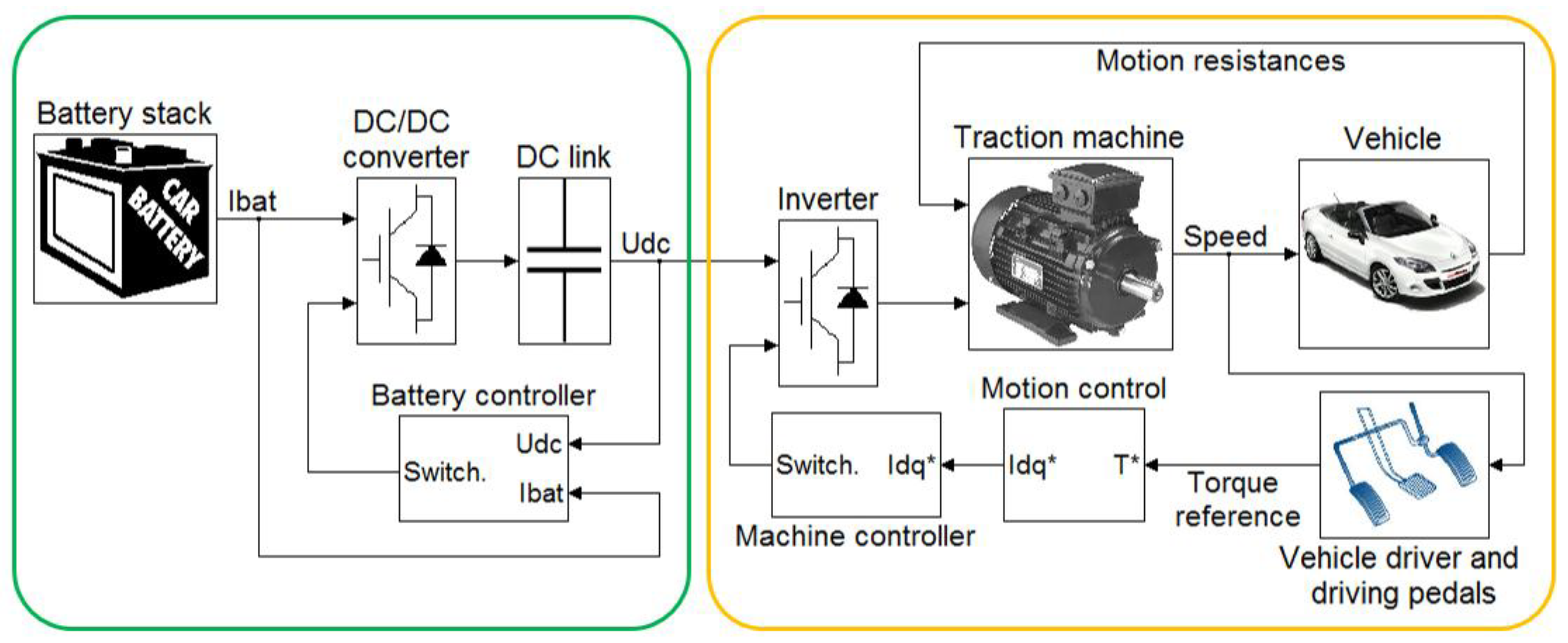
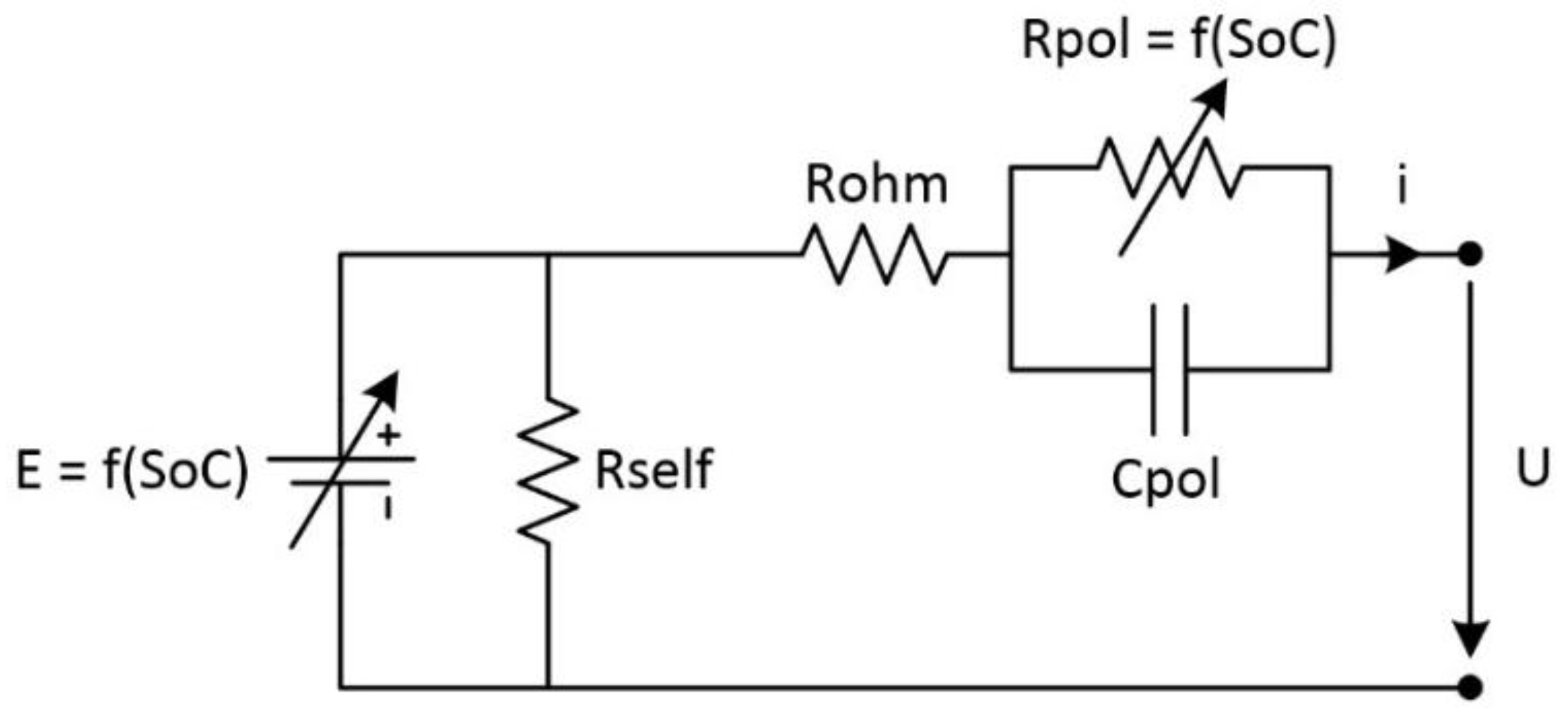
Regarding Q3, many students complained the first year about the time required for the simulation model to run (up to 30 min in an average computer, which was too much for the students to test as many control strategies as possible). The model was improved in this sense after the first year, thanks to the elimination of the energy storage part of the model (see Figure 2), thus halving the time needed to simulate and improving the students’ feedback in years 2 and 3.

Another flaw pointed out by the students is the number of laboratory platforms available (just one), which is the reason why Q4 gets the worse feedback overall, especially when the number of students is large. Some of them suggested that at least a second platform would be needed in order to optimize the time spent in the laboratory. While this is true, replicating the original platform is costly and may require the attendance of a second teacher to the laboratory sessions.

7. Conclusions

A two-level (simulation + laboratory) educational platform has been developed in order to improve the learning process on electrical traction drives and their control. The teaching methodology focus on the students’ interaction with the platform, both the simulation model and the laboratory test bench. This educational tool is intended to complement theoretical lessons.

In the simulation stage, the students develop their own control strategies/switching techniques. The most promising results are later implemented in the test bench during the laboratory stage. The students have the chance of comparing these control strategies not only by testing them, but also by driving a virtual EV by means of an accelerator and a braking pedal. This methodology has been tested in a Master’s course during three years. Both teachers and students feel that this platform improves the students’ understanding in electrical traction drives and their control. Its main drawback is the limitation in the number of students per class.

References

- Heffernan, B.; Duke, R.; Zhang, R.; Gaynor, P.; Cusdin, M. A go-cart as an electric vehicle for undergraduate teaching and assessment. In Proceedings of the 20th Australasian Universities Power Engineering Conference (AUPEC 2010), Christchurch, New Zealand, 5–8 December 2010; IEEE: New York, NY, USA, 2010. [Google Scholar]
- Reddy, G.N. An EV-simulator for electric vehicle education. In Proceedings of the International Conference on Engineering Education (ICEED 2009), Kuala Lumpur, Malaysia, 7–8 December 2009; IEEE: New York, NY, USA, 2009. [Google Scholar]
- Prasanth, V.; Bauer, P.; Ildikó, P. Drivetrain of electric car: Development of virtual lab for E-learning. In Proceedings of the IEEE International Workshop on Advanced Motion Control, Sarajevo, Bosnia and Herzegovina, Yugoslavia, 25–27 March 2012; IEEE: New York, NY, USA, 2012. [Google Scholar]
- Schafer, U. Electric vehicles—Educational aspects. In Proceedings of the XXth International Conference on Electrical Machines (ICEM 2012), Marseille, France, 2–5 September 2012; IEEE: New York, NY, USA, 2012. [Google Scholar]
- Kumar, A.; Fernando, S.; Panicker, R.C. Project-based learning in embedded systems education using an FPGA platform. IEEE Trans. Educ. 2013, 56, 407–415. [Google Scholar] [CrossRef]
- Ferrater-Simon, C.; Molas-Balada, L.; Gomis-Bellmunt, O.; Lorenzo-Martinez, N.; Bayo-Puxan, O.; Villafafila-Robles, R. A remote laboratory platform for electrical drive control using programmable logic controllers. IEEE Trans. Educ. 2009, 52, 425–435. [Google Scholar] [CrossRef]
- Oriti, G.; Julian, A.L.; Zulaic, D. Doubly fed induction machine drive hardware laboratory for distance learning education. IEEE Trans. Power Electron. 2014, 29, 440–448. [Google Scholar] [CrossRef]
- Arribas, J.R.; Veganzones, C.; Blazquez, F.; Platero, C.A.; Ramirez, D.; Martinez, S.; Sanchez, J.A.; Herrero Martinez, N. Computer-based simulation and scaled laboratory bench system for the teaching and training of engineers on the control of doubly fed induction wind generators. IEEE Trans. Power Syst. 2011, 26, 1534–1543. [Google Scholar] [CrossRef]
- Bouscayrol, A.; Guillaud, X.; Delarue, P.; Lemaire-Semail, B. Energetic macroscopic representation and inversion-based control illustrated on a wind energy conversion systems using hardware-in-the-loop simulation. IEEE Trans. Ind. Electron. 2009, 56, 4826–4835. [Google Scholar] [CrossRef]
- He, H.-W.; Xiong, R.; Chang, Y.-H. Dynamic modeling and simulation on a hybrid power system for electric vehicle applications. Energies 2010, 3, 1821–1830. [Google Scholar] [CrossRef]
- Chan, C.C.; Bouscayrol, A.; Chen, K. Electric, hybrid, and fuel-cell vehicles: Architectures and modeling. IEEE Trans. Vehicular Technol. 2010, 59, 589–598. [Google Scholar] [CrossRef]
- Mohan, G.; Assadian, F.; Longo, S. An optimization framework for comparative analysis of multiple vehicle powertrains. Energies 2013, 6, 5507–5537. [Google Scholar] [CrossRef] [Green Version]
- MathWorks, MatLab R2014a Documentation Center. Available online: http://www.mathworks.com/help/physmod/sps/index.html (accessed on 31 October 2014).
- Tremblay, O.; Dessaint, L.-A. Experimental validation of a battery dynamic model for EV applications. World Electr. Veh. J. 2009, 3, 1–10. [Google Scholar]
- Chen, M.; Rincón-Mora, G.A. Accurate electrical battery model capable of predicting runtime and I-V performance. IEEE Trans. Energy Convers. 2006, 21, 504–511. [Google Scholar] [CrossRef]
- Semikron, SEMIX71GD12E4s IGBT Modules. Available online: http://www.semikron.com/products/product-classes/igbt-modules/detail/semix71gd12e4s-27890190.html (accessed on 2 January 2015).
- Mohan, N.; Undeland, T.; Robbins, W. Power Electronics: Converters, Applications, and Design, 3rd ed.; Wiley John & Sons, Inc.: Hoboken, NJ, USA, 2003. [Google Scholar]
- Zhang, S.; Yu, X. A unified analytical modeling of the interleaved pulse width modulation (PWM) DC-DC converter and its applications. IEEE Trans. Power Electron. 2013, 28, 5147–5158. [Google Scholar] [CrossRef]
- Kazmierkowski, M.; Franquelo, L.; Rodriguez, J.; Perez, M.; Leon, J. High-performance motor drives. IEEE Ind. Electron. Mag. 2011, 5, 6–26. [Google Scholar] [CrossRef] [Green Version]
- Krishnan, R. Electric Motor Drives: Modeling, Analysis and Control; Prentice Hall: Upper Saddle River, NJ, USA, 2001. [Google Scholar]
- Akagi, H.; Watanabe, E.H.; Aredes, M. Instantaneous Power Theory and Applications to Power Conditioning; Wiley-IEEE Press: Hoboken, NJ, USA, 2007. [Google Scholar]
- Bianchi, N. Electrical Machine Analysis Using Finite Elements; Taylor & Francis: Abingdon, UK, 2005. [Google Scholar]
- Gallegos-Lopez, G.; Hiti, S. Optimum current control in the field-weakened region for permanent magnet AC machines. In Proceedings of the IEEE Industry Applications Conference, New Orleans, LA, USA, 23–27 September 2007; IEEE: New York, NY, USA, 2007. [Google Scholar]
- Schaltz, E. Electrical vehicle design and modeling. In Electric Vehicles—Modelling and Simulations; InTech: Rijeka, Croatia, 2011; Chapter 1; pp. 1–24. [Google Scholar]
- Ehsani, M.; Gao, Y.; Emadi, A. Modern Electric, Hybrid Electric, and Fuel Cell Vehicles: Fundamentals, Theory, and Design, 2nd ed.; CRC Press: New York, NY, USA, 2009. [Google Scholar]
- Xu, Q.; Cui, S.; Song, L.; Zhang, Q. Research on the power management strategy of hybrid electric vehicles based on electric variable transmissions. Energies 2014, 7, 934–960. [Google Scholar] [CrossRef]
- Batchelor, G.K. An Introduction to Fluid Dynamics; Cambridge University Press: Cambridge, UK, 2000. [Google Scholar]
- Pacejka, H.B. Tyre and Vehicle Dynamics; Butterworth-Heinemann: Oxford, UK, 2006. [Google Scholar]
- Arango, E.; Ramos-Paja, C.A.; Calvente, J.; Giral, R.; Serna, S. Asymmetrical interleaved DC/DC switching converters for photovoltaic and fuel cell applications—Part 1: Circuit generation, analysis and design. Energies 2012, 5, 4590–4623. [Google Scholar] [CrossRef]
- Rahman, K.; Khan, M.; Choundhury, M.; Rahman, M. Variable-band hysteresis current controllers for PWM voltage-source inverters. IEEE Trans. Power Electron. 1997, 12, 964–970. [Google Scholar] [CrossRef]
- André, M. The ARTEMIS European driving cycles for measuring car pollutant emissions. Sci. Total Environ. 2004, 334–335, 73–84. [Google Scholar] [CrossRef] [PubMed]
- dSPACE Website. Available online: http://www.dspace.com/en/pub/home/products.cfm (accessed on 31 October 2014).
© 2015 by the authors; licensee MDPI, Basel, Switzerland. This article is an open access article distributed under the terms and conditions of the Creative Commons Attribution license (http://creativecommons.org/licenses/by/4.0/).