
Towards a Low-Cost Modelling System for Optimising the Layout of Tidal Turbine Arrays

Abstract
:1. Introduction
2. Methodology
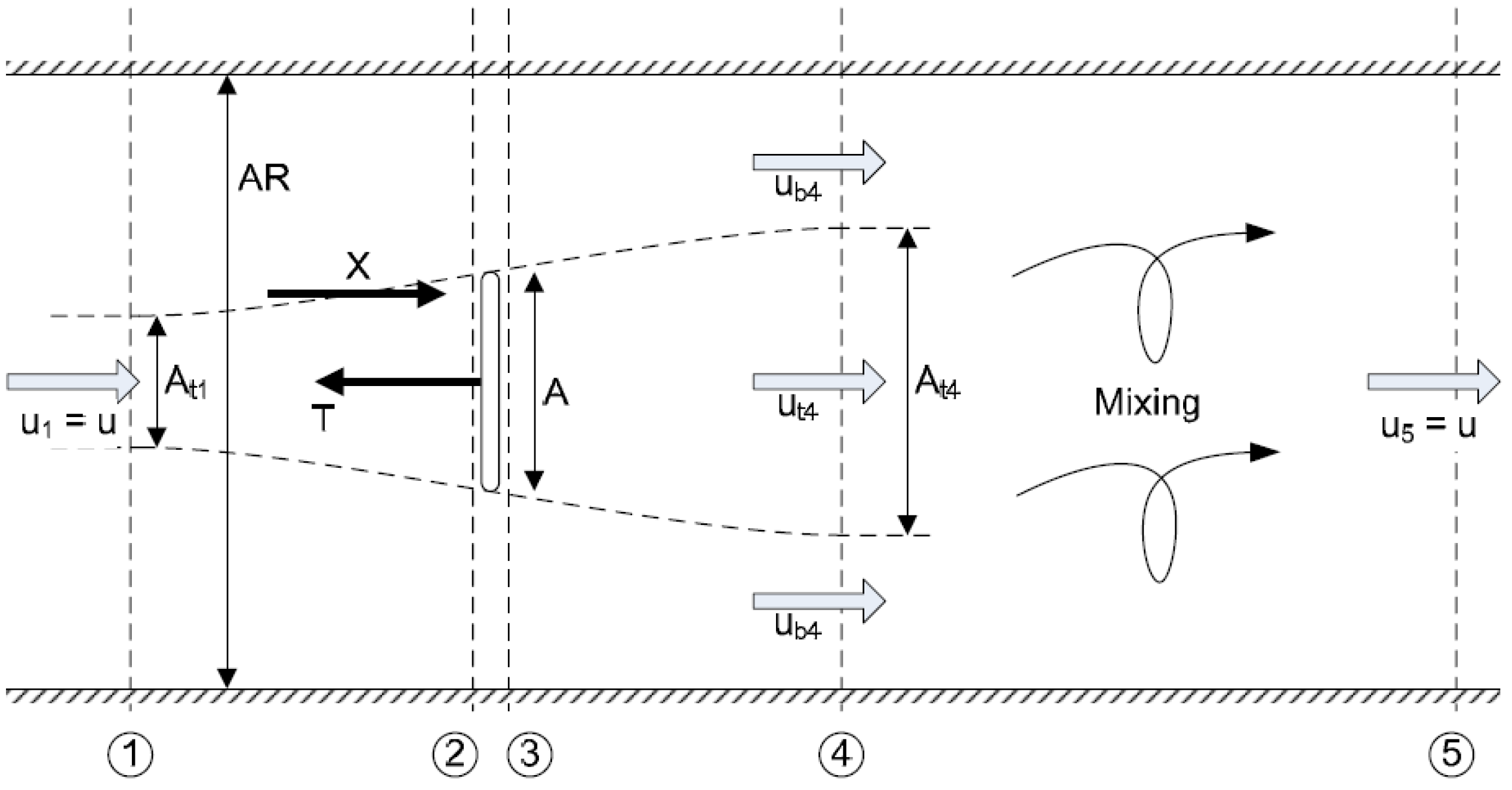
2.1. Theory

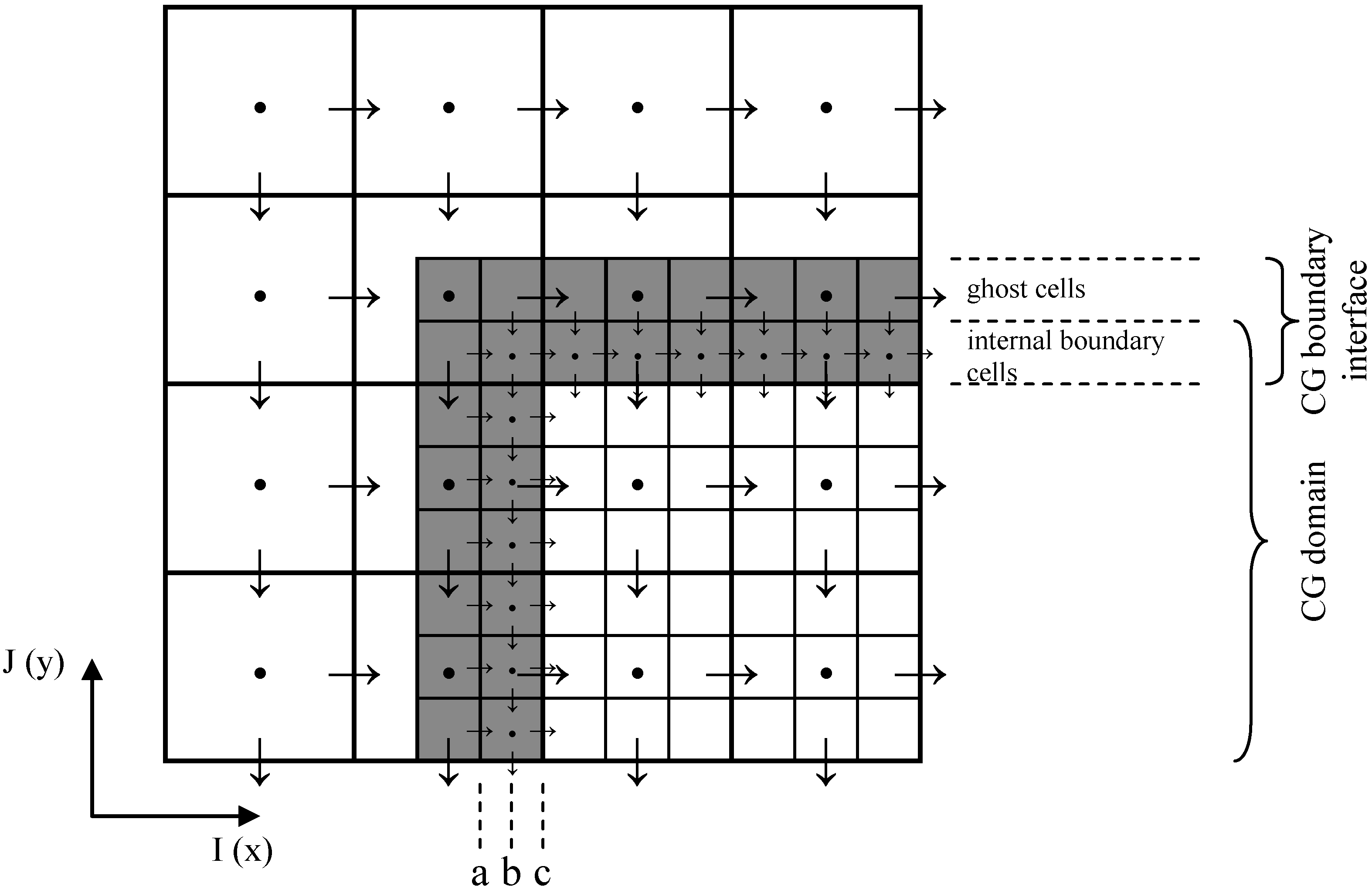
2.2. Numerical Approach to Representation of Turbines
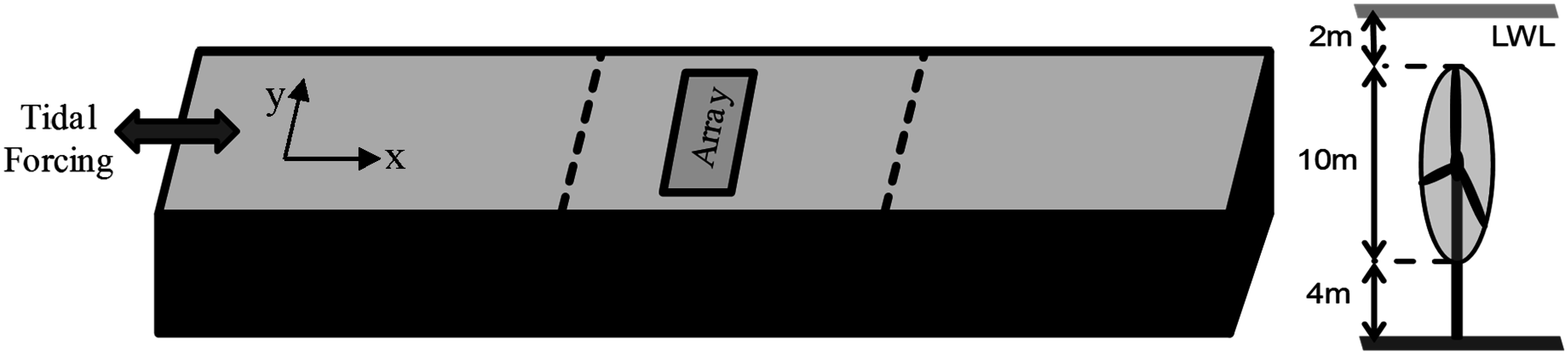
3. Numerical Simulation


| Physical Parameter | Domain | |
|---|---|---|
| Parent Grid: PG | Child Grid: CG | |
| LX | 5.0 km | 1.5 km |
| LY | 0.6 km | 0.6 km |
| Water depth | 20 m | 20 m |
| Tidal amplitude | 4 m | 4 m |
| Tidal period | 6.25 h | 6.25 h |
| Grid SPACING | 50 m | 10 m |
| Timestep | 12 s | 60 s |
| No. of grid cells | 2400 | 9000 |
| Bed roughness | 50 mm | 50 mm |
4. Numerical Simulation Results
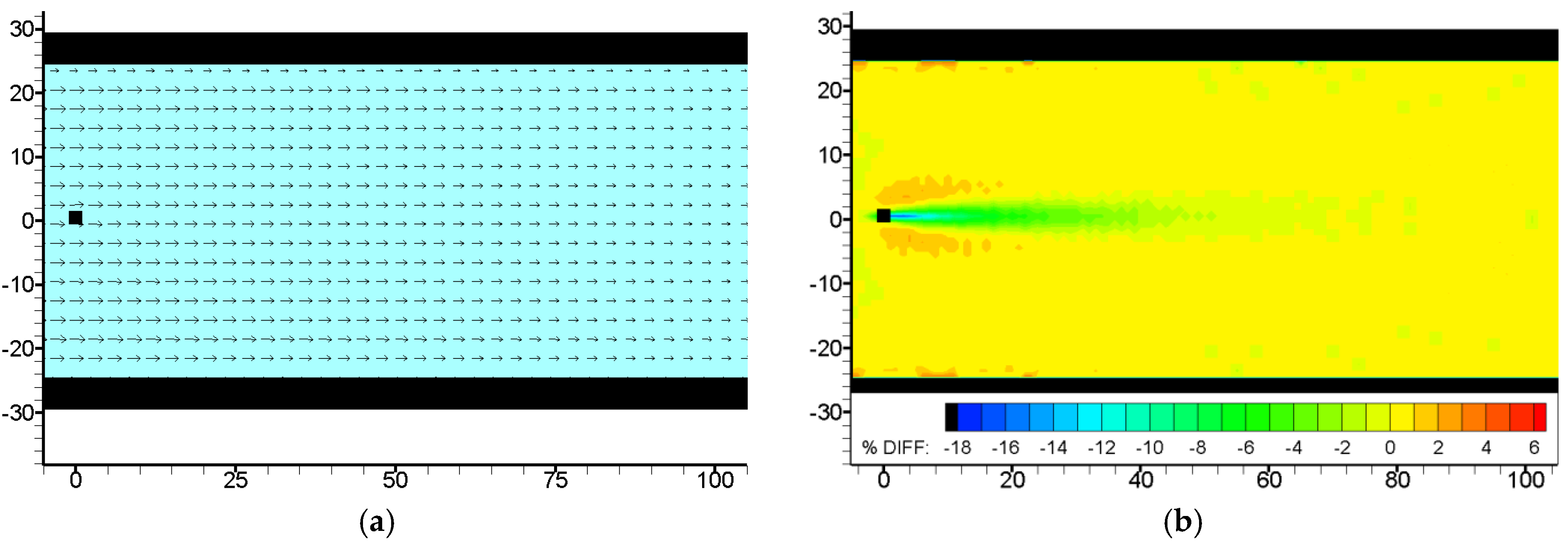
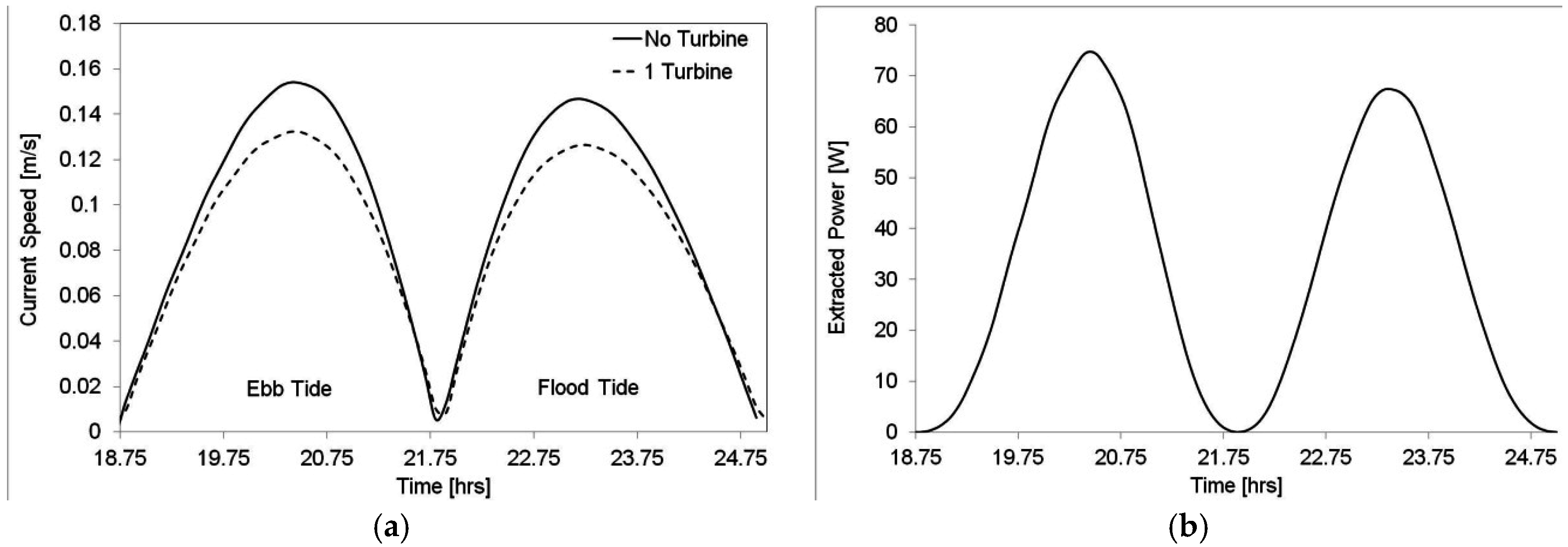
4.1. Single Turbine


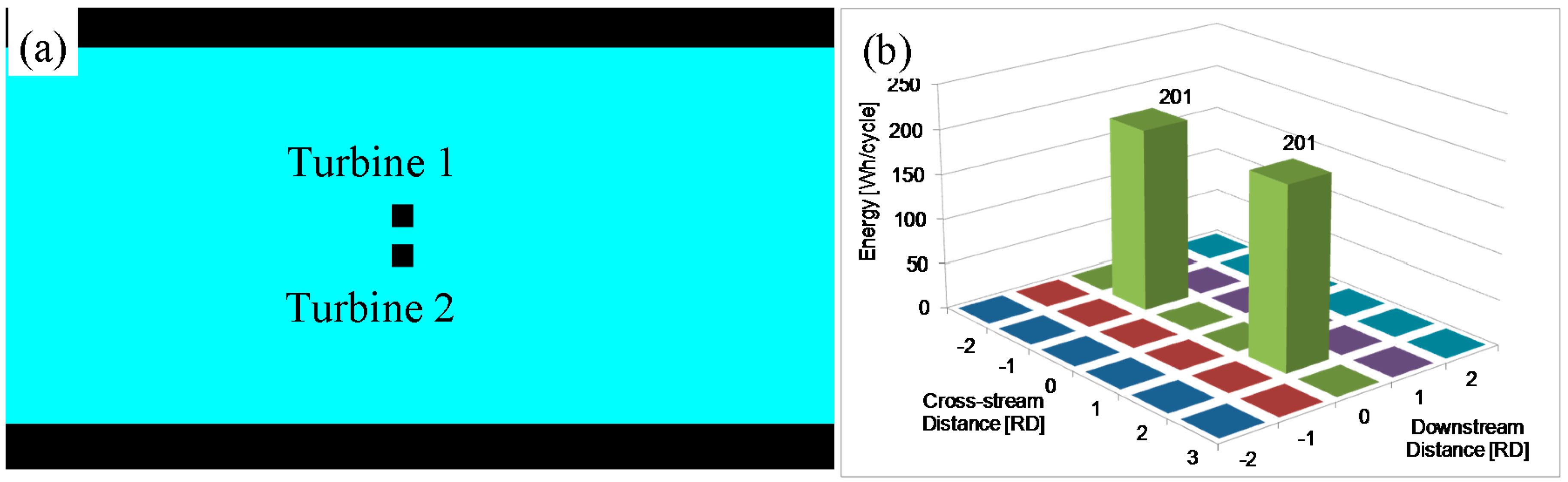
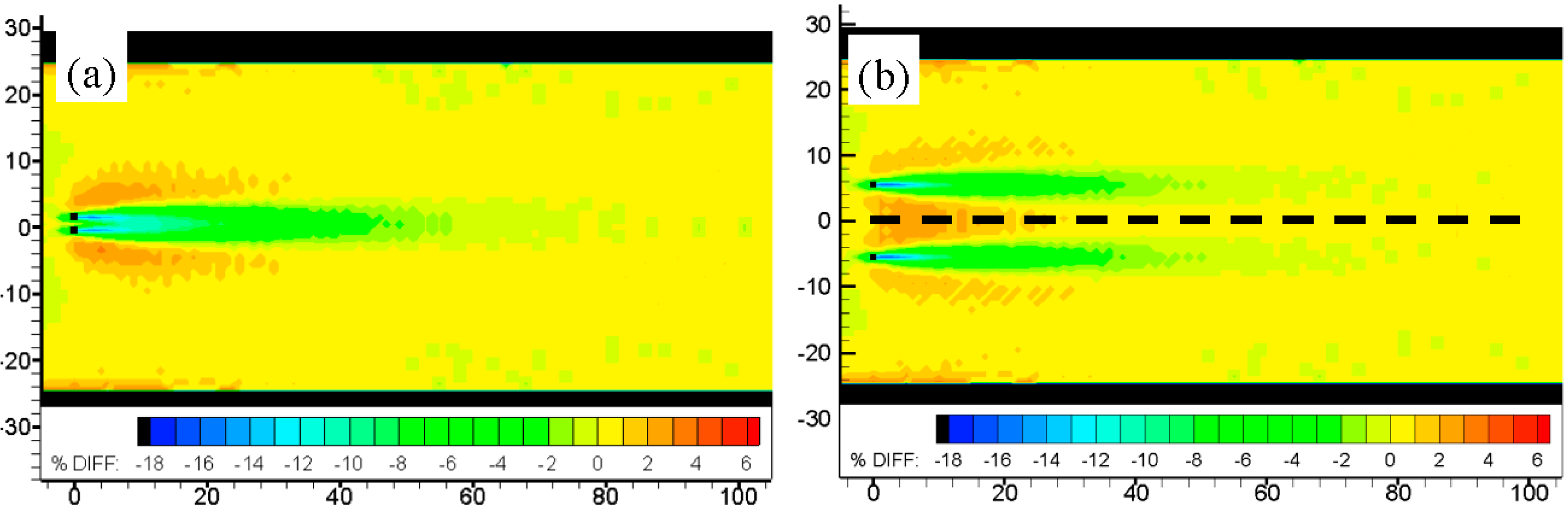
4.2. Two Turbines


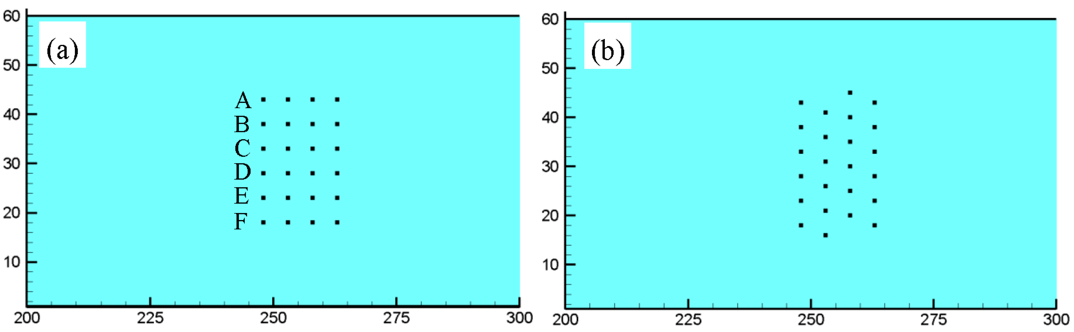
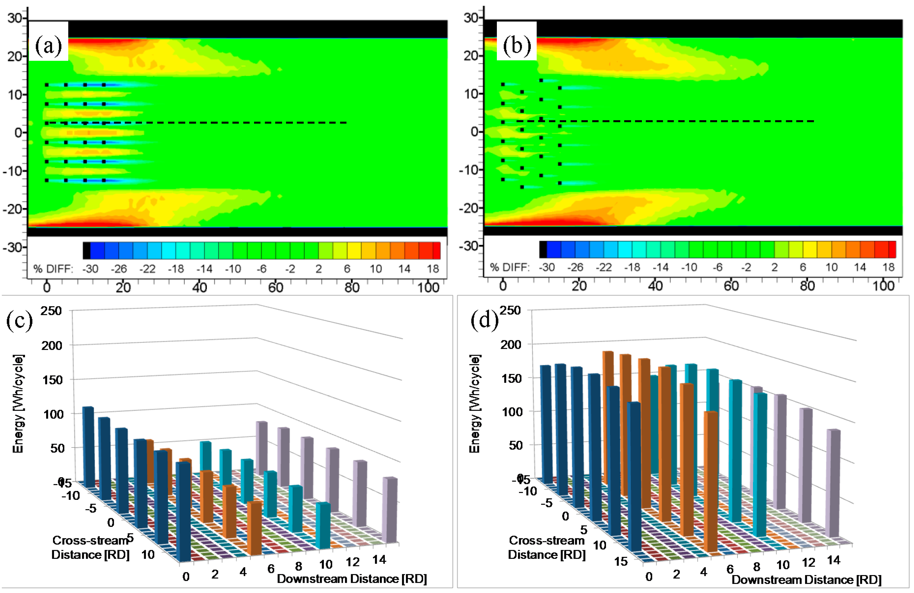
4.3. Array
- (1)
- A staggered array formation in which downstream turbines do not significantly interact with the wakes of upstream turbines thus allowing the use of a relatively small longitudinal spacing.
- (2)
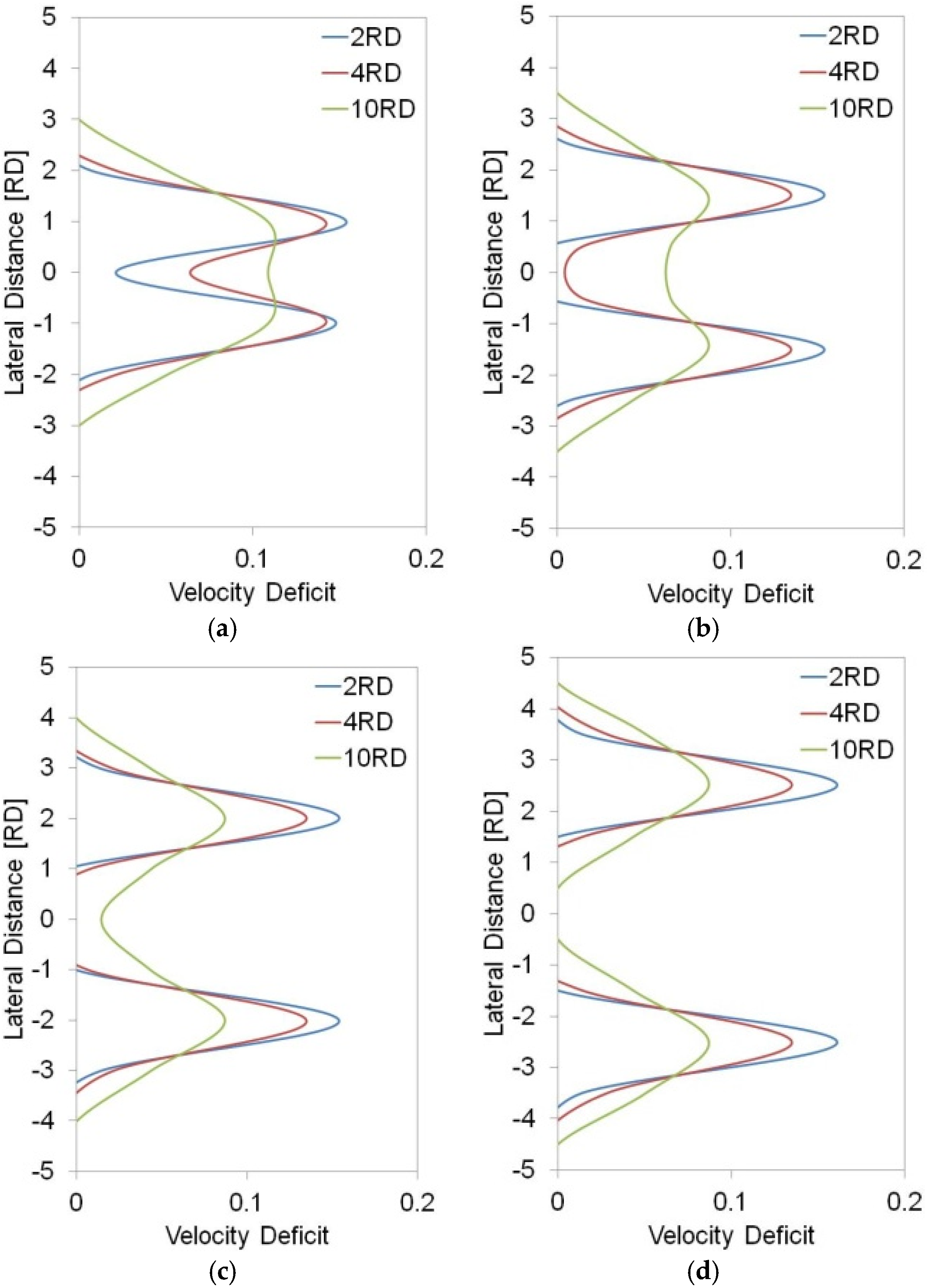
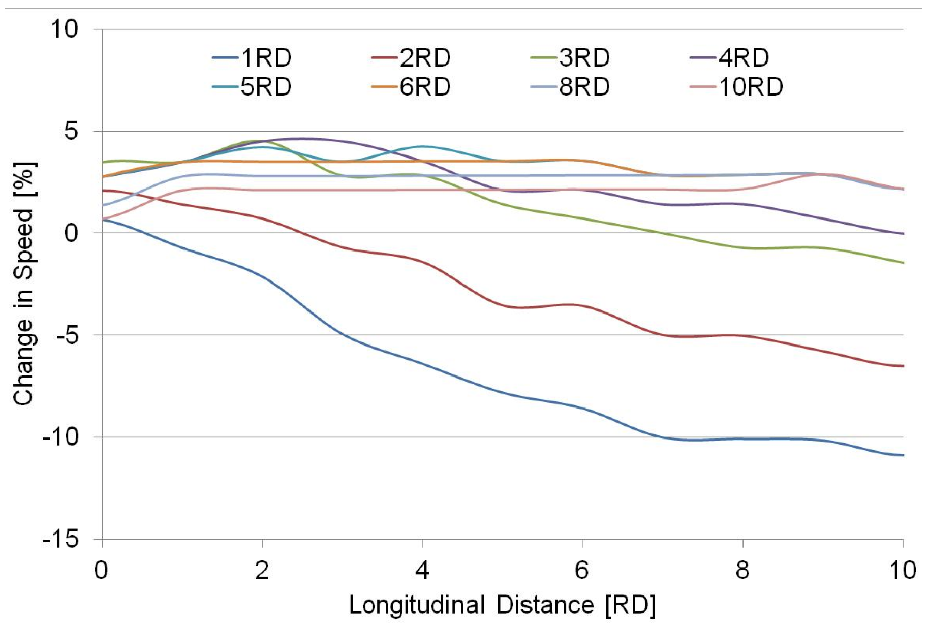
- A lateral spacing that would induce flow acceleration which downstream turbines could then intercept—the results suggested an optimal spacing of between 3 RD and 4 RD.
- (3)
- A longitudinal spacing that would place downstream turbines within the region of highest flow acceleration—the results suggested an optimal spacing of between 1 RD and 4 RD.
5. Conclusions
- Far-field models allow simulation of large multiple device arrays, and using nesting to obtain a spatial resolution equal to the simulated turbine rotor diameter allows such models to capture the wake and blockage effects of individual turbines and the resulting interactions between turbines, all of which have a significant impact on the potential energy capture of an array.
- Not-withstanding the model limitations, the modelling approach enables computation of turbine wakes of similar spatial extents and velocity deficits to those recorded in published scaled-turbine experiments. The interactions between devices computed by the model, such as wake merging and intra-turbine accelerations, also compare favourably with the same processes noted in published experimental studies.
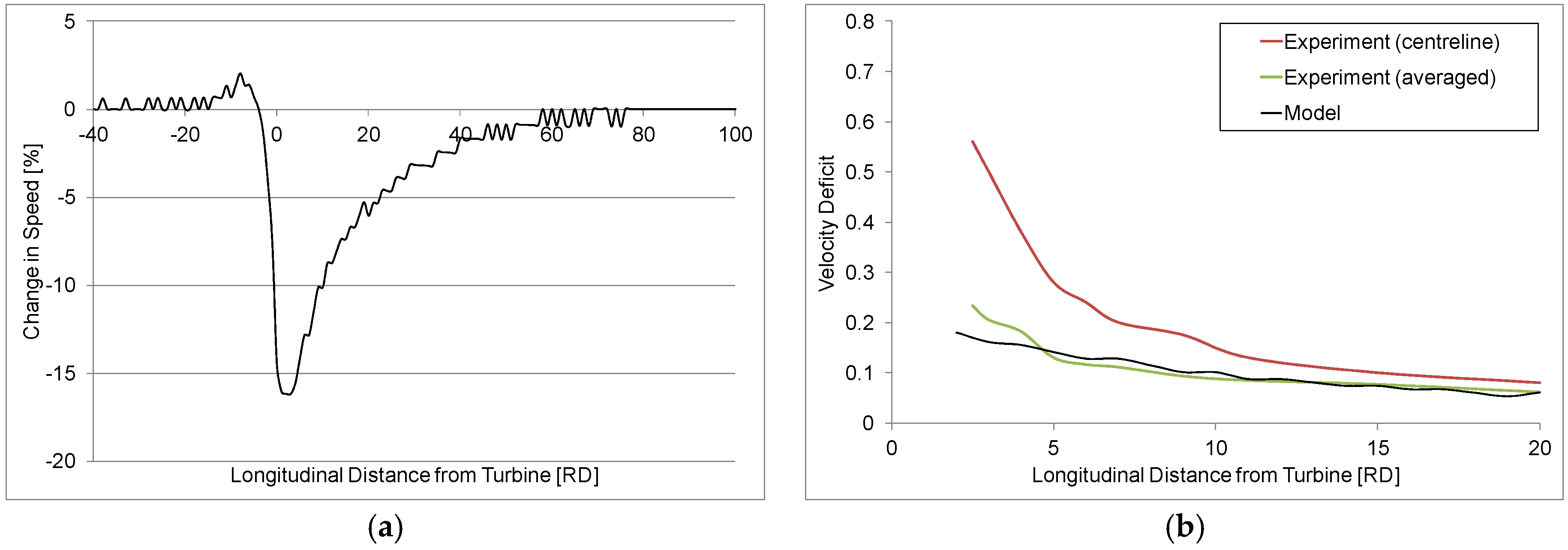
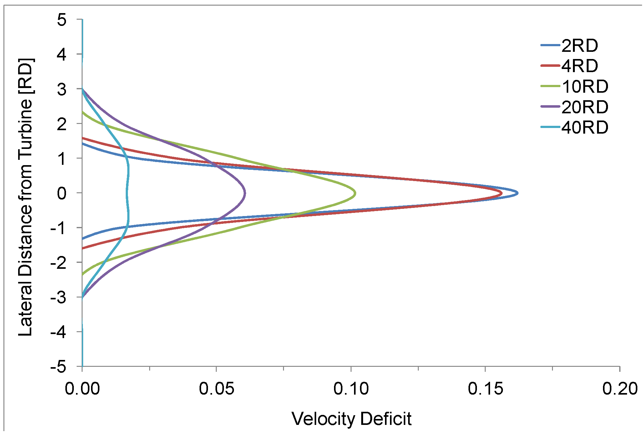
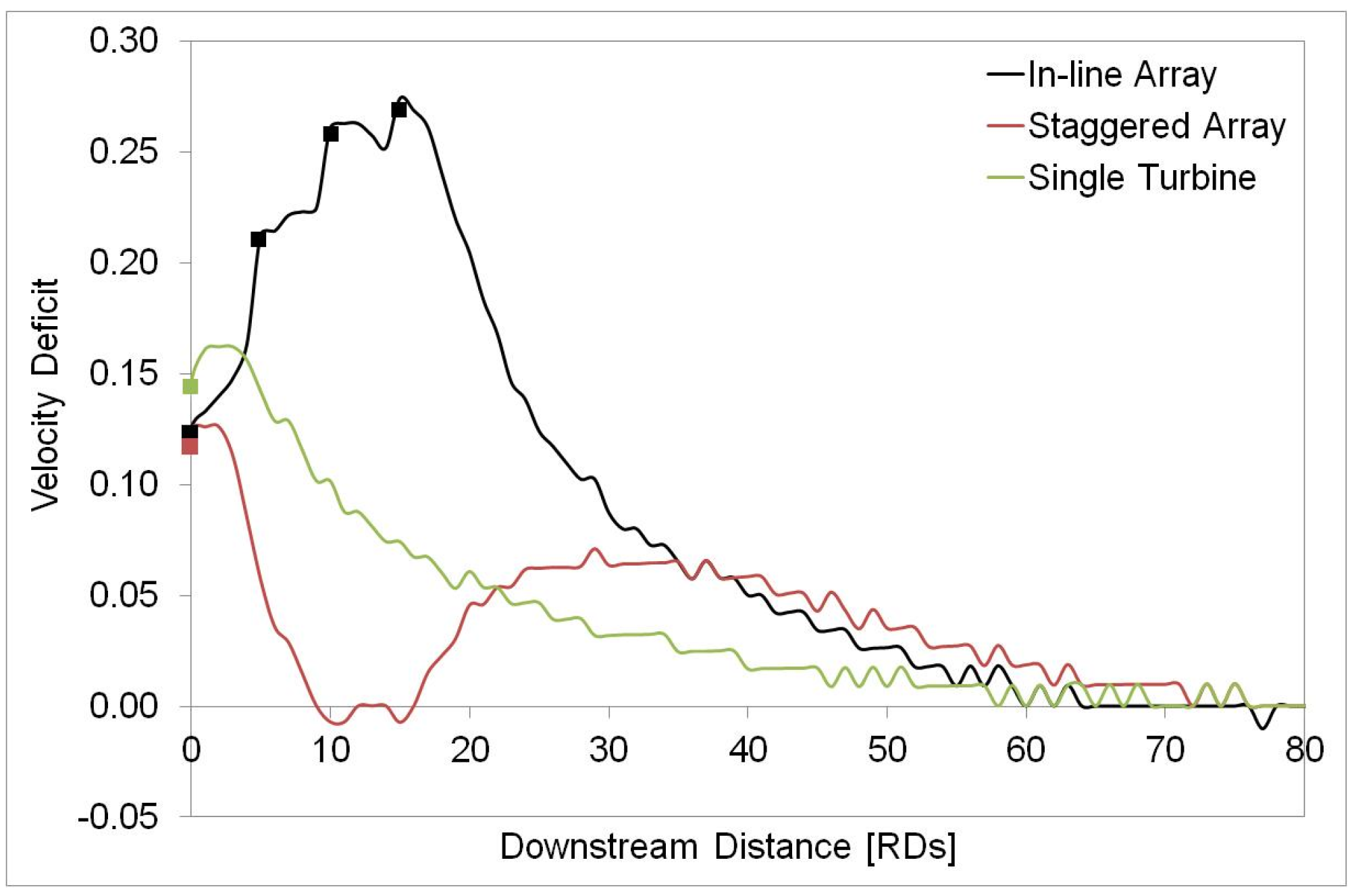
- For a single isolated turbine, deceleration of flow occurs in the turbine wake. Wake recovery, due to downstream mixing, subsequently results in the dissipation of power losses with distance downstream and a return to ambient flow conditions. Model results indicate that this occurs at a distance of approximately 70 RD; two in-line turbines placed within 70 RD of each other will therefore experience reduced power availability on either ebbing or flooding tides. Velocities were found to return to within 2% of undisturbed levels at 40 RD; this could be considered an acceptable longitudinal spacing for in-line turbines but is not practical given the limited spatial extents of high energy tidal stream sites.
- The lateral spacing between turbines can be tuned to induce flow acceleration, which can, in turn, be harnessed by appropriately placed downstream turbines. The research indicates that an optimal lateral spacing for inducing acceleration between turbines is 3 RD and 4 RD and an optimal longitudinal spacing for downstream turbines to intercept accelerated flows is 1–4 RD. The use of larger longitudinal spacings will position the downstream turbine outside of the area of peak accelerations.
- A staggered array layout is recommended, where downstream turbines are placed such that they intercept the accelerated flows induced by upstream turbines and avoid the wakes of adjacent turbines. A staggered array using 4 RD lateral and longitudinal spacings resulted in an energy yield per tidal cycle of more than twice that of a comparable in-line array.
Acknowledgments
- Marine Renewable Energy Ireland (MaREI) which is supported by Science Foundation Ireland under Grant No. 12/RC/2302.
- The MAREN2 project which is part-funded by the European Regional Development Fund (ERDF) through the Atlantic Area Transnational Programme (INTERREG IV).
- The ENERGYMARE project which is part-funded by the European Regional Development Fund (ERDF) through the Atlantic Area Transnational Programme (INTERREG IV).
Author Contributions
Conflicts of Interest
References
- Bahaj, A.S.; Molland, A.F.; Chaplin, J.R.; Batten, W.M.J. Power and thrust measurements of marine current turbines under various hydrodynamic flow conditions in a cavitation tunnel and a towing tank. Renew. Energy 2007, 32, 407–426. [Google Scholar] [CrossRef]
- Vennell, R. Tuning turbines in a tidal channel. J. Fluid Mech. 2010, 663, 253–267. [Google Scholar] [CrossRef]
- Meygen. The Meygen Project. Available online: http://www.meygen.com/ (accessed on 17 June 2013).
- Divett, T.; Vennell, R.; Stevens, C. Optimization of multiple turbine arrays in a channel with tidally reversing flow by numerical modelling with adaptive mesh. In Proceedings of the 10th European Wave and Tidal Energy Conference, Southampton, UK, 5–9 September 2011.
- Bahaj, A.S.; Myers, L.E.; Thomson, M.D.; Jorge, N. Characterising the wake of horizontal axis marine current turbines. In Proceedings of the 7th European Wave and Tidal Energy Conference, Porto, Portugal, 11–14 September 2007.
- Sun, X.; Chick, J.P.; Bryden, I.G. Laboratory-scale simulation of energy extraction from tidal currents. Renew. Energy 2008, 33, 1267–1274. [Google Scholar] [CrossRef]
- McNaughton, J.; Afgan, I.; Apsley, D.D.; Rolfo, S.; Stallard, T.; Stansby, P.K. A simple sliding-mesh interface procedure and its application to the CFD simulation of a tidal-stream turbine. Int. J. Numer. Methods Fluids 2014, 74, 250–269. [Google Scholar] [CrossRef]
- Lawson, M.; Li, Y.; Sale, D. Development and verification of a computational fluid dynamics model of a horizontal-axis tidal current turbine. In Proceedings of the 30th International Conference on Ocean, Offshore, and Arctic Engineering, Rotterdam, The Netherlands, 19–24 June 2011.
- O’Doherty, D.M.; Mason-Jones, A.; O’Doherty, T.; Byrne, C.B. Considerations of improved tidal stream turbine performance using double rows of contra-rotating blades. In Proceedings of the 8th European Wave and Tidal Energy Conference, Uppsala, Sweden, 7–10 September 2009.
- Javaherchi, T.; Stelzenmuller, N.; Seydel, J.; Aliseda, A. Experimental and Numerical Analysis of a Scale-Model Horizontal Axis Hydrokinetic Turbine. In Proceedings of the 2nd Marine Energy Technology Symposium, Seattle, WA, USA, 15–17 April 2014.
- Mozafari, J.; Teymour, T. Numerical Investigation of Marine Hydrokinetic Turbines: Methodology Development for Single Turbine and Small Array Simulation, and Application to Flume and Full-Scale Reference Models. Ph.D. Thesis, University of Washington, Seattle, WA, USA, 2014. [Google Scholar]
- Willis, M.; Masters, I.; Thomas, S.; Gallie, R.; Loman, J.; Cook, A.; Ahmadian, R.; Falconer, R.; Lin, B.; Gao, G.; et al. Tidal turbine deployment in the Bristol Channel: A case study. Proc. ICE Energy 2010, 163, 93–105. [Google Scholar] [CrossRef]
- Mozafari, A.T.J. Numerical Modeling of Tidal Turbines: Methodology Development and Potential Physical Environmental Effects. Master’s Thesis, University of Washington, Seattle, WA, USA, 2010. [Google Scholar]
- Masters, I.; Williams, A.; Nick-Croft, T.; Togneri, M.; Edmunds, M.; Zangiabadi, E.; Fairley, I.; Karunarathna, H. A Comparison of Numerical Modelling Techniques for Tidal Stream Turbine Analysis. Energies 2015, 8, 7833–7853. [Google Scholar] [CrossRef]
- Draper, S.; Houlsby, G.; Oldfield, M.; Borthwick, A. Modelling tidal energy extraction in a depth averaged coastal domain. IET Renew. Power Gener. 2010, 4, 545–554. [Google Scholar] [CrossRef]
- Ahmadian, R.; Falconer, R.A. Assessment of array shape of tidal stream turbines on hydro-environmental impacts and available power. Renew. Energy 2012, 44, 318–327. [Google Scholar] [CrossRef]
- Plew, D.R.; Stevens, C.L. Numerical modelling of the effect of turbines on currents in a tidal channel—Tory Channel, New Zealand. Renew. Energy 2013, 57, 269–282. [Google Scholar] [CrossRef]
- Vogel, C.R.; Willden, R.H.J.; Houlsby, G.T. A correction for depth—Averaged simulations of tidal turbine arrays. In Proceedings of the 10th European Wave and Tidal Energy Conference (EWTEC), Aalborg, Denmark, 2–5 September 2013.
- Funke, S.W.; Farrell, P.E.; Piggott, M.D. Tidal turbine array optimisation using the adjoint approach. Renew. Energy 2014, 63, 658–673. [Google Scholar] [CrossRef]
- Divett, T.; Vennell, R.; Stevens, C. Optimization of multiple turbine arrays in a channel with tidally reversing flow by numerical modelling with adaptive mesh. Philos. Trans. R. Soc. Lond. A Math. Phys. Eng. Sci. 2013, 371. [Google Scholar] [CrossRef] [PubMed]
- Nash, S. Development of an Efficient Dynamically Nested Model for Tidal Hydraulics and Solute Transport. Ph.D. Thesis, College of Engineering & Informatics, National University of Ireland, Galway, Ireland, 2010. [Google Scholar]
- Nash, S.; Hartnett, M. Development of a nested coastal circulation model: Boundary error reduction. Environ. Model. Softw. 2014, 53, 65–80. [Google Scholar] [CrossRef]
- Nash, S.; Hartnett, M. Nested circulation modelling of inter-tidal zones: Details of a nesting approach incorporating moving boundaries. Ocean Dyn. 2010, 60, 1479–1495. [Google Scholar] [CrossRef]
- Falconer, R.A. A mathematical model study of the flushing characteristics of a shallow tidal bay. Proc. Inst. Civil Eng. 1984, 77, 311–332. [Google Scholar] [CrossRef]
- Hartnett, M.; Nash, S.; Olbert, I. An integrated approach to trophic assessment of coastal waters incorporating measurement, modelling and water quality classification. Estuar. Coast. Shelf Sci. 2012, 112, 126–138. [Google Scholar] [CrossRef]
- Nash, S.; Hartnett, M.; Dabrowski, T. Modelling phytoplankton dynamics in a complex estuarine system. Proc. ICE Water Manag. 2010, 164, 35–54. [Google Scholar] [CrossRef]
- Nishino, T.; Willden, R.H.J. Two-scale dynamics of flow past a partial cross-stream array of tidal turbines. J. Fluid Mech. 2013, 730, 220–244. [Google Scholar] [CrossRef]
- Houlsby, G.T.; Draper, S.; Oldfield, M.L.G. Application of Linear Momentum Actuator Disc Theory to Open Channel Flow; Report No OUEL 2296/08; University of Oxford: Oxford, UK, 2008. [Google Scholar]
- Fallon, D.; Hartnett, M.; Olbert, A.; Nash, S. The effects of array configuration on the hydro-environmental impacts of tidal turbines. Renew. Energy 2014, 64, 10–25. [Google Scholar] [CrossRef]
- Sutherland, G.; Foreman, M.; Garrett, C. Tidal current energy assessment for Johnstone Strait, Vancouver Island. J. Power Energy 2007, 221, 147–157. [Google Scholar] [CrossRef]
- Karsten, R.H.; McMillan, J.M.; Lickley, M.J.; Haynes, R.D. Assessment of tidal current energy in the Minas Passage, Bay of Fundy. Proc. Inst. Mech. Part A J. Power Energy 2008, 222, 493–507. [Google Scholar] [CrossRef]
- Olbert, A.I.; Nash, S.; Ragnoli, E.; Hartnett, M. Parameterization of turbulence models using 3DVAR data. In Proceedings of the 11th International Conference on Hydroinformatics, New York, NY, USA, 17–21 August 2014.
- Mason-Jones, A.; O’Doherty, D.M.; Morris, C.E.; O’Doherty, T. Influence of a velocity profile and support structure on tidal stream turbine performance. Renew. Energy 2013, 52, 23–30. [Google Scholar] [CrossRef]
- Achenbach, E. Influence of surface roughness on the cross-flow around a circular cylinder. J. Fluid Mech. 1971, 46, 321–335. [Google Scholar] [CrossRef]
- Vennell, R. Exceeding the Betz limit with tidal turbines. Renew. Energy 2013, 55, 277–285. [Google Scholar] [CrossRef]
- Stallard, T.; Collings, R.; Feng, T.; Whelan, J. Interactions between tidal turbine wakes: Experimental study of a group of three-bladed rotors. Philos. Trans. R. Soc. Lond. A Math. Phys. Eng. Sci. 2013, 371. [Google Scholar] [CrossRef] [PubMed]
- Lewis, M.J.; Neill, S.P.; Hashemi, M.R.; Reza, M. Realistic wave conditions and their influence on quantifying the tidal stream energy resource. Appl. Energy 2014, 136, 495–508. [Google Scholar] [CrossRef]
- Myers, L.E.; Bahaj, A.S. An experimental investigation simulating flow effects in first generation marine current energy converter arrays. Renew. Energy 2012, 37, 28–36. [Google Scholar] [CrossRef]
- Blackmore, T.; Batten, W.M.J.; Bahaj, A.S. Turbulence generation and its effect in LES approximations of tidal turbines. In Proceedings of the 10th European Wave and Tidal Energy Conference, Aalborg, Denmark, 2–5 September 2013.
© 2015 by the authors; licensee MDPI, Basel, Switzerland. This article is an open access article distributed under the terms and conditions of the Creative Commons by Attribution (CC-BY) license (http://creativecommons.org/licenses/by/4.0/).
Share and Cite
Nash, S.; Olbert, A.I.; Hartnett, M. Towards a Low-Cost Modelling System for Optimising the Layout of Tidal Turbine Arrays. Energies 2015, 8, 13521-13539. https://doi.org/10.3390/en81212380
Nash S, Olbert AI, Hartnett M. Towards a Low-Cost Modelling System for Optimising the Layout of Tidal Turbine Arrays. Energies. 2015; 8(12):13521-13539. https://doi.org/10.3390/en81212380
Chicago/Turabian StyleNash, Stephen, Agnieszka I. Olbert, and Michael Hartnett. 2015. "Towards a Low-Cost Modelling System for Optimising the Layout of Tidal Turbine Arrays" Energies 8, no. 12: 13521-13539. https://doi.org/10.3390/en81212380