Article

Response Based Emergency Control System for Power System Transient Stability

State Key Laboratory of Electrical Insulation and Power Equipment, School of Electrical Engineering, Xi’an Jiaotong University, No. 28, Xianning West Road, Xi’an 710049, Shaanxi, China
*
Author to whom correspondence should be addressed.
Energies 2015, 8(12), 13508-13520; https://doi.org/10.3390/en81212381
Submission received: 8 August 2015 / Revised: 11 November 2015 / Accepted: 13 November 2015 / Published: 30 November 2015
(This article belongs to the Special Issue Electric Power Systems Research)

Abstract

:
A transient stability control system for the electric power system composed of a prediction method and a control method is proposed based on trajectory information. This system, which is independent of system parameters and models, can detect the transient stability of the electric power system quickly and provide the control law when the system is unstable. Firstly, system instability is detected by the characteristic concave or convex shape of the trajectory. Secondly, the control method is proposed based on the analysis of the slope of the state plane trajectory when the power system is unstable. Two control objectives are provided according to the methods of acquiring the far end point: one is the minimal cost to restore the system to a stable state; the other one is the minimal cost to limit the maximum swing angle. The simulation indicates that the mentioned transient stability control system is efficient.

1. Introduction

This is a follow-up paper of a series on closed loop control systems for power system transient stability. The previous work proposed a real-time approach to detect transient instability with high accuracy and wide applicability, while this paper mainly focuses on how and where to control the system after the instability is detected.
In China, transient stability control systems acquire some characteristic variables according to a large number of offline calculations and identify the stability by the combination of these characteristic variables. For unstable situations, the control quantity of different situations is obtained by repeated simulations to develop a cure table. When disturbances occur, protection devices operate on the basis of the cure table [1,2].
The samples consist of different situations, including power flow, grid topology and fault conditions making it hard to ensure an effective cure table. In order to decrease the number of samples and improve the utility of the cure table, a simulation which is helpful to detect transient instability and form control law adopts measurement results to update the online power flow with a refresh cycle of 3–5 min [3,4,5,6]. Corresponding approaches has been introduced in [5,6], including preplanned remedial action and system integrity protection schemes, software processes and hardware requirements. To speed up the simulation, the transient energy function method, the equal area criterion, topological energy function or quasi-real-time online transient analysis are employed in the time domain simulation, which can greatly improve the efficiency [7,8,9,10,11,12].
In any case these methods need repeated simulations to calculate control laws by taking into account the changes in operating conditions or parameter variations. The validity of the cure table depends on the similarity between the anticipated faults and actual faults and the accuracy of the model parameters. However, a practical operating model (especially a model of the load) or the system parameters are hard to acquire. Meanwhile, the rapid development and the operation variations lead to a large number of calculation samples.
With the development of computer science and communication technology, especially the application of phase measurement unit (PMU) based on global positioning system (GPS) in power systems, wider-area measurement systems (WAMS) offer an opportunity to develop real-time protection and control systems [13]. As a result, recently there has been a focus on online instability control, out-of-step protection and their corresponding theories.
It has been reported that the geometric characteristics of the system trajectory can be employed to detect the system instability [
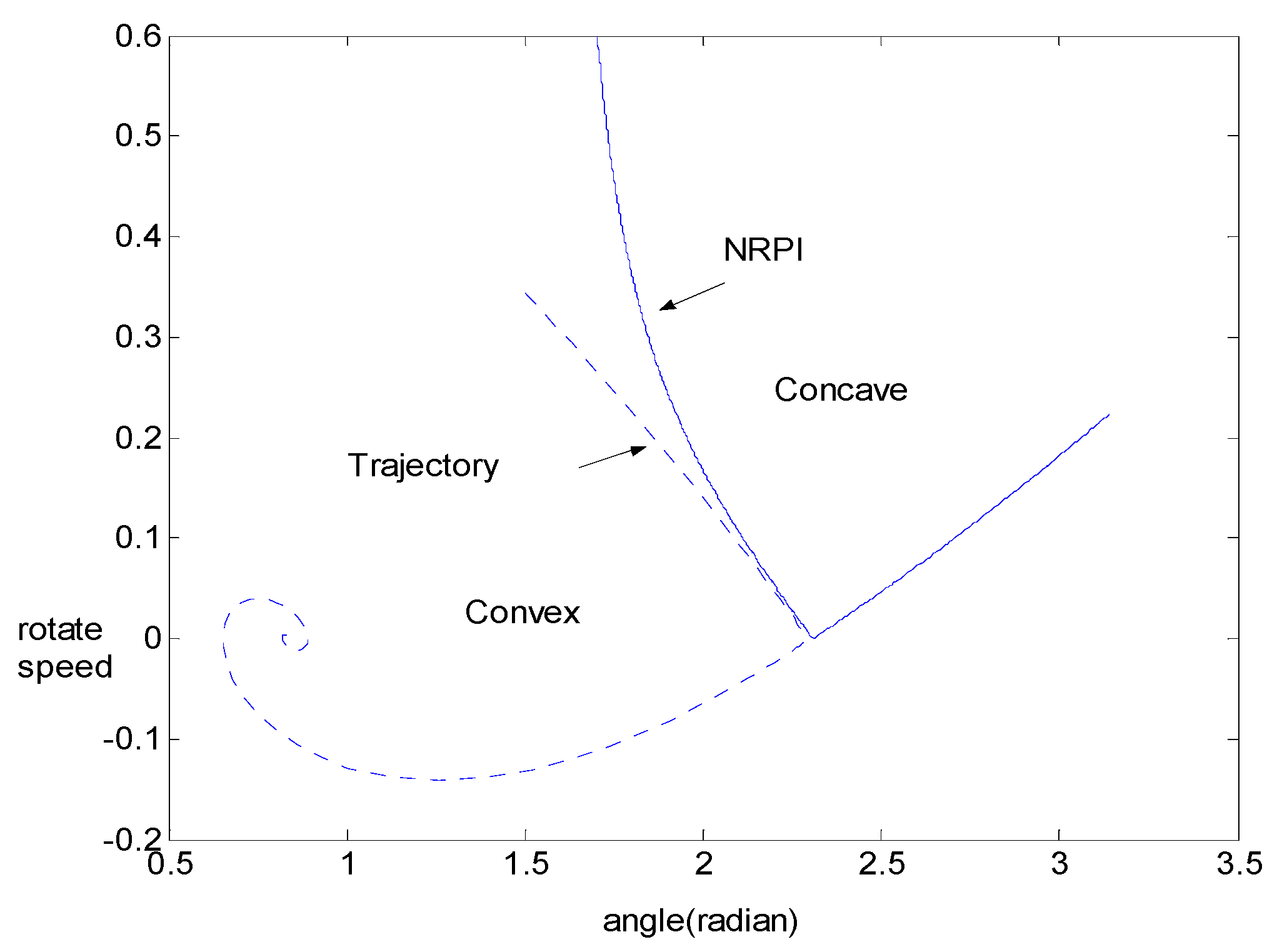
14]. Depending on the nature of the stability studied, Girgis has found that the characteristic shape (concave or convex) of a surface, on which a post-fault transient trajectory lies, can be used as an index for online instability detection [15]. The assumption is proved in a phase portrait, and an instability detection method is presented, which is independent of the network structure, system parameters and model because it only uses observation data. During the process of proof, a damping coefficient is considered in the system model to keep it more reasonable [16,17,18]. However, the discrete expression of the detection method in [18] requires differential calculations. The curve of the index looks ragged. For a stable situation after disturbances, it may cause some erroneous judgments.
This paper aims to introduce a real-time transient stability control system which employs the generator speed, power angle and unbalanced power to detect the system instability and develop a control strategy. In this paper, the system instability is detected by the characteristics concave or convex shape of the trajectory. Then, the control law is achieved based on the slope of the state plane trajectory, when the power system is unstable. Because the expected variables can be obtained from the trajectory information and the calculations are very simple, the control system can be realized in real time. The simulation indicates that the mentioned transient stability control system is fast, efficient, and realizable.

2. Instability Detection

2.1. Identification Method of Transient Instability for an Autonomous SMIB System

Previous research has found the geometric characteristics of the trajectory in a phase portrait can be employed to determine system instability through a great deal of simulation. It is found that stable trajectories are always concave with respect to the post-fault stable equilibrium point (SEP) and that unstable trajectories are convex with respect to the post-fault SEP immediately or a short time after the fault-clearing time as seen in Figure 1. The point at which the geometric characteristic of a system trajectory is convex, is defined as the no return point (NRP). All of these points (NRP) form of the interface that is defined as the no return point interface (NRPI).
Figure 1. System trajectories of a SMIB.
Energies 08 12381 g001
It should be particularly pointed out that the definition in this paper is different from the usual definition. As a rule, the point where a trajectory shifts to accelerated progress ( Δ P = 0 , δ = δ u e p , Δ P is the unbalanced power and δ u e p is the unstable equilibrium point) is defined as the NRP. The difference between both definitions is shown in Figure 1. Although Figure 1 is obtained for a specific set of system parameters, the characteristics of the system trajectory are typical of a single machine infinite bus (SMIB) system. Here, we use a SMIB system as an example to explain the foregoing concept. For the SMIB system, the system dynamics can be expressed as:
δ = ω 0 Δ ω Δ ω = [ P m P e m i sin δ D Δ ω ] / M
where δ and Δ ω are the generator angle and angular velocity with respect to a synchronous frame; D is the generator damping coefficient; M is the generator inertia; P m is the generator mechanical power input; and P e m i is the generator maximum electric power output.
On the basis of the definition of NRP, the tangent slope at any point on the trajectory of system Equation (1) is given as follows:
d Δ ω d t d δ d t = d Δ ω d δ = k ( δ , Δ ω ) = Δ P / ( M ω 0 Δ ω )
Consequently, the one-order derivative of the tangent slope at any point of the trajectory with respect to the generator angle (that is, the two-order derivative of the angular velocity with respect to the generator angle) can be expressed as:
l = d k d δ = k ( δ , Δ ω ) = [ P e m i cos ( δ ) D d Δ ω d δ ] M ω 0 Δ ω [ P m P e m i sin δ D Δ ω ] 2 / Δ ω ( M ω 0 Δ ω ) 2
On the ground of the definition of NRP, the point of system trajectory at which l = 0 is actually NRP. The interface (NRPI) that all of NRP constitute can be described as:
P e m i cos δ M ω 0 Δ ω D [ P m P e m i sin δ D ω ] [ P m P e m i sin δ D Δ ω ] 2 / Δ ω = 0
Figure 2 shows the NRPI divides the whole plane into two regions, i.e., a convex area and a concave area. In virtue of the mathematical definition, if l > 0 , we consider the geometrical characteristics of the post-fault trajectory is convex, while it is considered as concave if l < 0 .
We define the concavity and convexity of phase trajectory as follows:
(1)
The phase trajectory is convex if l Δ ω > 0 ;
(2)
The phase trajectory is concave if l Δ ω < 0 ;
(3)
The trajectory is on the inflexion point if l Δ ω = 0 .
In order to facilitate real-time computing, the unstable criterion can be expressed as:
τ = l Δ ω = d k d δ d δ d t 1 ω 0 = d k d t 1 ω 0 0
The discrete form of the index is given by:
τ ( i ) = Δ P ( i ) M Δ ω ( i ) Δ P ( i 1 ) M Δ ω ( i 1 )
Figure 2. Relationship of NRPI and the critical post-fault trajectory.
Energies 08 12381 g002
If τ is always less than zero, the system will be stable, while the system will lose synchronization immediately or a short time after the fault-clearing time if τ is larger than zero. The proposition has proved that the proposed index is a sufficient and necessary condition for instability detection of SMIB system.
It should be pointed out that the moment when the trajectory passes through the NRI is just the detection time. As shown in Figure 1, it can be found that the unstable trajectory is sure to pass through the NRI before it arriving at dynamic saddle point (DSP). Thus, by employing the characteristic concave or convex shapes of the trajectory one can easily and quickly identify the transient instability.

2.2. Identification Theory of Transient Instability for a Non-Autonomous SMIB System

The equations of an electromechanical transient process for non-autonomous SMIB system can be described as follows:
d δ d t = ω 0 Δ ω M d Δ ω d t = P m ( t ) P e ( t , δ ) = Δ P ( t , δ )
where the right function of the motion equation involves the variable of time, and thus Δ P ( t , δ ) doesn’t represent a strict sine function any more. As a consequence, the index τ greater than zero in a certain time can only indicate the instability of the autonomous system under that parameter condition, but not the non-autonomous system:
P e ( t i , δ ) = λ 0 ( t i ) λ 1 ( t i ) cos δ λ 2 ( t i ) sin δ Δ P ( t i , δ ) = P c ( t i ) λ 1 ( t i ) cos δ λ 2 ( t i ) sin δ
To fortify the accuracy of the detection, the index is established as follows. The feature index μ of trajectory in state-plane of unbalanced power and power angle is provided.
The feature index of the trajectory in state plane of unbalanced power and power angle is defined as:
d l d t | l = 0 = d 2 ( Δ P / M ) d δ 2
The discrete form is proposed as:
μ = Δ P ( i ) Δ P ( i 1 ) δ ( i ) δ ( i 1 ) Δ P ( i 1 ) Δ P ( i 2 ) δ ( i 1 ) δ ( i 2 ) > 0
The index means that the trajectory enters the convex region and does not return to the concave region in a short time. If the trajectory satisfies the index, the trajectory is unstable possibly.
Eventually, the instability criterion for a non-autonomous SMIB system can be described as:
τ > 0   &   μ > 0
The detection method launches when the power system is disturbed. If the maximum swing angle is less than 50°, the detection method automatically ends.

3. Control Method

There are many transient stability control measures, including generator shedding and load shedding [19,20]. In North America, generator shedding has been proved to be one of the most effective discrete supplementary control means for maintaining stability [21]. In this paper, generator shedding is mainly discussed too.

3.1. The Slope of the State-Plane Trajectory

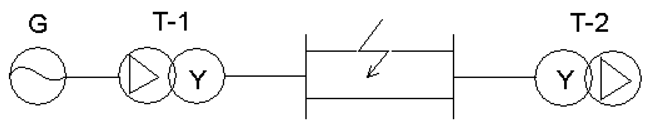
According to Equation (2), the expression of the slope is related to the unbalanced power which can be changed by generator shedding. It is supposed that the system returns to a stable state by generator shedding. If the value of the slope at control time is obtained, the corresponding generator shedding can be calculated by Equation (2). To obtain the value of the slope at control time, the characteristic of the slope is analyzed below. A single machine infinite bus system is shown in Figure 3.
Figure 3. The topology network of the SMIB system.
Energies 08 12381 g003
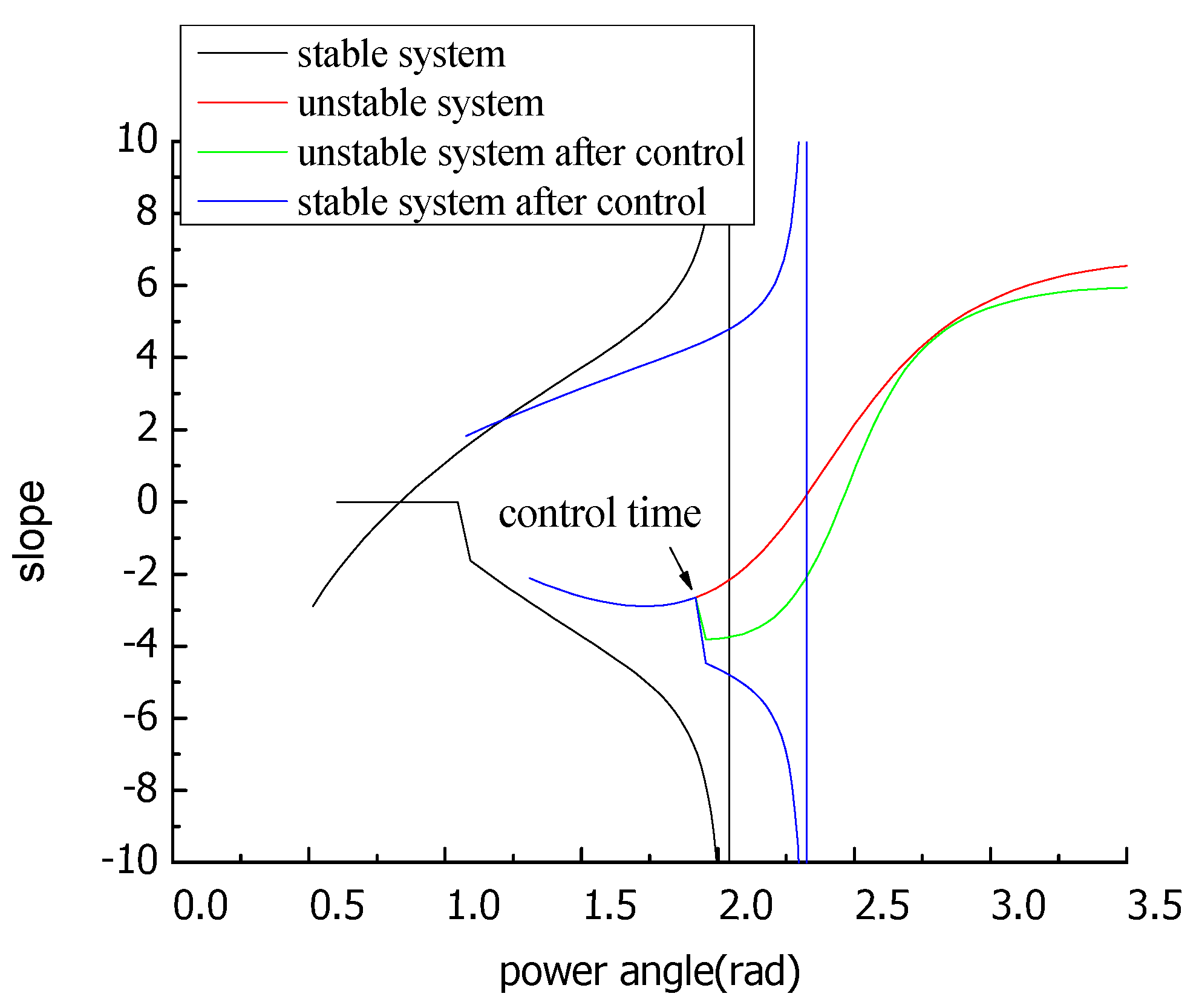
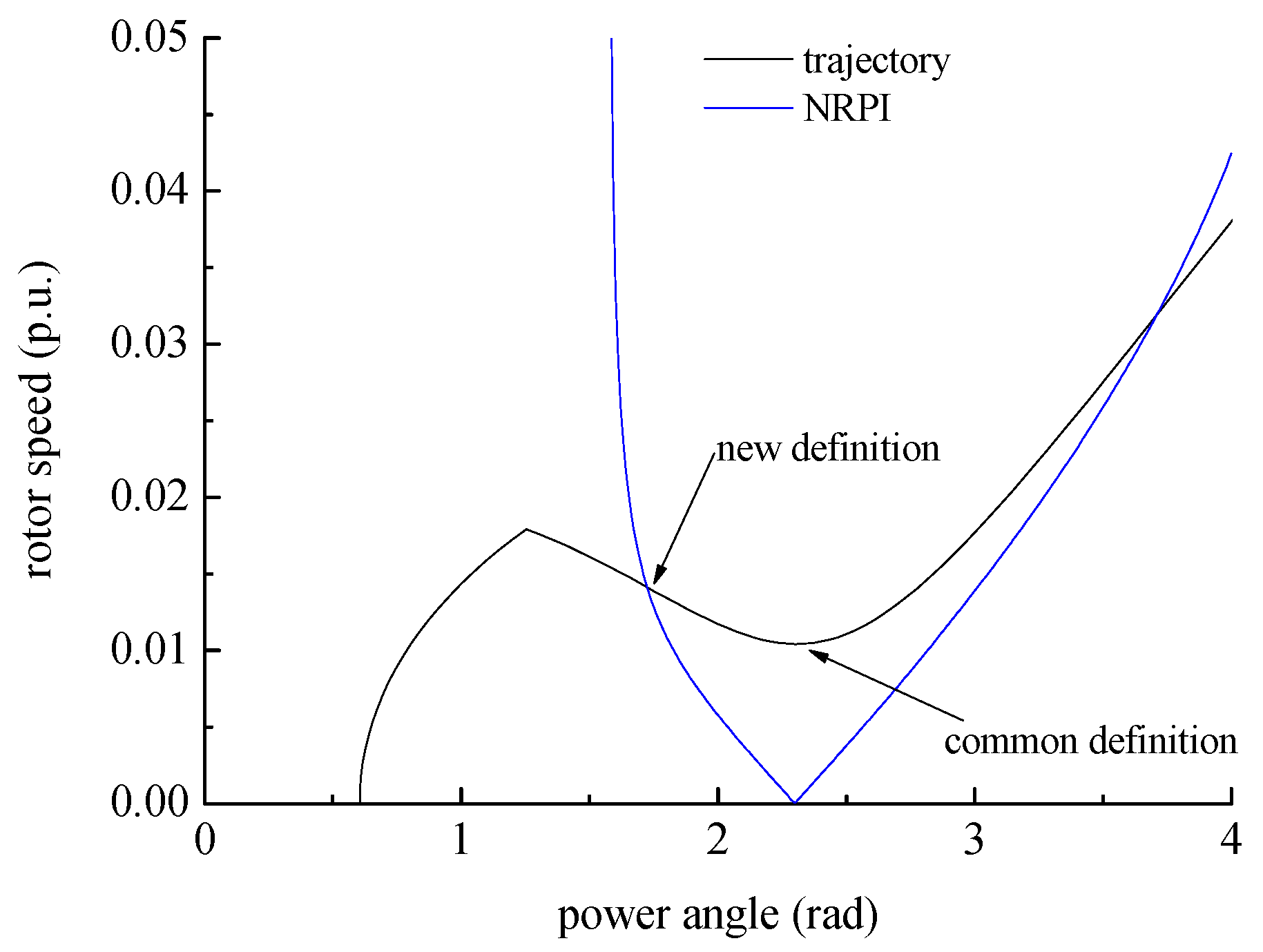
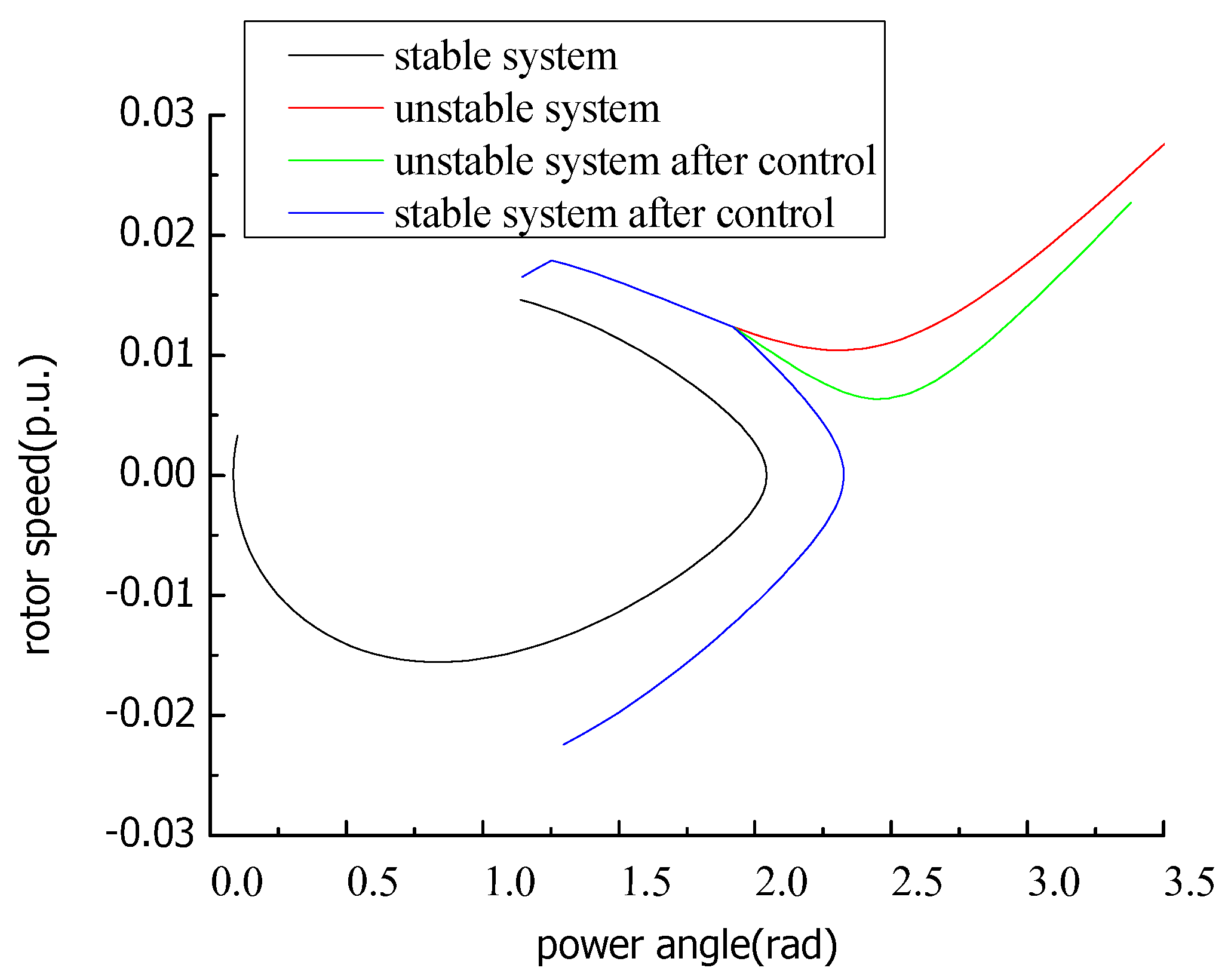
Under normal conditions, the system operates at a stable equilibrium point (SEP). The initial state of the generator is 0.812 rad, 0 rad/s. A three-phase grounding fault occurs on one of the two transmission lines, and the fault is cleared by switching off the line. The clearing time is 0.18 s (critical clearing time) and 0.22 s. When the system is unstable, different control quantities are taken. The trajectory of the state-plane and the slope of the trajectory are shown in Figure 4 and Figure 5.
For the black curve, the system is stable without control. The trajectory swings back at the far end point (FEP) which exists only in a stable system. The slope of the trajectory keeps decreasing with the mutation at the FEP.
For the red curve, the system is unstable without control. The slope begins to increase after the inflexion point and grows to zero at the dynamic saddle point (DSP).
For the green curve, the system is unstable with insufficient control. A sudden change of the slope is caused by the control at the control time. The larger the control quantity is, the greater the change of the slope at the control time is. However, the slope begins to increase at another inflexion point after control.
For the blue curve, the system is stable with enough control. The control causes a sudden reduction of the slope at the control time, and the slope keeps decreasing after the control with the mutation at the FEP. Apparently, the trajectory of the state-plane turns back at the unstable equilibrium point (UEP) by the minimum control quantity.
Figure 4. State-plane representation of speed and angle.
Energies 08 12381 g004
Figure 5. The slope over power angle.
Energies 08 12381 g005
The derivative of Equation (2) with respect to t is given by:
d k ( δ , ω ) d t = d k ( δ , ω ) d δ d δ d t = l   Δ ω = τ
A similar equation can be found in the detection algorithm mentioned in the previous article. Obviously the decrease of the slope indicates that the trajectory runs in the concave area, and the trajectory runs in the convex area after the slope begins to increase. If the control is appropriate, the system will return to a stable state and the slope of the trajectory will keep decreasing until it reaches FEP.

3.2. Calculation of Control Quantity for SMIB

To find the relationship between the slope and angular speed, integrating both sides of Equation (2) gives:
δ a δ b k ( δ , ω ) d δ = δ a δ b d Δ ω d δ d δ = Δ ω b Δ ω a
where δ a and δ b are the bounds of the integration; Δ ω a and Δ ω b are the angular speed corresponding to δ a and δ b . Let δ b be the power angle at the control time t a ; and then Δ ω a is the angular speed at t a . For stable state, Δ ω b is zero when δ b is the FEP. For unstable state, if Δ ω b can be zero by the control, the system will return from δ b to a stable state and δ b will be the FEP. Therefore Equation (13) can be written as:
δ a δ b k ( δ , ω ) d δ = Δ ω a
Therefore, the value of the slope at control time can be calculated by Equation (14), and the corresponding control quantity can be calculated by Equation (2). There are two unknowns δ b and k ( δ , ω ) in Equation (14). k ( δ , ω ) is related to the unbalanced power on the basis of Equation (2). δ b can be preset as the FEP as needed, but it must be no more than the UEP, so when δ b is acquired, k ( δ , ω ) can be calculated. If δ b is just the UEP, the corresponding control quantity is the minimum.

3.3. Approximation Method to Calculate Control Quantity

As can be seen from the trajectories in Figure 3, k ( δ , ω ) is nonlinear and changes corresponding to different control quantities at t a . Because of the nonlinear nature of k ( δ , ω ) , the value of k ( δ , ω ) at t a could not be acquired exactly. Therefore, an approximation method is presented to acquire the value of k ( δ , ω ) at t a . Employing a constant k instead of k ( δ , ω ) in Equation (14):
δ a δ b k d δ = k ( δ b δ a ) = Δ ω a
k = Δ ω a δ b δ a
Obviously, the angular speed and power angle at control time and the power angle at FEP are necessary to calculate k . Above all δ b must be preset less than or equal to UEP, then the system can be stable after control. Therefore, k ( δ , ω ) will keep decreasing after the control and the trajectory will return at δ b . Because that k ( δ , ω ) will keep decreasing after the control, k is surely less than the value of k ( δ , ω ) at control time. Hence, the control quantity calculated by k is a little bigger than actually needed.
For a SMIB system, suppose the ratio of generator shedding is λ , the relation of λ and k after control is as follows:
k = ( 1 λ ) P m P e a ( 1 λ ) M Δ ω a
λ = 1 P e a P m M Δ ω a k
where P e a is the generator output electrical power at t a . When k is obtained by Equation (16), the generator shedding ratio of SMIB system can be calculated by Equation (18).

3.4. Seeking for FEP

The parameters needed in calculation can be collected by WAMS except for FEP. Two methods to acquire the FEP are provided in this paper:
Method 1: In order to obtain the minimum control quantity, it is intended to slow down the angular speed to zero at UEP by the control. It can be supposed that the power equilibrium point of the system after control is the UEP. Generator electrical power can be written as Equation (19), and mechanical power is considered as a constant in a short time period. It is assumed that generator shedding has a corresponding change on mechanical power:
P e = P c ( t ) + λ 1 ( t ) sin ( δ ) + λ 2 ( t ) cos ( δ )
where P c ( t ) , λ 1 ( t ) , λ 2 ( t ) are parameters to be identified at t instant. P c ( t ) , λ 1 ( t ) , λ 2 ( t ) are considered as constant in a short time when no other operations occur. At t a instant, P c ( t a ) , λ 1 ( t a ) , λ 2 ( t a ) are calculated by the least square method, and then the electrical power can be acquired.
In order to seek for the UEP after the control, the control should be known at first. Therefore an iterative method can be employed as follows:
(1)
Obtain the prediction curve of the electrical power;
(2)
Preset zero to the generator shedding ratio and UPE: λ ( 0 ) = 0 , δ u ( 0 ) = 0 ;
(3)
Mechanical power decreases at the same ratio:
P m ( k ) = ( 1 λ ( k 1 ) ) P m ( k 1 )
(4)
Search for the power equilibrium point as δ b ( n ) ;
(5)
Acquire the λ ( k ) according to the δ b ( n ) ;
(6)
If | δ b ( n ) δ b ( n 1 ) | ε , complete the iterator; or return to step 3.
where ε is the convergence conditions; n is the number of the iterator.
Method 2: Preset a FEP as needed. On the basis of the operating requirement, the FEP, which must be less than or equal to the power equilibrium point, can be preset within the limits as needed.
Two control objectives are provided according to the way of acquiring the FEP: scheme one is the minimal cost to help restore the system to a stable state; scheme two is the minimal cost to limit the maximum angle.

3.5. Control Method for Multi-Machine System

Using the assumption made by [22] that the disturbed multi-machine system separates into two groups, leading group S and lagging group A, the partial center of angles, angular speed, mechanical power and electrical power of the two-machine power system are shown as follows:
δ s = i S M i δ i i S M i      δ a = i A M i δ i i A M i
Δ ω s = i S M i Δ ω i i S M i      Δ ω a = i A M i Δ ω i i A M i
P m s = i S P m i      P m a = i A P m i P e s = i S P e i      P e a = i A P e i
Further, the two-machine power system can be equivalent to the SMIB system:
δ = δ s δ a
Δ ω = Δ ω s Δ ω a
Δ P = P M P E
where
M T = i = 1 n M i , M = M s M a M T , P M = M a P m s M s P m a M T , P E = M a P e s M s P e a M T .
According to the calculation method applied to SMIB equivalent system, the expected slope k of SMIB equivalent system can be acquired. Transform the expected slope to control quantity:
Δ P m s = M s ( k k ) ω 0 ( Δ ω s Δ ω a )
where k is the original slope before control.

4. Simulation Result

4.1. SMIB System

The SMIB system as shown in Figure 3 is employed to illustrate the algorithm. Under normal conditions, the system operates at a stable equilibrium point. A three-phase grounding fault occurs on line L2, and the fault is cleared by switching off the line. The clear time differ from 0.17 s (critical clearing time) to 0.22 s. The system parameters are shown in Table 1.
Table 1. The parameters of the SMIB system.
ComponentParameters
The initial state ω 0 = 2 π f , f = 50 Hz , δ 0 = 34.49
The generator P m = 120 MW , T j = 6 s , x d = 1.83 p.u. , x q = 1.83 p.u. , x d = 0.3 p.u. , x q = 1.83 p.u. , x q = 0.25 p.u. , x d = 0.25 p.u.
The transmission line x 1 = x 2 = 0.486 Ω/km ,   x 0 = 4 x 1
It is needed to point out that the simulation just acquires the power angle, angular speed, mechanical power, electrical power, inertia constant of the generator without other information, which can be acquired on-line. When the sampling time interval is 10 ms, the detection results based on the instability criterion mentioned above are shown in Table 2.
Table 2. The transient stability detection results by 100 Hz sample frequency.
The Moment of Fault-ClearingSimulation ResultsDetection ResultsThe Moment of Instability DetectedThe Angle of Instability Detected
0.17 sStableStable\\
0.18 sStableStable\\
0.187 sStableStable\\
0.188 sUnstableUnstable0.56 s121.9°
0.19 sUnstableUnstable0.46 s114.9°
0.20 sUnstableUnstable0.37 s106.2°
0.21 sUnstableUnstable0.34 s102.9°
0.22 sUnstableUnstable0.33 s102.8°
When the sampling time interval is 20 ms, the detection results based on the instability criterion mentioned above are shown in Table 3.
Table 3. The transient stability detection results by 50 Hz sample frequency.
The Moment of Fault-ClearingSimulation ResultsThe Moment of Instability DetectedThe Angle of Instability DetectedThe Moment of Angle Reach the Threshold of 180°
0.17 sStableStable--
0.18 sStableStable--
0.187 sStableStable--
0.188 sUnstable0.56 s121.9°1.44 s
0.19 sUnstable0.46 s114.9°1.14 s
0.20 sUnstable0.38 s108.5°0.86 s
0.21 sUnstable0.34 s102.9°0.76 s
0.22 sUnstable0.34 s105.6°0.68 s
The results in Table 2 and Table 3 show that the instability criterion mentioned in this paper can distinguish unstable cases and stable cases correctly and rapidly. Even the critical cases of which the difference of fault-clearing time is only 1 ms can be rightly detected. The accuracy of the detection result is not influenced by the sample frequency. From the results in Table 3, the angles of instability detected vary from 102.9° to 121.9°, which are much less than 180°. Further, the detection moment of the method proposed in this paper is much earlier than it of the threshold of 180°, which can provide adequate time for implementation of control measures.
It is necessary to take some control actions when the system is detected as unstable. Two control objectives are provided by the way to acquire the FEP: scheme one is the minimal cost to help the system restore to stable state; scheme two is the minimal cost to limit the maximum angle.
When the system is unstable, the control quantity is calculated by scheme one. The results are shown in Table 4. The minimum control quantity calculated by scheme one is close to and a little bigger than the real minimum control quantity. The control quantity calculated by this paper is effective and conservative as expected. In addition, the conservative algorithm is helpful for the recovery of the power system.
The same condition introduced above, control quantity is calculated by scheme two, and the preset FEP is 130°.The result is shown in Table 5. The FEP after control is closed to and less than 130° as expected. It means that the scheme two intended to limit the FEP of the power system is effective. Transient stability margin is directly reflected in the angle swing range. The method can be applied to improve the transient stability margin when the power system suffers large disturbance.
Table 4. Calculated minimum control compare to the real minimum control.
Fault-Clearing TimeDistinction TimeCalculated Minimum Control Quantity (%)Real Minimum Control Quantity (%)
0.18 sNone (stable)None (stable)None (stable)
0.19 s0.46 s5.614.55
0.20 s0.37 s14.113.5
0.21 s0.34 s22.420.6
0.22 s0.33 s30.128.4
Table 5. Calculated minimum control by limiting the maximum angle.
Fault-Clearing TimeDistinction TimeCalculated Controlled Quantity (%)Real FEP after Control
0.18 sNone (stable)None (stable)None (stable)
0.19 s0.46 s8.91129.1°
0.20 s0.37 s18.6126.8°
0.21 s0.34 s22.5128.1°
0.22 s0.33 s35.6128.8°

4.2. IEEE 39-Bus System

The IEEE 39-bus system shown in Figure 6 is employed to illustrate the algorithm. Two control objectives are provided according to the way of acquiring the FEP: scheme one is the minimal cost to help the system restore to stable state; scheme two is the minimal cost to limit the maximum angle.
Figure 6. The diagram of IEEE 10-unit 39-bus power system.
Energies 08 12381 g006
A three-phase grounding fault occurs on the transmission line between bus 4 and bus 14 and the fault duration is 0.4 s. The power angle curves are shown in Figure 7.
Figure 7. Multi-machine swing curves after fault.
Energies 08 12381 g007
The results of the closed loop control system are shown in Table 6.
Table 6. Results of the control system.
FaultA Three-Phase Grounding Fault Occurs on the Line between Bus 4 and Bus 14
Fault duration0.23 s
Detection time0.41 s
Detection angle126.5904°
Control objectivescheme onescheme two (145°)
Control law (MW)G31 (439)G31 (521)
FEP after control148.0°144.8°
The power angle curves after scheme one are shown in Figure 8. It can be seen that both scheme one and scheme two quickly dampen the system oscillation and keep the system stable. The cost of scheme one is 439 MW, and the FEP after control is 148.0°. The cost of scheme two is 521 MW, and the FEP is 144.8° within the limit.
Figure 8. Power angle curves of scheme one.
Energies 08 12381 g008

5. Conclusions

In conclusion, the detection method and the control method deduced in this paper just use real-time information rather than the information of system models, parameters and disturbances to deal with the transient instability problem. As a result, the control system could be applicable in real time. The detection technique can identify instability accurately and quickly. Based on the tangent slope of the state plane trajectory, a new control method proposed in this paper forms a transient stability control system with the detection method. Two control objectives which are successfully tested in the simulations are provided based on the method of acquiring FEP in this paper. The simulation results in SMIB system and IEEE 39-bus system indicate the effectiveness of the proposed transient stability control system.

Author Contributions

Zhiguo Hao and Baohui Zhang checked and discussed the simulation results. Huaiyuan Wang confirmed the series of simulation parameters and arranged and organized the entire simulation process. Baohui Zhang and Zhiguo Hao made many useful comments and simulation suggestions. In addition, all authors reviewed the manuscript.

Conflicts of Interest

The authors declare no conflict of interest.

References

  1. Anjan, B. Application of direct method to transient stability analysis of power system. IEEE Trans. Power Appar. Syst. 1984, 103, 1629–1635. [Google Scholar]
  2. Ota, H.; Kitayama, Y.; Ito, H.; Fukushima, N.; Omata, K.; Morita, K.; Kokai, Y. Development of transient stability control system (TSC system) based on on-line stability calculation. IEEE Trans. Power Syst. 1996, 11, 1463–1472. [Google Scholar] [CrossRef]
  3. Mahmud, M.A.; Pota, H.R.; Aldeen, M.; Hossain, M. Partial feedback linearizing excitation controller for multimachine power systems to improve transient stability. IEEE Trans. Power Syst. 2014, 29, 561–571. [Google Scholar] [CrossRef]
  4. Beerten, J.; Cole, S.; Belmans, R. Modeling of multi-terminal VSC HVDC systems with distributed DC voltage control. IEEE Trans. Power Syst. 2014, 29, 34–42. [Google Scholar] [CrossRef]
  5. Wang, L.; Morison, K. Implementation of online security assessment. IEEE Power Energy Mag. 2006, 4, 46–59. [Google Scholar] [CrossRef]
  6. Madani, V.; Novosel, D.; Horowitz, S.; Adamiak, M.; Amantegui, J.; Karlsson, D.; Imai, S.; Apostolov, A. IEEE PSRC report on global industry experiences with system integrity protection schemes(SIPS). IEEE Trans. Power Deliv. 2010, 25, 2143–2155. [Google Scholar] [CrossRef]
  7. Kim, S.; Overbye, T.J. Optimal subinterval selection approach for power system transient stability simulation. Energies 2015, 8, 11871–11882. [Google Scholar] [CrossRef]
  8. Vega, R.; Glavic, M.; Ernst, D. Transient stability emergency control combining open-loop and closed-loop techniques. In Proceeding of the IEEE Power Engineering Society General Meeting, Toronto, ON, Canada, 13–17 July 2003; Volume 4, pp. 13–17.
  9. Pai, A. Energy Function Analysis for Power System Stability; Springer Science & Business Media: Heidelberg, Germany, 2012. [Google Scholar]
  10. Ruiz-Vega, D.; Pavella, M. A comprehensive approach to transient stability control. I. Near optimal preventive control. IEEE Trans. Power Syst. 2003, 18, 1446–1453. [Google Scholar] [CrossRef]
  11. Xue, Y.; Wehenkel, L.; Belhomme, R.; Rousseaux, P.; Pavella, M.; Euxibie, E.; Heilbronn, B.; Lesigne, J.F. Extended equal area criterion revisited (EHV power systems). IEEE Trans. Power Syst. 1992, 7, 1012–1022. [Google Scholar] [CrossRef]
  12. Pavella, M.; Ernst, D.; Ruiz-Vega, D. Transient Stability of Power Systems: A Unified Approach to Assessment and Control; Kluwer: Boston, MA, USA, 2000. [Google Scholar]
  13. Jin, T.; Chu, F.; Ling, C.; Nzongo, D. A robust WLS power system state estimation method integrating a wide-area measurement system and SCADA technology. Energies 2015, 8, 2769–2787. [Google Scholar] [CrossRef]
  14. Wang, L.; Girgis, A.A. A new method for power system transient instability detection. IEEE Trans. Power Deliv. 1997, 12, 1082–1088. [Google Scholar] [CrossRef]
  15. Xie, H.; Zhang, B.; Yu, G.; Li, Y.; Li, P.; Zhou, D.; Yao, F. Power systems transient stability detection theory based on characteristic concave or convex of trajectory. Proc. CSEE 2006, 26, 38–42. [Google Scholar]
  16. Xie, H.; Zhang, B. Power system transient stability detection based on characteristic concave or convex of trajectory. In Proceedings of the IEEE Transmission and Distribution Conference & Exhibition: Asia and Pacific, Dalian, China, 15–18 August 2005.
  17. Zhang, B.; Yang, S.; Wang, H. Closed-loop control of power system transient stability (1): Transient instability detection principle of simple power system. Electr. Power Autom. Equip. 2014, 8, 1–6. [Google Scholar]
  18. Zhang, B.; Yang, S.; Wang, H. Closed-loop control of power system transient stability (3): Initiation criterion of transient stability closed-loop control based on predicted response of power system. Electr. Power Autom. Equip. 2014, 10, 1–6. [Google Scholar]
  19. Shao, H.; Lin, Z.; Norris, S.; Bialek, J. Application of emergency-single machine equivalent method for cascading outages. In Proceedings of the Power Systems Computation Conference (PSCC), Wrocław, Poland, 18–22 August 2014; pp. 1–6.
  20. Jiang, Q.; Wang, Y.; Geng, G. A parallel reduced-space interior point method with orthogonal collocation for first-swing stability constrained emergency control. IEEE Trans. Power Syst. 2014, 29, 84–92. [Google Scholar] [CrossRef]
  21. Fouad, A.A.; Ghafurian, A.; Nodehi, K.; Mansour, Y. Calculation of generation-shedding requirements of the BC hydro system using transient energy functions. IEEE Trans. Power Syst. 1986, 1, 17–23. [Google Scholar] [CrossRef]
  22. Xue, Y.; van Custem, T.; Pavella, M. Extended equal area criterion justifications, generalizations, applications. IEEE Trans. Power Syst. 1989, 4, 44–52. [Google Scholar] [CrossRef]

