
Governor Design for a Hydropower Plant with an Upstream Surge Tank by GA-Based Fuzzy Reduced-Order Sliding Mode

Abstract
:1. Introduction

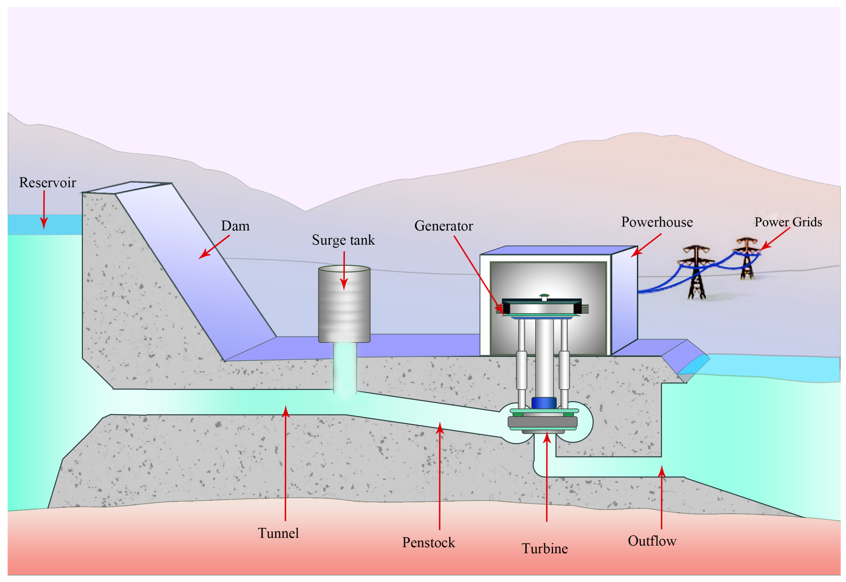
2. Dynamics of a Hydropower Plant with an Upstream Surge Tank
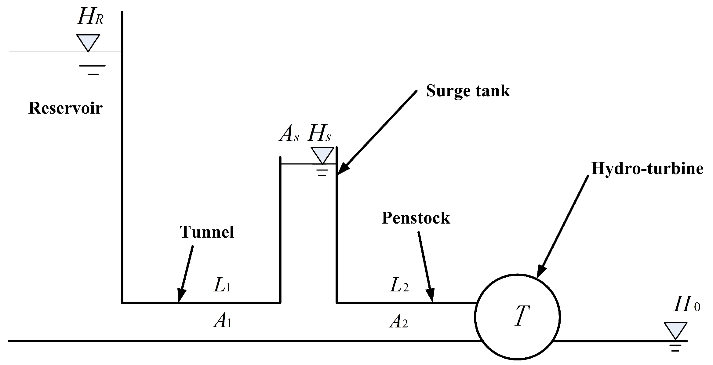
2.1. Water Hammer
2.2. Tunnel
2.3. Penstock
2.4. Surge Tank
2.5. Wicket Gate and Servomechanism
2.6. Hydro-Turbine
2.7. Generator and Grid

3. Control Design
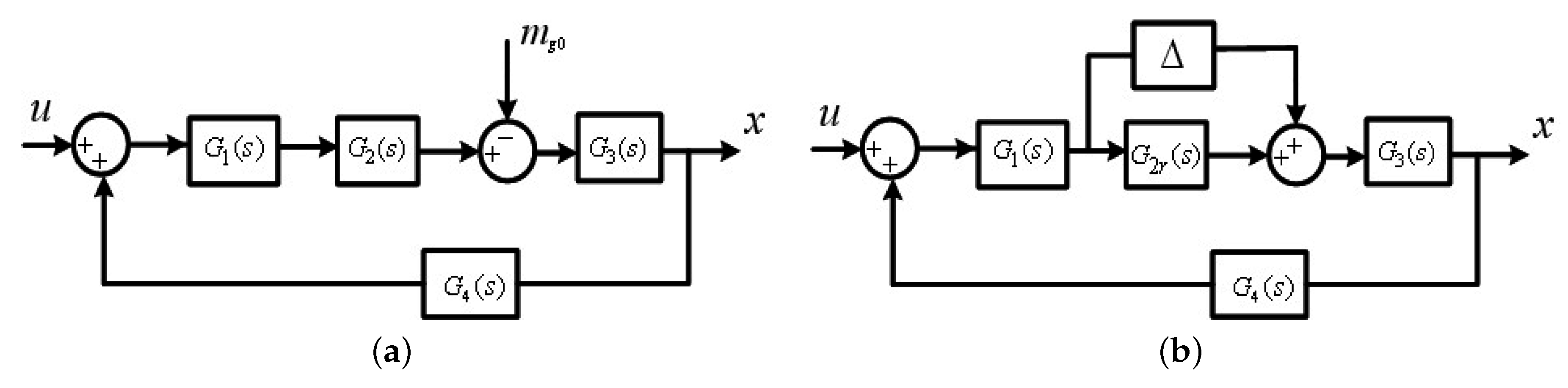
3.1. Design of the Reduced-Order Sliding Mode Controller
3.2. GA-Based Parameter Optimization
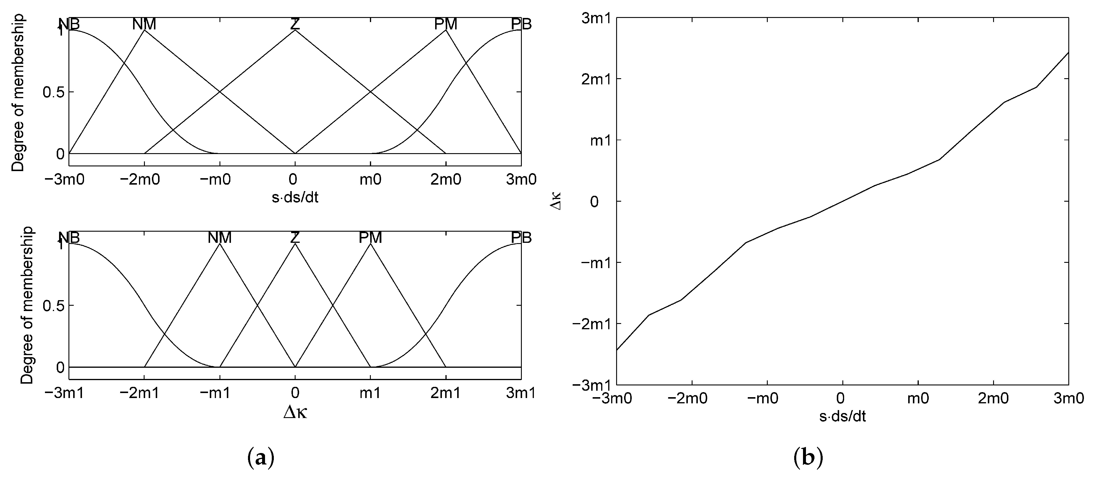
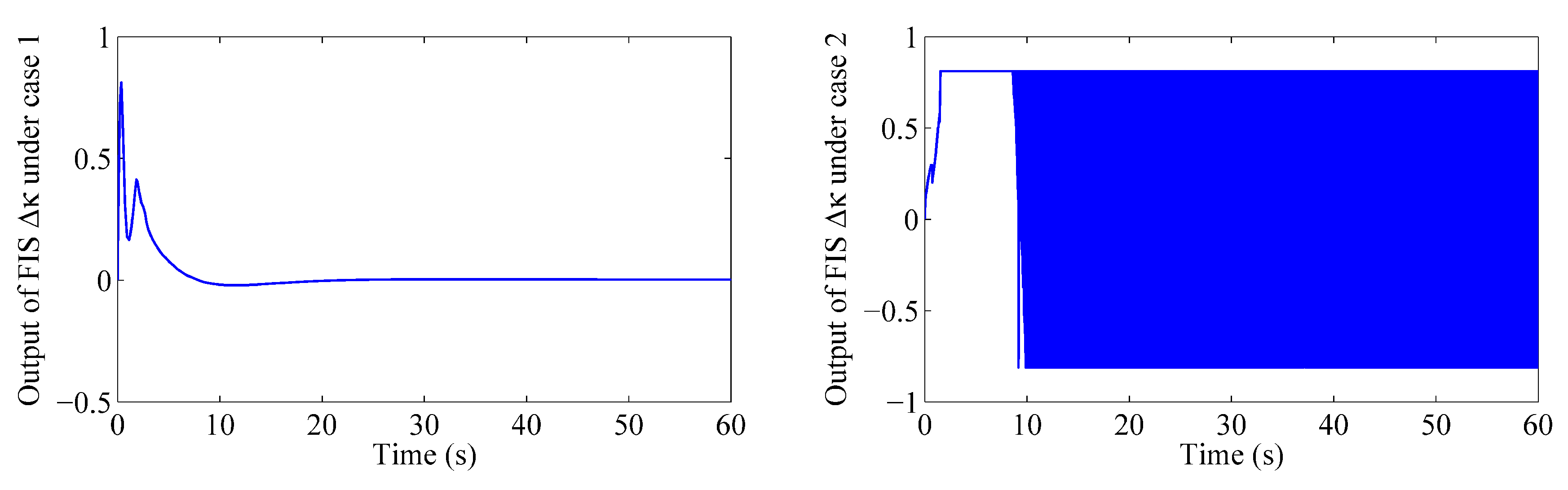
3.3. Design of the Fuzzy Inference System
- If is PB, then Δκ is PB.
- If is PM, then Δκ is PM.
- If is Z, then Δκ is Z.
- If is NM, then Δκ is NM.
- If is NB, then Δκ is NB.
4. Simulation Results

| Coefficients | ex | ey | eh | eqx | eqy | eqh | eg |
|---|---|---|---|---|---|---|---|
| Case 1 | −1.000 | 1.000 | 1.500 | 0.000 | 1.000 | 0.500 | 0.210 |
| Case 2 | −0.260 | 0.322 | 0.722 | 0.000 | 0.573 | 0.325 | 0.210 |
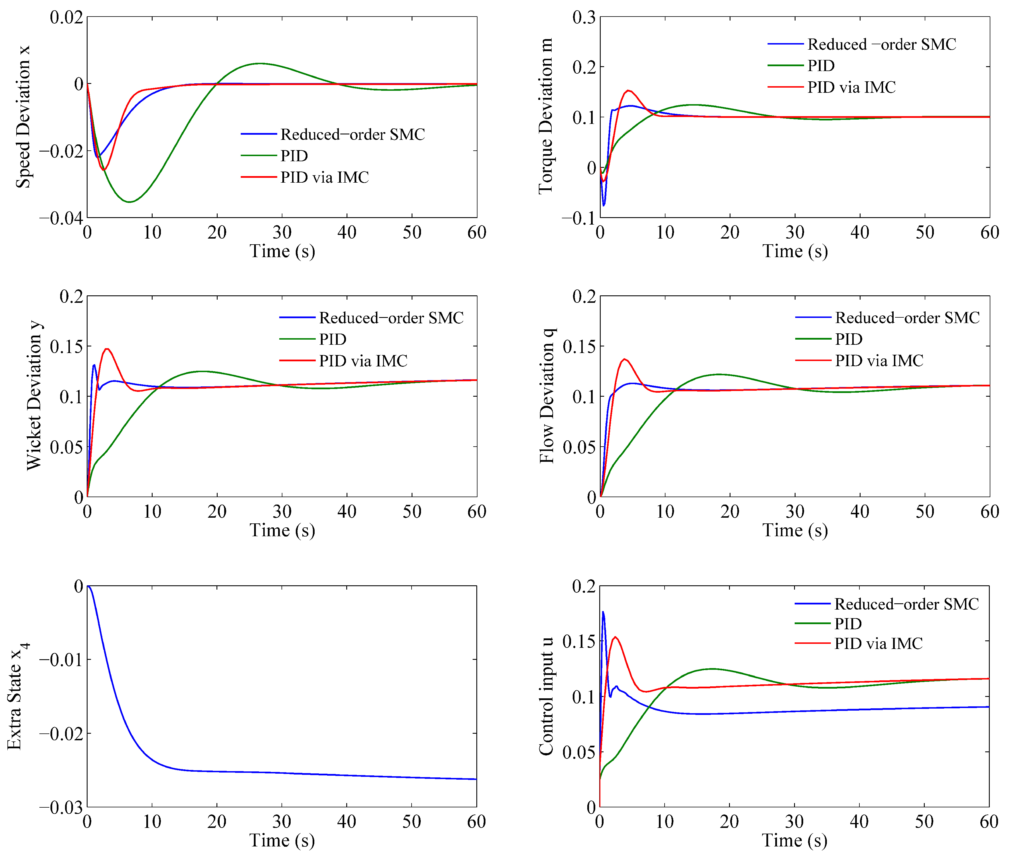
4.1. Load Rejection

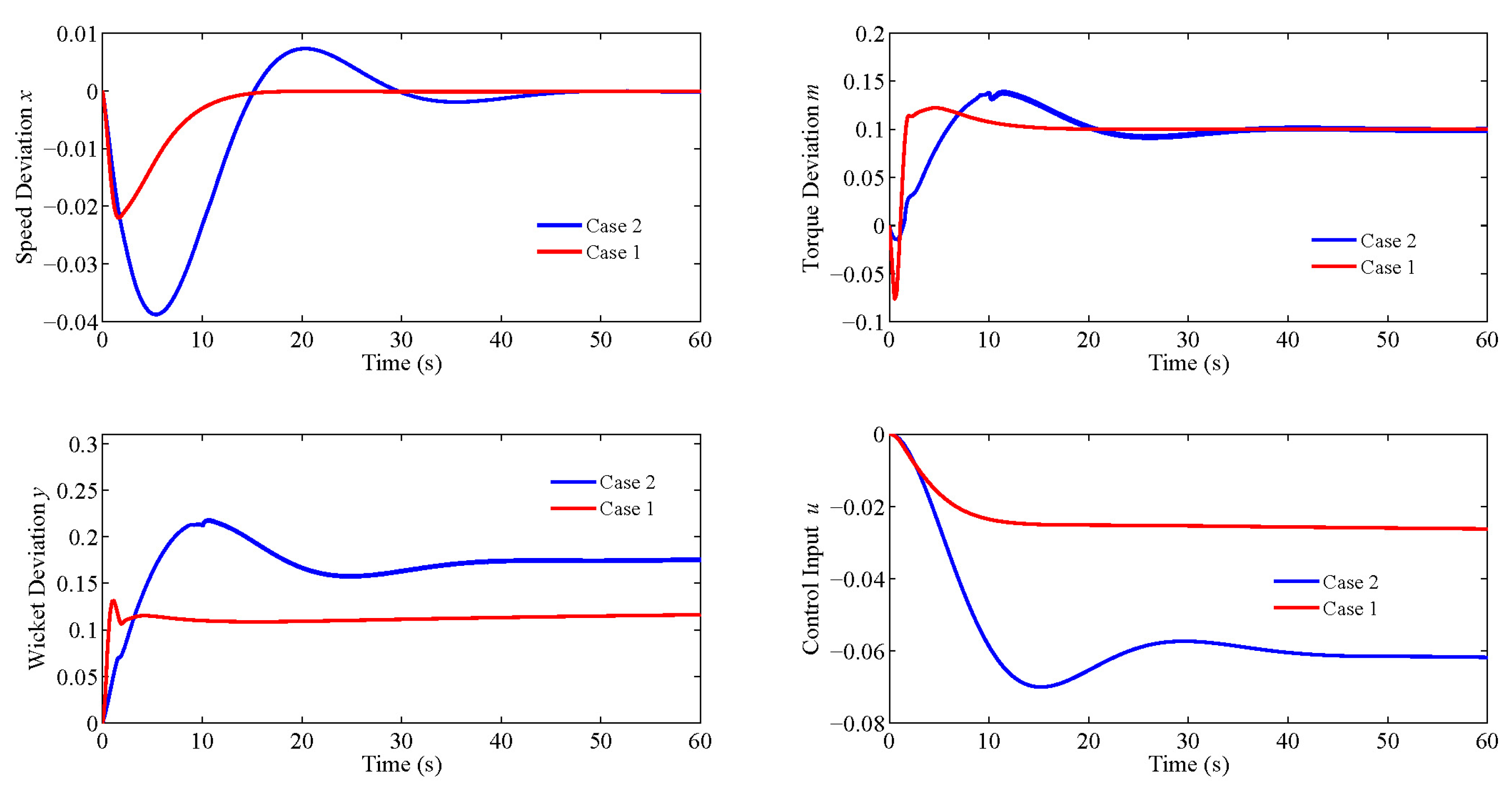
4.2. Robustness Testing


5. Conclusions
Acknowledgments
Author Contributions
Conflicts of Interest
Appendix
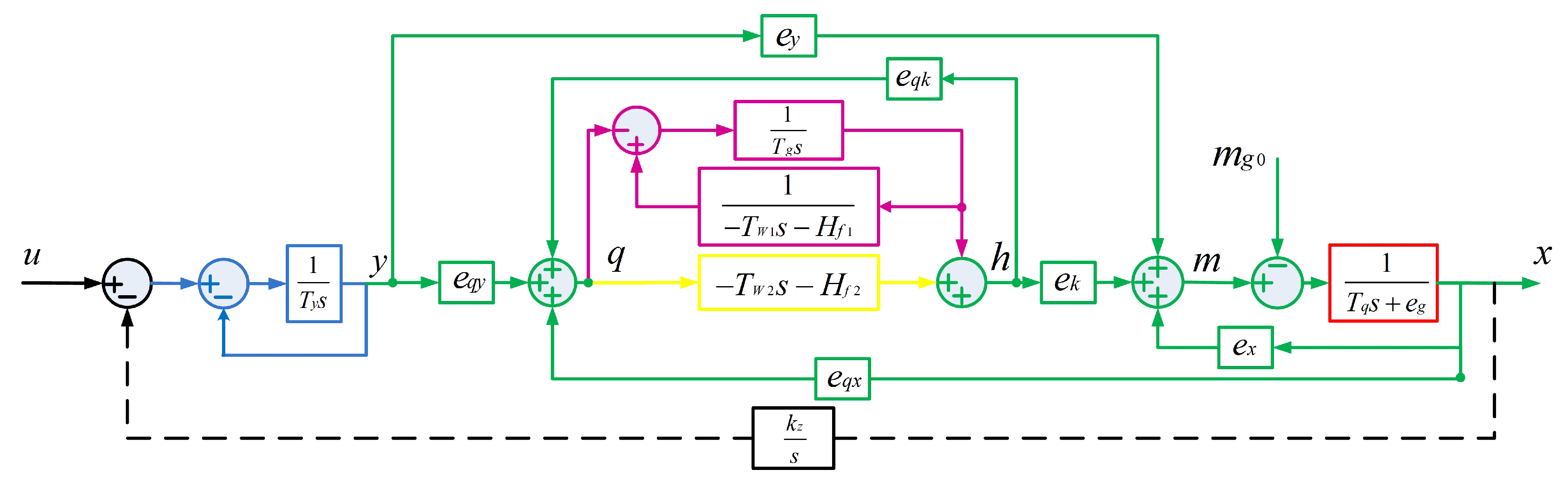
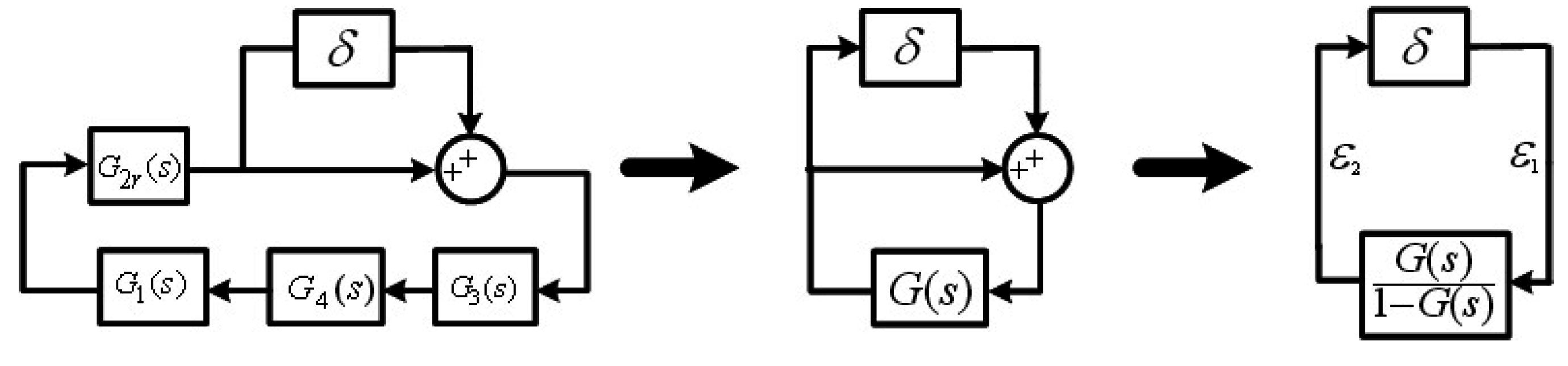
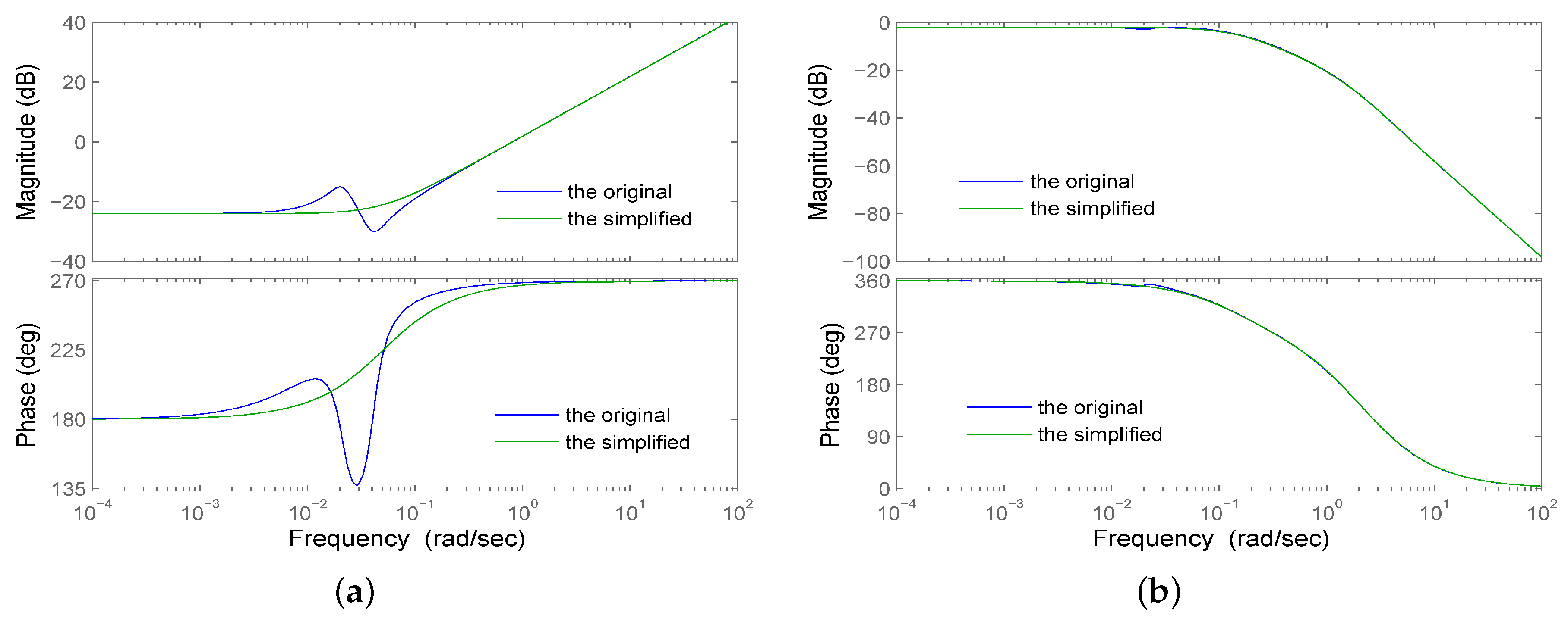
Appendix A. Reduced-Order Model
Appendix B. Proof of Theorem 3.1


References
- Cuellar, A.D.; Herzog, H. A path forward for low carbon power from biomass. Energies 2015, 8, 1701–1715. [Google Scholar] [CrossRef]
- Rahi, O.P.; Chandel, A.K. Refurbishment and uprating of hydro power plants—A literature review. Renew. Sustain. Energy Rev. 2015, 48, 726–737. [Google Scholar] [CrossRef]
- Nagode, K.; Skrjanc, I. Modelling and internal fuzzy model power control of a Francis water turbine. Energies 2014, 7, 874–889. [Google Scholar] [CrossRef]
- Kishor, N.; Saini, R.P.; Singh, S.P. A review on hydropower plant models and control. Renew. Sustain. Energy Rev. 2007, 11, 776–796. [Google Scholar] [CrossRef]
- Fang, H.Q.; Chen, L.; Dlakavu, N.; Shen, Z.Y. Basic modeling and simulation tool for analysis of hydraulic transients in hydroelectric power plants. IEEE Trans. Energy Convers. 2008, 23, 834–841. [Google Scholar] [CrossRef]
- Natarajan, K. Robust PID controller design for hydroturbines. IEEE Trans. Energy Convers. 2005, 20, 661–667. [Google Scholar] [CrossRef]
- Jiang, C.W.; Ma, Y.C.; Wang, C.M. PID controller parameters optimization of hydro-turbine governing systems using deterministic-chaotic-mutation evolutionary programming (DCMEP). Energy Convers. Manag. 2006, 47, 1222–1230. [Google Scholar] [CrossRef]
- Fang, H.; Chen, L.; Shen, Z. Application of an improved PSO algorithm to optimal tuning of PID gains for water turbine governor. Energy Convers. Manag. 2011, 52, 1763–1770. [Google Scholar] [CrossRef]
- Husek, P. PID controller design for hydraulic turbine based on sensitivity margin specifications. Int. J. Electr. Power Energy Syst. 2014, 55, 460–466. [Google Scholar] [CrossRef]
- Jones, D.; Mansoor, S. Predictive feedforward control for a hydroelectric plant. IEEE Trans. Control Syst. Technol. 2004, 12, 956–965. [Google Scholar] [CrossRef]
- Kishor, N.; Singh, S.P. Simulated response of NN based identification and predictive control of hydro plant. Expert Syst. Appl. 2007, 32, 233–244. [Google Scholar] [CrossRef]
- Mahmoud, M.; Dutton, K.; Denman, M. Design and simulation of a nonlinear fuzzy controller for a hydropower plant. Electr. Power Syst. Res. 2005, 73, 87–99. [Google Scholar] [CrossRef]
- Jiang, J. Design of an optimal robust governor for hydraulic turbine generating units. IEEE Trans. Energy Convers. 1995, 10, 188–194. [Google Scholar] [CrossRef]
- Qian, D.; Yi, J. 1 adaptive governor design for hydro-turbines. ICIC Express Lett. Part B Appl. 2013, 3, 1171–1177. [Google Scholar]
- Ding, X.; Sinha, A. Sliding mode/H∞ control of a hydro-power plant. In Proceedings of the American Control Conference, San Francisco, CA, USA, 29 June–1 July 2011.
- Salhi, I.; Doubabi, S.; Essounbouli, N.; Hamzaoui, A. Application of multi-model control with fuzzy switching to a micro hydro-electrical power plant. Renew. Energy 2010, 35, 2071–2079. [Google Scholar] [CrossRef]
- Qian, D.W.; Zhao, D.B.; Yi, J.Q.; Liu, X.J. Neural sliding-mode load frequency controller design of power systems. Neural Comput. Appl. 2013, 22, 279–286. [Google Scholar] [CrossRef]
- Erschler, J.; Roubellat, F.; Vernhes, J.P. Automation of a hydroelectric power station using variable-structure control systems. Automatica 1974, 10, 31–36. [Google Scholar] [CrossRef]
- Ye, L.Q.; Wei, S.P.; Xu, H.B.; Malik, O.P.; Hope, G.S. Variable structure and time-varying parameter control for hydroelectric generating unit. IEEE Trans. Energy Convers. 1989, 4, 293–299. [Google Scholar]
- Jing, L.; Ye, L.Q.; Malik, O.P.; Zeng, Y. An intelligent discontinuous control strategy for hydroelectric generating unit. IEEE Trans. Energy Convers. 1998, 13, 84–89. [Google Scholar] [CrossRef]
- Hydraulic Turbine and Turbine Control Models for System Dynamic Studies. Available online: http://ieeexplore.ieee.org/xpl/articleDetails.jsp?tp=&arnumber=141700 (accessed on 23 November 2015).
- Qian, D.; Yi, J.; Liu, X. Design of reduced order sliding mode governor for hydro-turbines. In Proceedings of the American Control Conference, San Francisco, CA, USA, 29 June–1 July 2011.
- Kendir, T.E.; Ozdamar, A. Numerical and experimental investigation of optimum surge tank forms in hydroelectric power plants. Renew. Energy 2013, 60, 323–331. [Google Scholar] [CrossRef]
- Chen, D.; Ding, C.; Ma, X.; Yuan, P.; Ba, D. Nonlinear dynamical analysis of hydro-turbine governing system with a surge tank. Appl. Math. Model. 2013, 37, 7611–7623. [Google Scholar] [CrossRef]
- Ghidaoui, M.S.; Zhao, M.; McInnis, D.A.; Axworthy, D.H.; McInnis, D.A. A review of water hammer theory and practice. Appl. Mech. Rev. 2005, 58, 49–76. [Google Scholar] [CrossRef]
- Sanathanan, C.K. Accurate Low Order Model for Hydraulic Turbine-Penstock. IEEE Trans. Energy Convers. 1987, 2, 196–200. [Google Scholar] [CrossRef]
- Doan, R.E.; Natarajan, K. Modeling and control design for governing hydroelectric turbines with leaky Wicket gates. IEEE Trans. Energy Convers. 2004, 19, 449–455. [Google Scholar] [CrossRef]
- Tan, W. Unified tuning of PID load frequency controller for power systems via IMC. IEEE Trans. Power Syst. 2010, 25, 341–350. [Google Scholar] [CrossRef]
- Cheng, L.; Hou, Z.G.; Lin, Y.Z.; Tan, M.; Zhang, W.C.; Wu, F.X. Recurrent neural network for non-smooth convex optimization problems with application to the identification of genetic regulatory networks. IEEE Trans. Neural Netw. 2011, 22, 714–726. [Google Scholar] [CrossRef] [PubMed]
- Tan, W. Analysis and design of a double two-degree-of-freedom control scheme. ISA Trans. 2010, 49, 311–317. [Google Scholar] [CrossRef] [PubMed]
- Streeter, V.L.; Wylie, B.E. Fluid Mechanics; McGraw-Hill: New York, NY, USA, 1979. [Google Scholar]
- Khalil, H.K. Nonlinear Systems, 3rd ed.; Prentice Hall: Upper Saddle River, NJ, USA, 2002. [Google Scholar]
© 2015 by the authors; licensee MDPI, Basel, Switzerland. This article is an open access article distributed under the terms and conditions of the Creative Commons by Attribution (CC-BY) license (http://creativecommons.org/licenses/by/4.0/).
Share and Cite
Xu, C.; Qian, D. Governor Design for a Hydropower Plant with an Upstream Surge Tank by GA-Based Fuzzy Reduced-Order Sliding Mode. Energies 2015, 8, 13442-13457. https://doi.org/10.3390/en81212376
Xu C, Qian D. Governor Design for a Hydropower Plant with an Upstream Surge Tank by GA-Based Fuzzy Reduced-Order Sliding Mode. Energies. 2015; 8(12):13442-13457. https://doi.org/10.3390/en81212376
Chicago/Turabian StyleXu, Chang, and Dianwei Qian. 2015. "Governor Design for a Hydropower Plant with an Upstream Surge Tank by GA-Based Fuzzy Reduced-Order Sliding Mode" Energies 8, no. 12: 13442-13457. https://doi.org/10.3390/en81212376