Overview of Modelling and Advanced Control Strategies for Wind Turbine Systems

Abstract

The motivation for this paper comes from a real need to have an overview of the challenges of modelling and control for very demanding systems, such as wind turbine systems, which require reliability, availability, maintainability, and safety over power conversion efficiency. These issues have begun to stimulate research and development in the wide control community particularly for these installations that need a high degree of “sustainability”. Note that this represents a key point for offshore wind turbines, since they are characterised by expensive and/or safety critical maintenance work. In this case, a clear conflict exists between ensuring a high degree of availability and reducing maintenance times, which affect the final energy cost. On the other hand, wind turbines have highly nonlinear dynamics, with a stochastic and uncontrollable driving force as input in the form of wind speed, thus representing an interesting challenge also from the modelling point of view. Suitable control methods can provide a sustainable optimisation of the energy conversion efficiency over wider than normally expected working conditions. Moreover, a proper mathematical description of the wind turbine system should be able to capture the complete behaviour of the process under monitoring, thus providing an important impact on the control design itself. In this way, the control scheme could guarantee prescribed performance, whilst also giving a degree of “tolerance” to possible deviation of characteristic properties or system parameters from standard conditions, if properly included in the wind turbine model itself. The most important developments in advanced controllers for wind turbines are also briefly referenced, and open problems in the areas of modelling of wind turbines are finally outlined.

1. Introduction

Wind energy can be considered as a fast-developing multidisciplinary field consisting of several branches of engineering sciences. The National Renewable Energy Laboratory (NREL) estimated a growth rate of the wind energy installed capacity of about $30\%$ from 2001 to 2006, [1], and even with a faster rate up to 2014, as represented in Figure 1 [2].

Figure 1. The installed wind energy capacity.

Figure 1. The installed wind energy capacity.

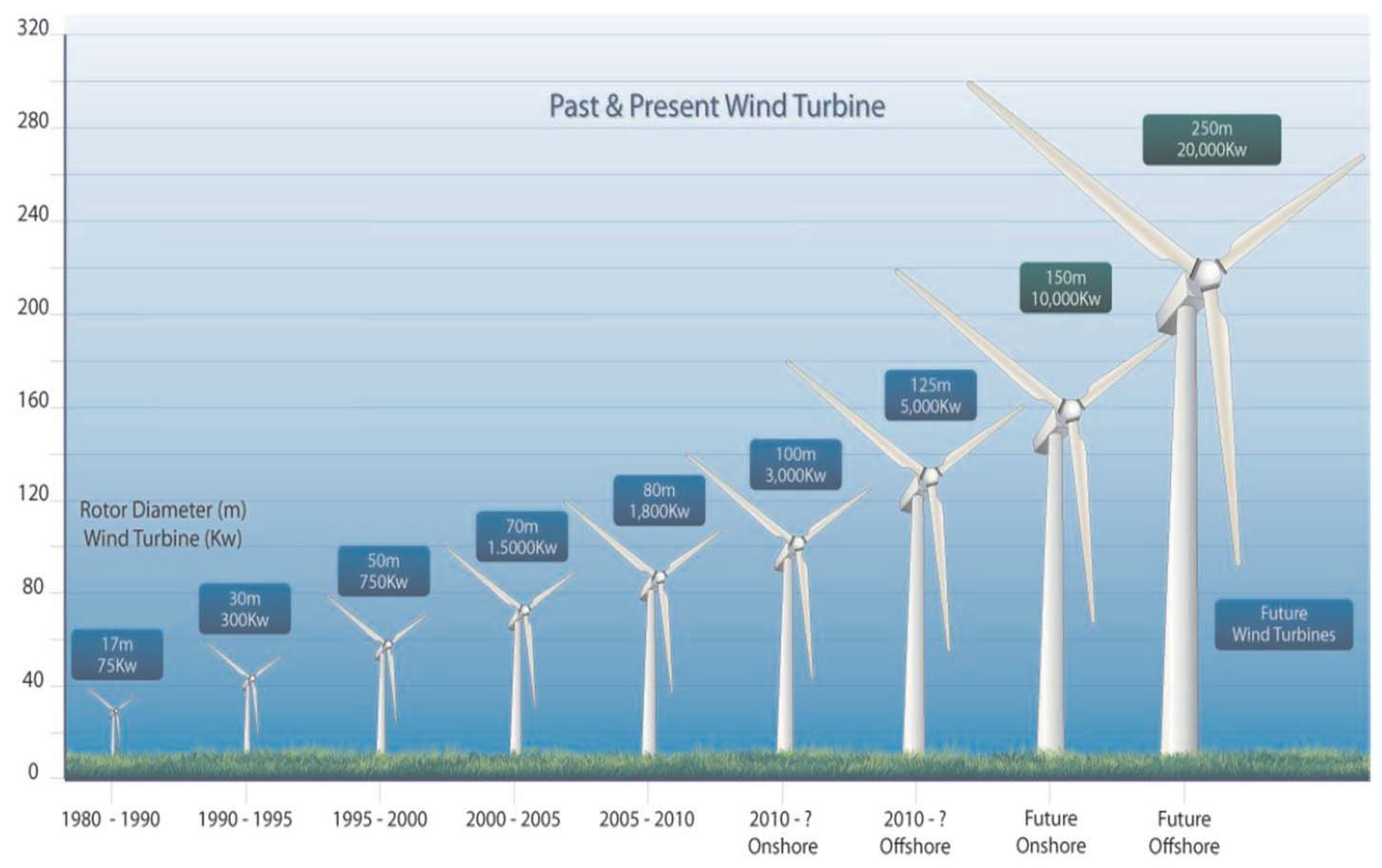
Figure 1 shows how the global wind power installations are 369.6 GW in 2014, with an expected growth to 415.7 GW by the end of 2015. After 2009, more than $50\%$ of new wind power resources were increased outside of the original markets of Europe and U.S., mainly motivated by the market growth in China, which now has 101,424 MW of wind power installed [2]. Several other countries have obtained quite high levels of stationary wind power production, with rates from $9\%$ to $21\%$, such as in Denmark, Portugal, Spain, France, Ireland, Germany, Ireland, Sweden in 2015 [2]. From 2009, 83 countries around the world are exploiting wind energy on a commercial basis, as wind power is considered as a renewable, sustainable and green solution for energy harvesting. Note however that, even if the U.S. now achieves less than $2\%$ of its required electrical energy from wind, the most recent NREL’s report states that the U.S. will increase it up to $30\%$ by the year 2030 [2]. Note also that, even if the fast growth of the wind turbine installed capacity of wind turbines in recent years, multidisciplinary engineering and science challenges still exist [3]. Moreover, wind turbine installations must guarantee both power capture and economical advantages, thus motivating the wind turbine dramatic growth as represented in Figure 2 [2].

Figure 2. Size growth of commercial wind turbines (hub heigh in m.).

Figure 2. Size growth of commercial wind turbines (hub heigh in m.).

Industrial wind turbines have large rotors and flexible load-carrying structures that operate in uncertain and noisy environments, thus motivating challenging cases for advanced control solutions [4]. Advanced controllers can be able to achieve the required goal of decreasing the wind energy cost by increasing the capture efficacy; at the same time they should reduce the structural loads, thus increasing the lifetimes of the components and turbine structures [4,5].

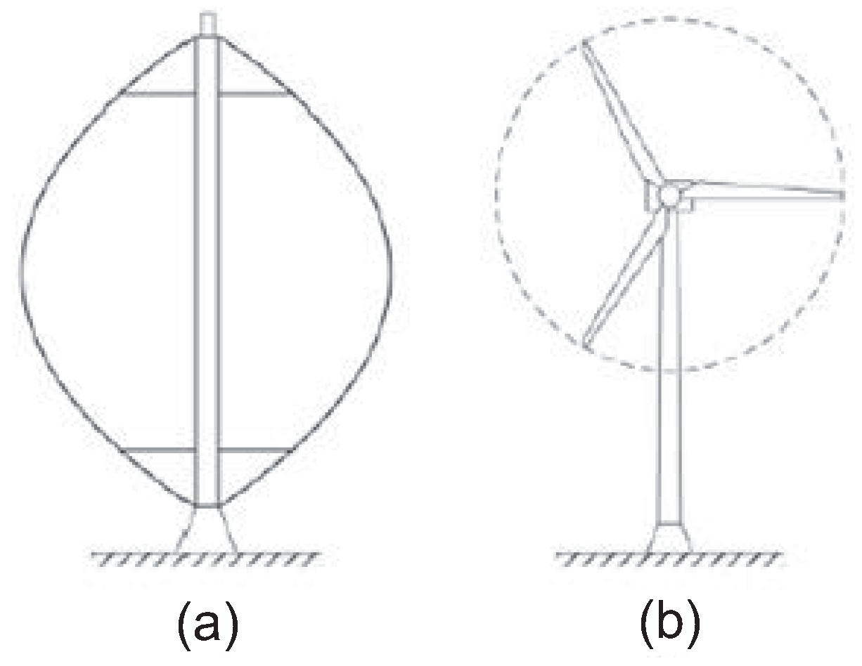
This review paper aims also at sketching the main challenges and the most recent research topics in this area. Although wind turbines can be developed in both vertical-axis and horizontal-axis configurations, as shown in Figure 3, this paper is focussed on horizontal-axis wind turbines, which represent the most common solutions today in produced large-scale installations.

Figure 3. Example of (a) vertical-axis; and (b) horizontal-axis wind turbines.

Figure 3. Example of (a) vertical-axis; and (b) horizontal-axis wind turbines.

Horizontal-axis wind turbines have the advantage that the rotor is placed atop a tall tower, with the advantage of larger wind speeds that the ground. Moreover, they can include pitchable blades in order to improve the power capture, the structural performance, and the overall system stability [6,7]. On the other hand, vertical-axis wind turbines are more common for smaller installations. Note finally that proper wind turbine models are usually oriented to the design of suitable control strategies that are more effective for large rotor wind turbines. Therefore, the most recent research focus considers wind turbines with capacities of more than 10 MW.

Another important issue derives from the increasing complexity of wind turbines, which gives rise to more strict requirements in terms of safety, reliability and availability [4]. In fact, due to the increased system complexity and redundancy, large wind turbines are prone to unexpected malfunctions or alterations of the nominal working conditions. Many of these anomalies, even if not critical, often lead to turbine shutdowns, again for safety reasons. Especially in offshore wind turbines, this may result in a substantially reduced availability, because rough weather conditions may prevent the prompt replacement of the damaged system parts. The need for reliability and availability that guarantees the continuous energy production requires the so-called “sustainable” control solutions [4,8]. These schemes should be able to keep the turbine in operation in the presence of anomalous situations, perhaps with reduced performance, while managing the maintenance operations. Apart from increasing availability and reducing turbine downtimes, sustainable control schemes might also obviate the need for more hardware redundancy, if virtual sensors could replace redundant hardware sensors [9]. These schemes currently employed in wind turbines are typically on the level of the supervisory control, where commonly used strategies include sensor comparison, model comparison and thresholding tests [1,9,10]. These strategies enable safe turbine operations, which involve shutdowns in case of critical situations, but they are not able to actively counteract anomalous working conditions. Therefore, the goal of this work is also to investigate these so-called sustainable control strategies, which allow to obtain a system behaviour that is close to the nominal situation in presence of unpermitted deviations of any characteristic properties or system parameters from standard conditions (i.e., a fault) [8,11]. Moreover, these schemes should provide the reconstruction of the equivalent unknown input that represents the effect of a fault, thus achieving the so-called fault diagnosis task [9,10].

It is worth noting that the present paper and e.g., the work [12] share some common issues. However, this paper is also presenting some advanced aspects regarding advanced modelling topics [13], as well as the very recent and advanced task concerning the sustainable control for wind turbines [14,15], which is fundamental for large rotors and offshore installations.

The rest of this paper is organised as follows. Section 2 describes the basic configurations and operations of wind turbines. Section 3 explains the layout of the wind turbine main control loops, including the wind characteristics, the available sensors and actuators commonly used in advanced control. Section 4 describes the basic structure of the typical wind turbine control, which is then followed by a brief discussion of advanced control opportunities in Section 5. On the other hand, Section 5.1 outlines the main sustainable control strategies recently proposed for wind turbines. Concluding remarks are finally summarised in Section 6.

2. Wind Turbine Modelling Issues

Prior to apply any new control strategies on a real wind turbine, the efficacy of the control scheme has to be tested in detailed aero-elastic simulation model. Several simulation packages exist that are commonly used in academia and industry for wind turbine load simulation. This paper recalls one of the most used simulation package, that is the Fatigue, Aerodynamics, Structures, and Turbulence (FAST) code [16] provided by NREL, since it represents a reference simulation environment for the development of high-fidelity wind turbine prototypes that are taken as a reference test-cases for many practical studies [4,17].

FAST provides a high-fidelity wind turbine model with 24 degrees of freedom, which is appropriate for testing the developed control algorithms but not for control design. For the latter purpose, a reduced-order dynamic wind turbine model, which captures only dynamic effects directly influenced by the control, is recalled in this section and it can be used for model-based control design. It almost corresponds to the model presented in [4].

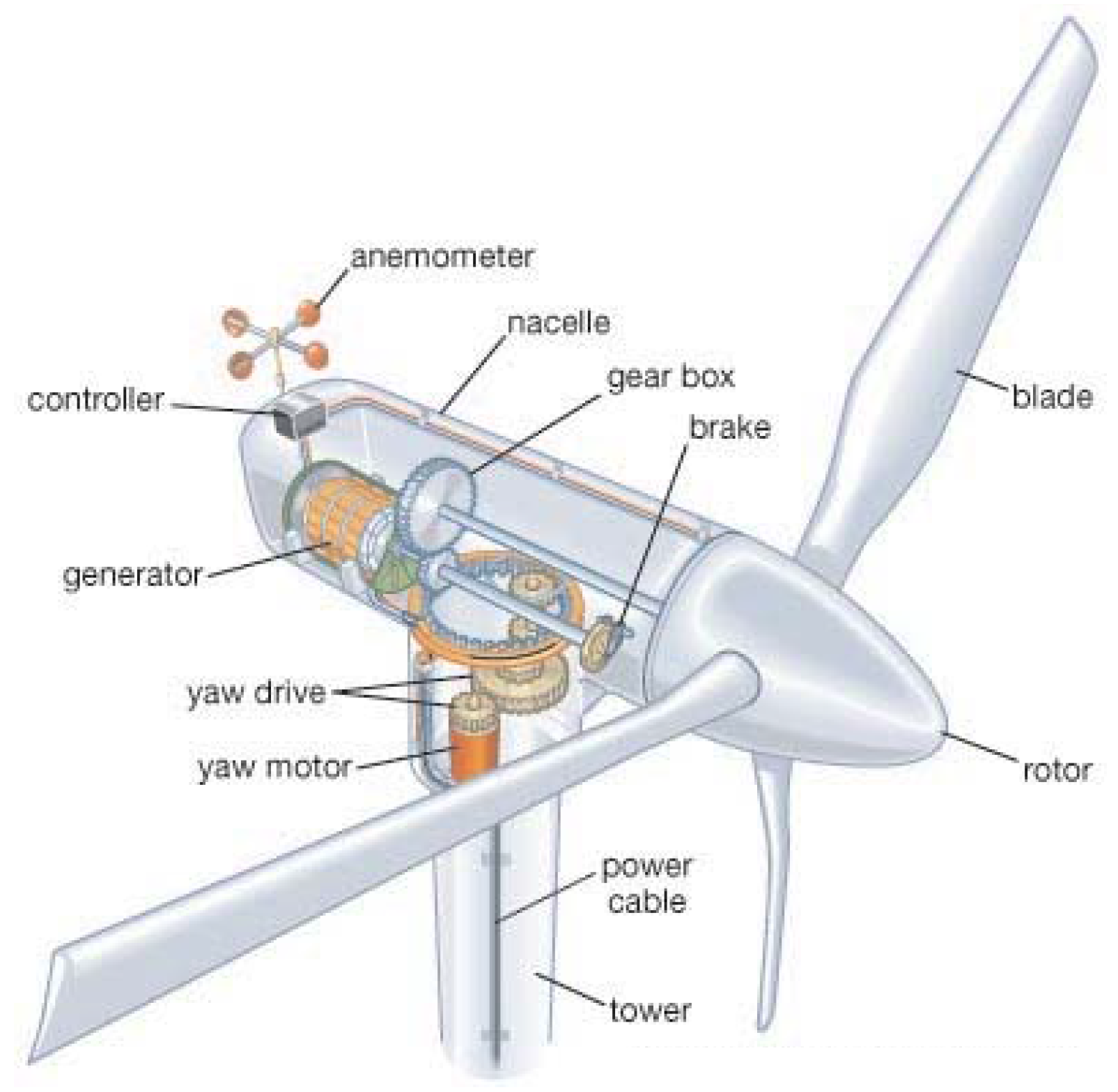
The main components of a horizontal-axis wind turbine are its tower, nacelle, and rotor, as shown in Figure 4. The generator is placed in the nacelle, and it is driven by the high-speed shaft, connected by a gear box to the low-speed shaft of the rotor. The rotor includes the airfoil-shaped blades that are used to capture the wind energy.

Figure 4. Main wind turbine components.

Figure 4. Main wind turbine components.

Figure 5 sketches the complete wind turbine model consisting of several submodels for the mechanical structure, the aerodynamics, as well as the dynamics of the pitch system and the generator/converter system. The generator/converter dynamics are usually described as a first order delay system, as described e.g., in [4], as it represents a realistic assumption for control-oriented modelling. However, when the delay time constant is very small, an ideal converter can be assumed, such that the reference generator torque signal is equal to the actual generator torque. In this situation, the generator torque can be considered as a system input [4].

Figure 5. Block diagram of the complete wind turbine model.

Figure 5. Block diagram of the complete wind turbine model.

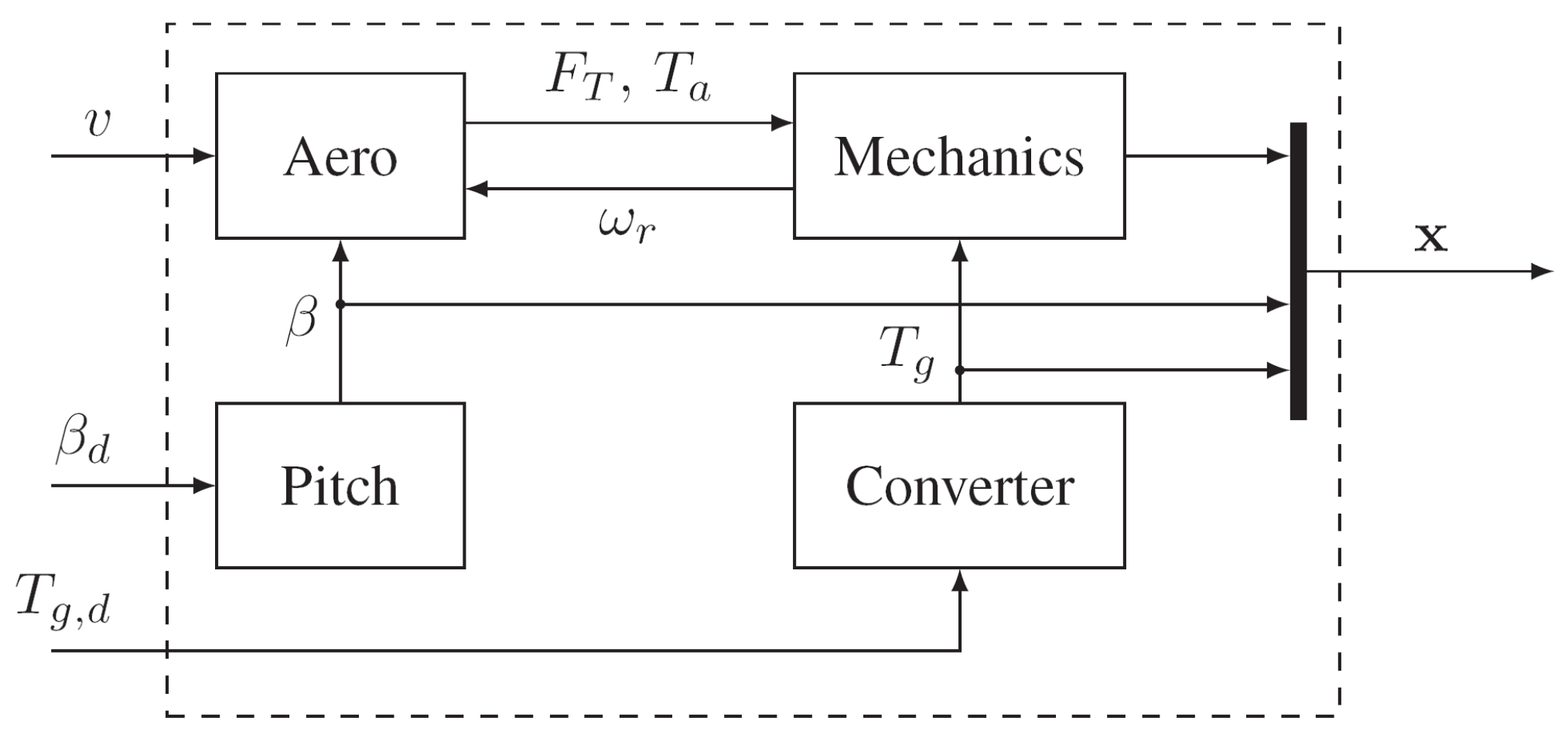
Figure 5 reports also the wind turbine inputs and outputs. In particular, v is wind speed; $F_T$ and $T_a$ correspond to the rotor thrust force and rotor torque, respectively; ${\omega }_r$ is the rotor angular velocity; x the state vector; $T_g$ the generator torque; and $T_{g,d}$ the demanded generator torque. β is the pitch angle, whilst ${\beta }_d$ its demanded value.

2.1. Wind Turbine Tower and Blade Models

As an example, a mechanical wind turbine model with four degrees of freedom is considered, since these degrees of freedom are the most strongly affected by the wind turbine control. In particular, they represent the fore-aft tower bending, the flap-wise blade bending, the rotor rotation, and the generator rotation [18].

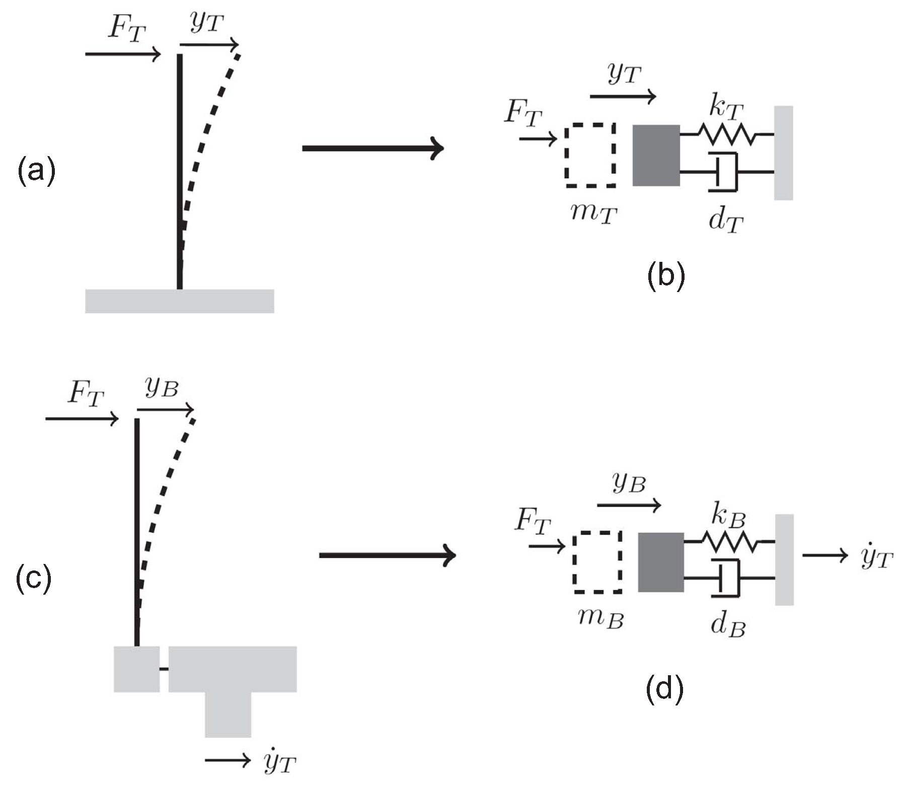
Both the tower and blade bending are not modelled by means of bending beam models, but only the translational displacement of the tower top and the blade tip are considered, where the bending stiffness parameters are transformed into equivalent translational stiffness parameters, as depicted in Figure 6.

Figure 6. (a) Tower bending; (b) Mechanical model with spring and damper; (c) Blade bending; and (d) Mechanical model [19].

Figure 6. (a) Tower bending; (b) Mechanical model with spring and damper; (c) Blade bending; and (d) Mechanical model [19].

With reference to Figure 6, the force $F_T$ generates the tower displacement $y_T$, which is modelled by the mechanical model of mass $m_T$, with spring and damper parameters $k_T$ and $d_T$, respectively. For the tower, the equivalent translational stiffness parameter is derived by means of a direct stiffness method common in structural mechanics calculations [18,19]. In the same way, the blade displacement $y_B$ generated by the force $F_T$ is described again as a mass $m_B$ with a spring and damper model, whose parameters are $k_B$ and $d_B$, respectively.

Since the blades move with the tower, the blade tip displacement $y_B$ is considered in the moving tower coordinate system and the tower motion must be taken into account for the derivation of the kinetic energy of the blade. The force $F_T$ acts both on the tower and on N blades. Only one collective blade degree of freedom is considered. Note that the N blade degrees of freedom would have to be considered individually if control strategies for load reduction involving individual blade pitch control were designed. The assumption that the same external force $F_T$ acts on both the tower and the blade degrees of freedom (with N blades) is a simplification. It is reasonable, however, because the rotor thrust force, which is caused by the aerodynamic lift forces acting on the blade elements, acts on the tower top, thus causing a distributed load on each blade. This distributed load generates a bending of the blade, which could be modelled as a bending beam. A beam subjected not to a distributed load but to a concentrated load at the upper point must have a higher bending beam stiffness, in order that the same displacement results at the upper point. However, a reduced-order wind turbine model considers only the blade tip displacement, which requires the assumption of a translational stiffness. To obtain an adequate translational stiffness constant, the bending stiffness of the bending beam must thus be larger than the case of a distributed load.

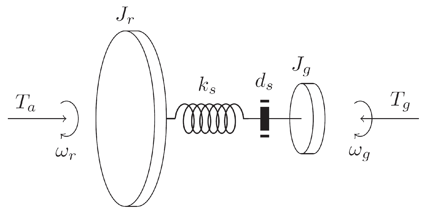
On the other hand, the drivetrain consisting of rotor, shaft and generator is modelled as a two-mass inertia system, including shaft torsion, where the two inertias are connected with a torsional spring with spring constant $k_S$ and a torsional damper with damping constant $d_S$, as illustrated in Figure 7 [19].

Figure 7. Drivetrain model.

Figure 7. Drivetrain model.

With reference to Figure 7, the angular velocities ${\omega }_r$ and ${\omega }_g$ are the time derivatives of the rotation angles ${\theta }_r$ and ${\theta }_g$. In this case, the rotor torque $T_a$ is generated by the lift forces on the individual blade elements, whilst $T_g$ represents the generator torque. The ideal gearbox effect can be simply included in the generator model by multiplying the generator inertia $J_g$ by the square of the gearbox ratio $n_g$.

The motion equations are derived by means of Lagrangian dynamics, which first requires one to define the generalised coordinates and generalised external forces. In this way, the energy terms of the system are derived, as well as the motion equations. The vector of generalised coordinates is given by: $\mathbf{q}={\left[y_T,y_B,{\theta }_r,{\theta }_g\right]}^T$, whilst the vector of external forces is defined as $\mathbf{f}=\left[F_T,F_T,T_a,-T_g\right]$.

The generalised force $F_T$ represents the rotor thrust force, which can be computed from the wind speed at the blade and from the aerodynamic map of the thrust coefficient. On the other hand, the generalised torque $T_a$ is given by the aerodynamic rotor torque, which can be calculated from the wind speed and from the aerodynamic map of the torque coefficient described in Section 2.4. By considering the tower dynamics, the complete blade tip displacement is given by $y_T+y_B$, and the kinetic energy has the following form:

$$E_K=\frac{1}{2}{m}_T{\dot{y}}_T^2+\frac{1}{2}N{m}_B{\left({\dot{y}}_T+{\dot{y}}_B\right)}^2+\frac{1}{2}{J}_r{\dot{\theta }}_r^2+\frac{1}{2}{J}_g{\dot{\theta }}_g^2$$

(1)

In the same way, the potential energy has the form:

$$E_P=\frac{1}{2}{k}_T{y}_T^2+\frac{1}{2}N{k}_B{y}_B^2+\frac{1}{2}{k}_S{\left({\theta }_r-\frac{1}{n_g}{\theta }_g\right)}^2$$

(2)

with $n_g$ the gearbox ratio. The dampings in the system produce generalised friction forces, which can be written as derivatives of a quadratic form, e.g., the dissipation function [20]. In this case, it assumes the form:

$$P_D=\frac{1}{2}{d}_T{\dot{y}}_T^2+\frac{1}{2}N{d}_B{\dot{y}}_B^2+\frac{1}{2}{d}_S{\left({\dot{\theta }}_r-\frac{1}{n_g}{\dot{\theta }}_g\right)}^2$$

(3)

The Lagrangian equations of second order including the dissipation term are given by [20]:

$$\frac{d}{dt}\left(\frac{\partial L}{\partial {\dot{q}}_i}\right)-\frac{\partial L}{\partial q_i}=f_i-\frac{\partial P_D}{\partial {\dot{q}}_i}$$

(4)

where the Lagrangian function L denotes the difference between kinetic and potential energy. As the kinetic energy in Equation (1) does not depend on the generalised coordinates and the potential energy in Equation (2) does not depend on the generalised velocities, the motion equations in the following form are obtained:

$$\left\{\begin{array}{ccc}\hfill \left(m_T+N{m}_B\right){\ddot{y}}_T+N{m}_B{\ddot{y}}_B+d_T{\dot{y}}_T+k_T{y}_T& =& F_T\hfill \\ \hfill N{m}_B{\ddot{y}}_T+N{m}_B{\ddot{y}}_B+NdB{\dot{y}}_B+N{k}_B{y}_B& =& F_T\hfill \\ \hfill J_r{\ddot{\theta }}_r+d_S\left({\omega }_r-\frac{1}{n_g}{\omega }_g\right)+k_S\left({\theta }_r-\frac{1}{n_g}{\theta }_g\right)& =& T_a\hfill \\ \hfill J_r\frac{1}{n_g}{\ddot{\theta }}_g-d_S\left({\omega }_r-\frac{1}{n_g}{\omega }_g\right)-k_S\left({\theta }_r-\frac{1}{n_g}{\theta }_g\right)& =& -T_g\hfill \end{array}\right.$$

(5)

The system Equation (5) can be rewritten in matrix form as:

$$\mathbf{M}\ddot{q}+\mathbf{D}\dot{q}+\mathbf{K}q=\mathbf{f}$$

(6)

where the mass matrix $\mathbf{M}$; the damping matrix $\mathbf{D}$ and the stiffness matrix $\mathbf{K}$ have the form:

$$\begin{array}{cc}\mathbf{M}=\left[\begin{array}{cccc}{m}_T+N{m}_B& N{m}_B& 0& 0\\ N{m}_B& N{m}_B& 0& 0\\ 0& 0& J_r& 0\\ 0& 0& 0& J_g\end{array}\right],\hfill & \mathbf{D}=\left[\begin{array}{cccc}{d}_T& 0& 0& 0\\ 0& N{d}_B& 0& 0\\ 0& 0& d_S& -\frac{d_S}{n_g}\\ 0& 0& -\frac{d_S}{n_g}& \frac{d_S}{n_g^2}\end{array}\right],\hfill \\ \mathbf{K}=\left[\begin{array}{cccc}{k}_T& 0& 0& 0\\ 0& N{k}_B& 0& 0\\ 0& 0& k_S& -\frac{k_S}{n_g}\\ 0& 0& -\frac{k_S}{n_g}& \frac{k_S}{n_g^2}\end{array}\right]\hfill \end{array}$$

(7)

The second order system of differential equations Equation (6) can be transformed into a first order state-space model by introducing the state vector $x={\left[q,\dot{q}\right]}^T$. To this aim, the expression Equation (6) is solved with respect to the second time derivative of the coordinate vector $\mathbf{q}$. The equivalent state-space model is thus obtained in the form:

$$\left\{\begin{array}{ccc}\dot{\mathbf{x}}\hfill & =& {\mathbf{A}}_m\mathbf{x}+{\mathbf{B}}_m{\mathbf{u}}_m\hfill \\ \mathbf{y}\hfill & =& {\mathbf{C}}_m\mathbf{x}\hfill \end{array}\right.$$

(8)

where the state vector is given by $\mathbf{x}={\left[y_T,y_B,{\theta }_r,{\theta }_g,{\dot{y}}_T,{\dot{y}}_B,{\dot{\theta }}_r,{\dot{\theta }}_g\right]}^T$; the input vector is ${\mathbf{u}}_m={\left[F_T,T_a,T_g\right]}^T$, whilst the system matrices have the form:

$$\begin{array}{cccc}{\mathbf{A}}_m=\left[\begin{array}{cc}{0}_{4\times 4}& I_{4\times 4}\\ -{\mathbf{M}}^{-1}\mathbf{K}& -{\mathbf{M}}^{-1}\mathbf{D}\end{array}\right],\hfill & {\mathbf{B}}_m=\left[\begin{array}{c}{0}_{4\times 3}\\ {\mathbf{M}}^{-1}\mathbf{Q}\end{array}\right],\hfill & {\mathbf{C}}_m={\mathbf{I}}_{8\times 8},\hfill & \mathrm{with}\mathbf{Q}=\left[\begin{array}{ccc}1& 0& 0\\ 1& 0& 0\\ 0& 1& 0\\ 0& 0& -1\end{array}\right]\hfill \end{array}$$

(9)

2.2. Pitch Model

In pitch-regulated wind turbines, the pitch angle of the blades is controlled only when working above the rated wind speed (“full-load” condition, as described in the following) to reduce the aerodynamic rotor torque, thus maintaining the turbine at the desired rotor speed. Moreover, the pitching of the blades to feather position (i.e., ${90}^o$) is used as main braking system to bring the turbine to standstill in critical situations. Two different pitch technologies are usually implemented using hydraulic and electromechanical actuation systems. For hydraulic pitch systems, the dynamics are described with a second-order model [4], which is able to include oscillatory behaviour. On the other hand, electromechanical pitch systems are usually described as a first-order model, which is represented by Equation (10):

$$\dot{\beta }=-\frac{1}{\tau }\beta +\frac{1}{\tau }{\beta }_d$$

(10)

where β and ${\beta }_d$ are the physical and the demanded pitch angle, respectively; The parameter τ denotes the delay time constant.

2.3. Generator/Converter Dynamic Model

A description of the generator/converter dynamics can be included into the complete wind turbine system model. Note that simulation-oriented models do not include it, since the generator/converter dynamics are relatively fast. However, when advanced control designs have to be investigated, an explicit generator/converter model might be required. In this situation, a simple first order delay model can be sufficient, as described e.g., in [4]:

$${\dot{T}}_g=-\frac{1}{{\tau }_g}{T}_g+\frac{1}{{\tau }_g}{T}_{g,d}$$

(11)

where $T_{g,d}$ represents the demanded generator torque; whilst ${\tau }_g$ the delay time constant.

2.4. Aerodynamic Model

The aerodynamic submodel consists of the expressions for the thrust force $F_T$ acting on the rotor and the aerodynamic rotor torque $T_a$. They are determined by the reference force $F_{st}$ and by the aerodynamic rotor thrust and torque coefficients $C_T$ and $C_Q$ [18]:

$$\left\{\begin{array}{ccc}{F}_T\hfill & =& F_{st}{C}_T\left(\lambda ,\beta \right)\hfill \\ T_a\hfill & =& F_{st}R{C}_Q\left(\lambda ,\beta \right)\hfill \end{array}\right.$$

(12)

The reference force $F_{st}$ is defined from the impact pressure $\frac{1}{2}\rho v^2$ and the rotor swept area $\pi R^2$ (with rotor radius R), where ρ denotes the air density:

$$F_{st}=\frac{1}{2}\rho \pi R^2{v}^2$$

(13)

It is worth noting that simulation-oriented benchmarks use the static wind speed v. However, more accurate scenarios should exploit the effective wind speed $v_e=v-\left({\dot{y}}_T+{\dot{y}}_B\right)$, i.e., the static wind speed corrected with by the tower and blade motion effects. However, the aerodynamic maps used for the calculation of the rotor thrust and torque are usually represented as static 2-dimensional tables, which already take into account the dynamic contributions of both the tower and the blade motions.

As highlighted in the expressions Equation (12), the rotor thrust and torque coefficients $\left(C_T,C_Q\right)$ depend on the tip speed ratio $\lambda =\frac{{\omega }_{r}R}{v}$ and the pitch angle β. Therefore, the rotor thrust $F_T$ and torque $T_a$ assume the following expressions:

$$\left\{\begin{array}{ccc}{F}_T\hfill & =& \frac{1}{2}\rho \pi R^2{C}_T\left(\lambda ,\beta \right)v^2\hfill \\ T_a\hfill & =& \frac{1}{2}\rho \pi R^3{C}_Q\left(\lambda ,\beta \right)v^2\hfill \end{array}\right.$$

(14)

The expressions Equation (14) highlight that the rotor thrust $F_T$ and torque $T_a$ are nonlinear functions that depend on the wind speed v, the rotor speed ${\omega }_r$, and the pitch angle β. These functions are usually expressed as two-dimensional maps, which must be known for the whole range of variation of both the pitch angles and tip speed ratios. These maps are usually a static approximation of more detailed aerodynamic computations that can be obtained using for example the Blade Element Momentum (BEM) method. In this case, the aerodynamic lift and drag forces at each blade section are calculated and integrated in order to obtain the rotor thrust and torque [18]. More accurate maps can be obtained by exploiting the calculations implemented via the AeroDyn module of the FAST code, where the maps are extracted from several simulation runs [21].

It is worth noting that for simulation purposes, the tabulated versions of the aerodynamic maps $C_Q$ and $C_T$ are sufficient. On the other hand, for control design, the derivatives of the rotor torque (and thrust) are needed, thus requiring a description of the aerodynamic maps as analytical functions. Therefore, these maps can be approximated using combinations of polynomial and exponential functions, whose powers and coefficients are estimated via e.g., modelling [22] or identification [23,24] approaches.

2.5. Wind Turbine Overall Model

By replacing the expressions Equation (14) for the rotor thrust and torque into the mechanical model Equation (8) and adding the models Equations (10) and (11) for the pitch and the generator/converter dynamics, a nonlinear state-space model is obtained:

$$\left\{\begin{array}{ccc}\dot{\mathbf{x}}\hfill & =& \mathbf{A}\mathbf{x}+\mathbf{B}\mathbf{u}+g\left(\mathbf{x},v\right)\hfill \\ \mathbf{y}\hfill & =& \mathbf{C}\mathbf{x}\hfill \end{array}\right.$$

(15)

with a state vector that now includes the pitch angle and the generator torque: $\mathbf{x}={\left[y_T,y_B,{\theta }_r,{\theta }_g,{\dot{y}}_T,{\dot{y}}_B,{\dot{\theta }}_r,{\dot{\theta }}_g,\beta \right]}^T$. Since the rotor thrust force and the rotor torque have been used as inputs for the vector ${\mathbf{u}}_m$ in the mechanical submodel Equation (8), a new input vector is defined for the complete state-space model Equation (15), i.e., $\mathbf{u}={\left[{\beta }_d,T_g\right]}^T$ , whose components are the demanded pitch angle and the generator torque, respectively. The wind speed is normally considered as a disturbance input. The linear part of the state-space model Equation (15) is defined by the matrices:

$$\begin{array}{cc}\mathbf{A}=\left[\begin{array}{cccc}{0}_{3\times 3}& \tilde{\mathbf{L}}& 0_{3\times 1}& 0_{3\times 1}\\ {\mathbf{M}}^{-1}\tilde{\mathbf{K}}& {\mathbf{M}}^{-1}\mathbf{D}& 0_{4\times 1}& \left[\begin{array}{c}{0}_{3\times 1}\\ -\frac{1}{J_g}\end{array}\right]\\ 0_{1\times 3}& 0_{1\times 4}& -\frac{1}{\tau }& 0\\ 0_{1\times 3}& 0_{1\times 4}& 0& -\frac{1}{{\tau }_g}\end{array}\right],\hfill & \mathbf{B}=\left[\begin{array}{cc}{0}_{7\times 1}& 0_{7\times 1}\\ \frac{1}{\tau }& 0\\ 0& -\frac{1}{{\tau }_g}\end{array}\right]\hfill \end{array}$$

(16)

with:

$$\begin{array}{cc}\tilde{\mathbf{L}}=\left[\begin{array}{cccc}1& 0& 0& 0\\ 0& 1& 0& 0\\ 0& 0& 1& -1\end{array}\right]\hfill & \mathrm{and}\tilde{\mathbf{K}}=\left[\begin{array}{ccc}{k}_T& 0& 0\\ 0& N{k}_B& 0\\ 0& 0& k_S\\ 0& 0& -k_S\end{array}\right]\hfill \end{array}$$

(17)

Moreover, the system vector in Equation (15) nonlinearly depends on the state and input vector:

$$g\left(\mathbf{x},v\right)=\left[\begin{array}{c}{0}_{4\times 1}\\ \frac{1}{m_B}{F}_T\left(\mathbf{x},v\right)\\ \frac{1}{J_r}{T}_a\left(\mathbf{x},v\right)\\ 0_{3\times 1}\end{array}\right]$$

(18)

Here, the rotor thrust and torque expressions are given in Equation (14), whilst the mass and damping matrices are defined in Equation (7).

It is worth noting that in a real wind turbine, the centrifugal forces acting on the rotating rotor blades lead to a stiffening of the blades. As a consequence, the bending behaviour of the rotor blades depends on the rotor speed itself. By considering again the translational spring-mass system of the blade-tip displacement, this second-order effect can be included in the model Equation (15) by introducing a translational blade stiffness parameter $k_B$ dependent on the rotor speed, i.e., $k_B\left({\omega }_r\right)=\alpha m_B{r}_B{\omega }_r^2$. $r_B$ denotes the distance from the blade root to the blade centre of mass and α tuning parameter. In this way, by including the centrifugal stiffening correction, the nonlinear system vector $g\left(\mathbf{x},v\right)$ in Equation (18) has the form:

$$g\left(\mathbf{x},v\right)=\left[\begin{array}{c}{0}_{3\times 1}\\ \frac{N}{m_T}{k}_B\left({\omega }_r\right)y_B\\ \frac{1}{N{m}_B}{F}_T\left(\mathbf{x},v\right)+\frac{m_T+N{m}_B}{m_T{m}_B}{k}_B\left({\omega }_r\right)y_B\\ \frac{1}{J_r}{T}_a\left(\mathbf{x},v\right)\\ 0_{3\times 1}\end{array}\right]$$

(19)

The inclusion of the centrifugal term is inspired from the FAST code, in order to obtain a high-fidelity wind turbine simulation model. For example, the translational blade bending model could be required when overspeed scenarios shall be taken into account. However, for the usual operating regimes of a wind turbine, the corrections induced by the centrifugal blade stiffening have only minor effects on the final results. Therefore, the centrifugal correction has been recalled here for the sake of completeness, but it has limited interest in real cases.

2.6. Measurement Errors

Wind turbine high-fidelity simulators, which were described e.g., in [4,25,26], consider white noise added to all measurements. This relies on the assumption that noisy sensor signals should represent more realistic scenarios. However, this is not the case, as a realistic simulation would require an accurate knowledge of each sensor and its measurement reliability. To the best of the author’s knowledge and from his experience with wind turbine systems for fault diagnosis and fault tolerant control [27,28], all main measurements acquired from the wind turbine process (rotor and generator speed, pitch angle, generator torque), are virtually noise-free or affected by very weak noise.

On the other hand, with reference to real wind turbines, one characteristic frequency is usually affecting the generator speed signal due to the periodic rotor excitation of the drivetrain. When using the generator speed as a controlled variable, a notch filter is thus applied to smooth the generator speed signal. Such a notch filter is usually applied to industrial wind turbine control as described e.g., in [29,30]. On the other hand, the rotor speed measurement is normally assumed to be a continuous signal. However, in many wind turbines, the rotor speed signal is discretised, due to the limited number of metal pieces on the main shaft that are scanned by a magnetic sensor, although better sensing technologies, which could yield nearly continuous signals, are already available, like optical scanning of densely spaced barcodes.

3. Basic Wind Turbine Control Issues

Wind turbine control methods depend on the turbine configuration. The horizontal-axis wind turbine can be “upwind”, if the rotor is on the upwind side of the tower, or “downwind”. This configuration affects the choice of the controller and the turbine dynamics, and thus the structural design. Wind turbines may also be variable pitch or fixed pitch, meaning that the blades may or may not be able to rotate along their longitudinal axes. The fixed-pitch strategy is less common in large wind turbines, due to the reduced ability to control loads and adapt the aerodynamic torque. On the other hand, variable-pitch turbines allow their blades to rotate along the pitch axis, thus modifying the aerodynamic characteristics. Moreover, wind turbines can be variable speed or fixed speed. Variable-speed turbines work closer to their maximum aerodynamic efficiency for a higher percentage of the time, but require electrical power converters and inverters for feeding the generated electricity into the grid at the proper frequency.

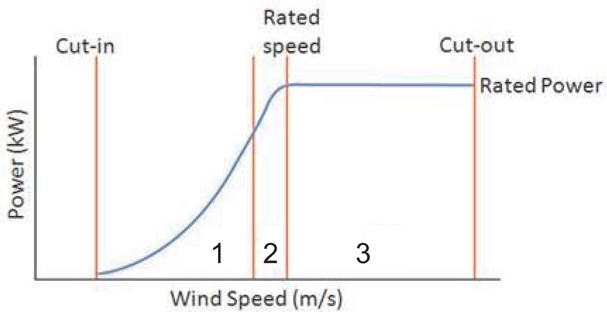
The effectiveness of the wind turbine power capture is described by Figure 8, which shows an example power curve for a variable-speed wind turbine of several kW of rated power. When the wind speed is low (usually below 6 m/s), the available wind power is lower that the turbine system losses, and the turbine is not working. This operational region is sometimes known as Region 1. When the wind speed is higher, i.e., the Region 3 (above $11.7$ m/s), power is limited to avoid exceeding safe electrical and mechanical load limits.

Figure 8. Example of wind turbine power curve.

Figure 8. Example of wind turbine power curve.

The main difference between fixed-speed and variable speed wind turbines appears for mid-range wind speeds, i.e., the Region 2 depicted in Figure 8, which includes wind speeds between 6 and $11.7$ m/s. Except for one design operating point (about 10 m/s), a variable-speed turbine captures more power than a fixed-speed turbine. The reason for the discrepancy is that variable-speed turbines can operate at maximum aerodynamic efficiency over a wider range of wind speeds than fixed-speed turbines. This difference can be up to about 150 kW in Region 2 [3]. Typical wind speed conditions allow a variable-speed turbine to capture about $2.3\%$ more energy per year than a constant-speed turbine, which represents a significant difference in the wind industry.

Figure 8 does not show the “high wind cut-out”, i.e., the wind speed above which the turbine is powered down and stopped to avoid excessive operating loads. High wind cut-out typically occurs at wind speeds higher that 20/30 m/s for large turbines.

Even an ideal wind turbine is not able to capture all the power available in the wind. This limitation is described by the actuator disc theory, which shows how the theoretical maximum aerodynamic efficiency, (called the Betz limit) is approximately $60\%$ of the wind power [31]. In fact, the wind must have some kinetic energy remaining after passing through the rotor disc. Otherwise, the wind would be stopped and no more wind would be able to pass through the rotor to provide energy to the turbine.

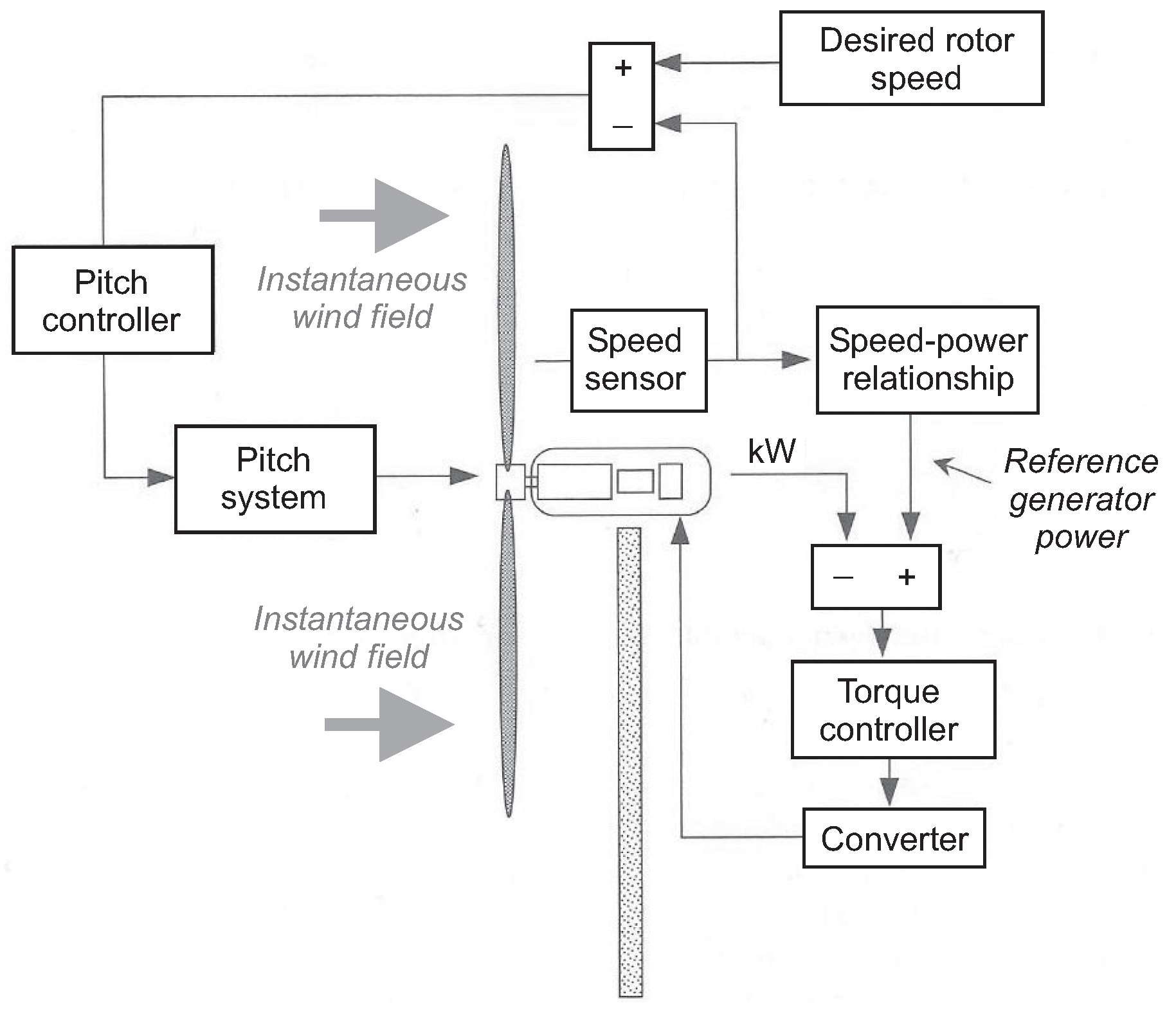
It is worth noting that the relation in Equation (14) assumes that the wind speed is uniform across the rotor plane. However, as indicated by the “instantaneous wind field” in Figure 9, the wind input can vary substantially in space and time as it approaches the rotor plane. The deviations of the wind speed from the expected nominal wind speed across the rotor plane are considered disturbances for control design. It is virtually impossible to obtain a good measurement of the wind speed encountering the blades because of the spatial and temporal variability and also because the rotor interacts with and changes the wind input. Not only does turbulent wind cause the wind to be different for the different blades, but the wind speed input is different at different positions along each blade. This issue represent an important aspect in the design of sustainable control solutions for large rotor wind turbines, as shown e.g., in [4,32,33].

Figure 9. Wind turbine basic control loops.

Figure 9. Wind turbine basic control loops.

Wind turbines can implement several levels of control, which are called “supervisory control”, “operational control”, and “subsystem control” [4,33].

The top-level supervisory control determines when the turbine starts and stops in response to changes in the wind speed, and also monitors the health of the turbine. The operational control determines how the turbine achieves its control objectives in the Regions 2 and 3. The subsystem controllers cause the generator, power electronics, yaw drive, pitch drive, and other actuators to perform as desired. The operational control loops and the controllers are shown in Figure 9, which exploit the submodels described in Section 2. In particular, the main control objectives, which are recalled in Section 3.1, will be exploited for illustrating the pitch and torque controllers in Section 4. These aspects represent key issues for the design of advanced and sustainable control solutions, as shown in Section 5 and Section 5.1.

3.1. Main Control Objectives

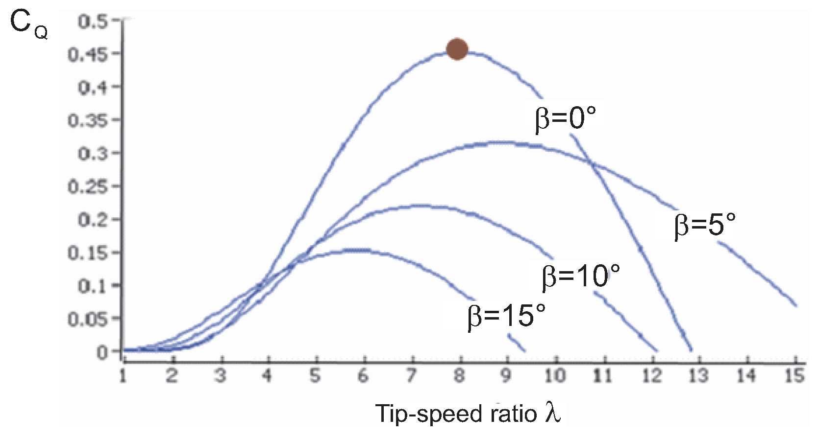
In the Region 2 a variable-speed wind turbine should maximise the power coefficient, and in particular the $C_Q$ map included in the expression Equation (12). Moreover, as remarked in Section 2.4, this power coefficient is a function of the turbine tip-speed ratio λ, defined as the ratio of the linear (tangential) speed of the blade tip and the wind speed. v and ${\omega }_r$ are always time-varying. The relationship between $C_Q$ and the tip-speed ratio λ is a nonlinear function depending on the particular turbine. As already remarked, $C_Q$ depends also on the blade pitch angle β in a nonlinear way, and these relationships have the same basic shape for most modern wind turbines. An example of $C_Q$ surface is shown in Figure 10 for a generic wind turbine.

Figure 10. Example of power coefficient curve.

Figure 10. Example of power coefficient curve.

Therefore, Figure 10 highlights that a turbine operates at its highest aerodynamic efficiency point, $C_{\max }$, given a certain pitch angle and tip-speed ratio. The pitch angle is quite easy to control, and can be suitably maintained at the optimal efficiency point. However, the tip-speed ratio depends on the wind speed v and therefore is always varying. Therefore, in the Region 2 the control objective at tracking the wind speed by varying the turbine speed. Section 4 will explain how this control objective can be achieved by using a simple scheme.

On the other hand, the control in Region 3 is typically achieved using a separate pitch control loop, as sketched in Figure 5 of Section 2. In the Region 3, the control objective has to limit the turbine power in order to maintain both the electrical and the mechanical loads at safe levels. This power limitation can be obtained also by yawing the turbine out of the wind, in order to reduce the aerodynamic torque. Note that the power P is related to rotor speed ${\omega }_r$ and aerodynamic torque $T_a$ by the simple relation:

$$P=T_a{\omega }_r$$

(20)

If the power and rotor speed are held constant, the aerodynamic torque must also be constant even if wind speed varies. The maximal power that can be safely produced by a wind turbine is defined as rated power. In this case, in the Region 3 the pitch controller modifies the rotor speed ${\omega }_r$ (at the turbine “rated speed”) so that the turbine operates at its rated power.

It is worth noting that the wind turbine blades may be controlled to all turn collectively or to each turn independently or individually. As outlined in Section 2.2, suitable pitch systems can be used to change the aerodynamic torque from the wind input, and are often fast enough to be of interest to the control community. Variable-pitch systems can limit their power either by pitching to “stall” or to “feather”. A discussion of the features of the collective or individual pitch control strategies is beyond the scope of this paper, but more information can be found e.g., in [6,18].

4. Basic Feedback Control Solutions for Wind Turbines

This section considers the basic control strategies that are typically used for the torque control and the pitch control blocks in Figure 5 of Section 2. As depicted in Figure 5, both control loops typically only use rotor speed feedback. The other sensors and measurements acquired from the wind turbine can be used for advanced control purposes, as outlined in Section 5.1.

It is worth noting that this paper considers the baseline control schemes that have been already considered e.g., in [4], as they represented the starting point for the development of sustainable control methodologies, as summarised e.g., in [15,34,35]. On the other hand, other advanced control strategies are recalled in Section 5.

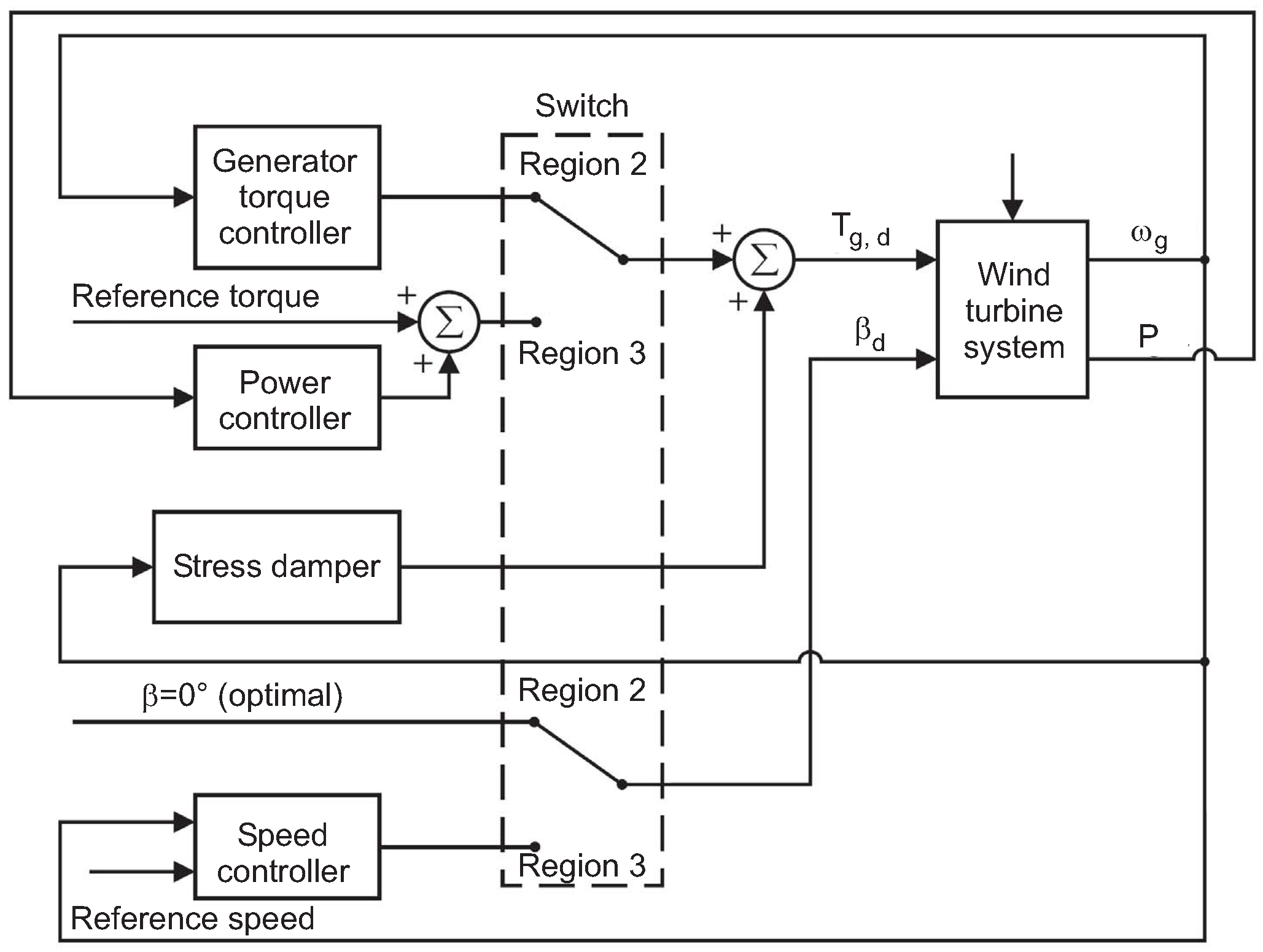
Therefore, by considering the baseline controllers addressed in [4], Figure 8 shows that the nominal operating condition is maintained to satisfy different demands below and above a certain wind speed. In this case, by following the classical control approach, the control task is divided into the design of multiple separate compensators, as highlighted in Figure 11.

Figure 11. Switching control structure.

Figure 11. Switching control structure.

Therefore, according to Figure 11, a switch reconfigures the control system to the current operating objectives between the Regions 2 and 3.

The design of the complete wind turbine controller can be devised into four basic control design steps, as listed below:

• Controller operating in partial load condition: it refers to the design of the generator torque controller. This controller operates in the partial load (Region 2), and should maximise the energy production while minimising mechanical stress and actuator usage;
• Controller operating in full load condition: it concerns the speed controller and power controller. These controllers operate in the full load (Region 3), and should track the rated generator speed and limiting the output power;
• Bumpless transfer: it describe the design of the mechanism that eliminates bumps on the control signals, when switching between the controllers in the partial load and full load regions;
• Structural stress damper: it regards the design of structure and drivetrain stress damper. The purpose of the module is to dampen drivetrain oscillations and reduce structural stress that could affect the wind turbine tower.

The first two items represent the main control loops, whilst the two other tasks concern some advanced control issues, which can enhance both the control and system performances.

In this way, the strategy of the complete controller of Figure 11 is to use two different controllers for the partial and the full load region. When the wind speed is below the rated value, the control system should maintain the pitch angle at its optimal value and control the generator torque in order to achieve the optimal tip-speed ratio (switch to the Region 2).

Above the rated wind speed the output power is kept constant by pitching the rotor blades, while using a power controller that manipulates the generator torque around a constant value to remove steady-state errors on the output power. This behaviour is obtained by setting the two switches in Figure 11 to the Region 3. In both regions a drivetrain stress damper is exploited to dampen drivetrain oscillations actively. Together, the two sets of controllers are able to solve the control task of tracking the ideal power curve in Figure 10. In order to switch smoothly between the two sets of controllers a bumpless transfer mechanism is implemented.

It is worth noting that in order to manage the transition between the Region 2 and the Region 3, an additional control region called Region 2.5 is considered [12]. The primary goal of the Region 2.5 control strategy is to connect Regions 2 and 3 controllers linearly. Unfortunately, this linear connection does not result in smooth transitions, and the discontinuous slopes in the torque control curve can contribute to excessive loading on the turbine. Therefore, this issue motivates the bumpless transfer recalled in Section 4.4. On the other hand, different nonlinear controllers were proposed by the same author e.g., in [34].

4.1. Partial Load Controller

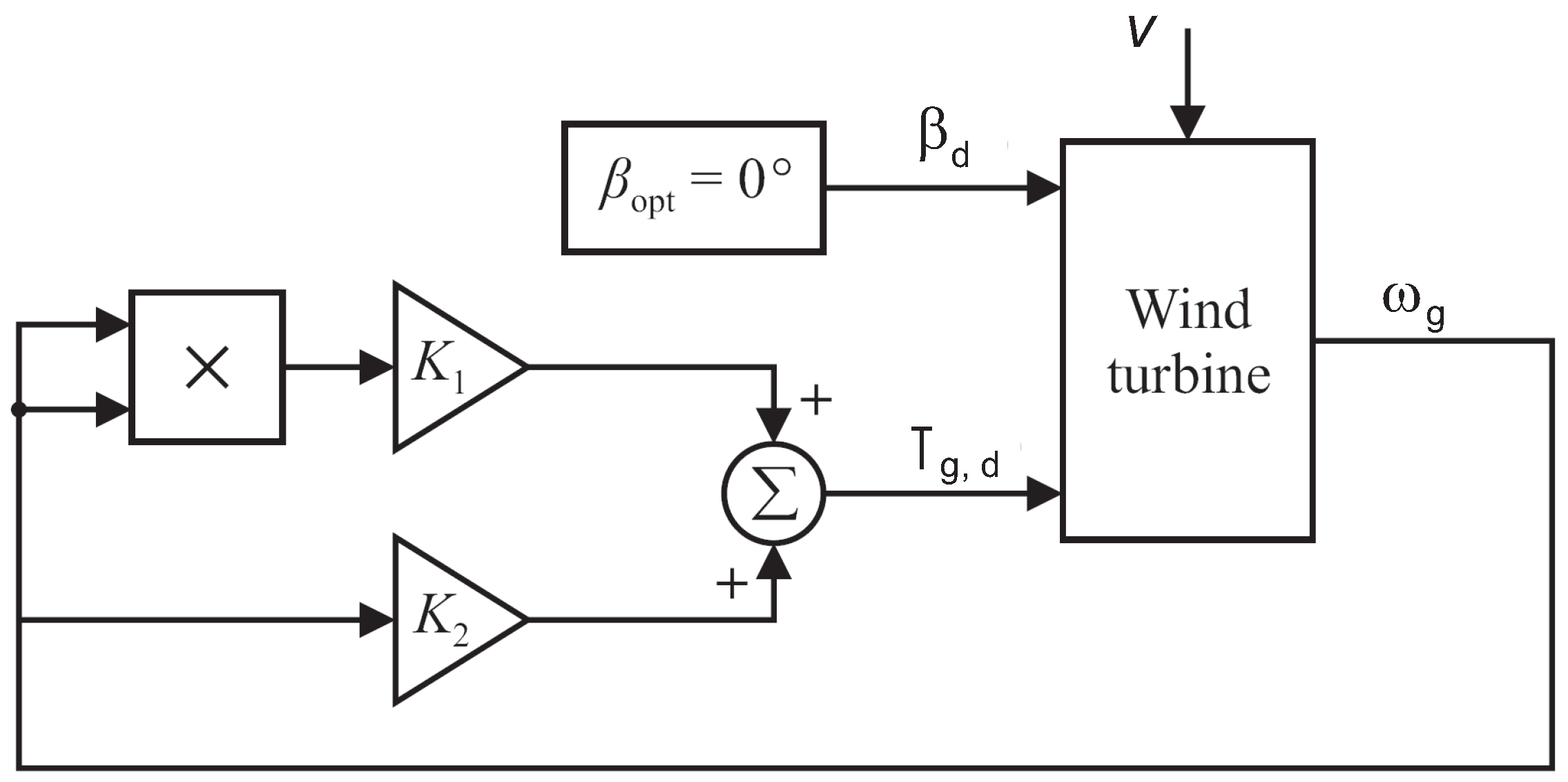
At low wind speeds, i.e., in partial load operation, variable-speed control is implemented to track the optimal point on the $C_Q$-surface for maximising the generated power. The speed of the generator is controlled by regulating the torque on the generator itself through the generator torque controller. Partial load operation leads to operate the wind turbine at $\beta =0^o$ since the maximum power coefficient is obtained at this pitch angle. This means that the highest efficiency is achieved for:

$${\lambda }_{\mathrm{opt}}=\frac{{\omega }_{r,\mathrm{opt}}R}{v}$$

(21)

where ${\lambda }_{\mathrm{opt}}$ is the tip-speed ratio maximising the $C_Q$-value for $\beta =0^o$; and ${\omega }_{r,\mathrm{opt}}$ is the optimum rotor speed. In order to obtain the optimal tip-speed ratio a method is used, which suggests to apply a certain generator torque as a function of the generator speed [36]. The advantage of this approach is that only the measurement of the rotor speed or generator speed is required. When utilising this approach, the controller structure for partial load operation is illustrated in Figure 12.

Figure 12. Generator torque controller for operation in partial load region (Region 2).

Figure 12. Generator torque controller for operation in partial load region (Region 2).

The principle of the standard control law is to calculate the wind speed in the definition of the tip-speed ratio, and replace it into the expression for the aerodynamic torque in Equation (14). Hence, the relation can be obtained expressing the required generator torque based on the maximum power coefficient and the optimal tip-speed ratio:

$$v\left(t\right)=\frac{{\omega }_r\left(t\right)R}{\lambda \left(t\right)}$$

(22)

This expression is inserted into Equation (14) describing the aerodynamic torque:

$$T_a\left(t\right)=\frac{1}{2}\rho \pi R^2\frac{R^3}{{\lambda }^3\left(t\right)}{C}_Q\left(\lambda \left(t\right),\beta \left(t\right)\right){\omega }_r^2\left(t\right)$$

(23)

Since the wind turbine includes a transmission system, the gear ratio and friction components of the drivetrain have to be considered when determining the generator torque corresponding to a certain aerodynamic torque. In order to describe the generator torque only as function of the generator speed, the system has to be assumed in steady-state, where ${\dot{\omega }}_r\left(t\right)={\dot{\omega }}_g\left(t\right)=0$ and ${\omega }_g\left(t\right)=n_g{\omega }_r\left(t\right)$. In this way, by considering the drivetrain equations in Equation (5), the following expression is obtained:

$$T_{g,d}=\frac{1}{2}\rho \pi R^2\frac{R^3}{n_g^3{\lambda }_{\mathrm{opt}}^3}{C}_{\max }{\omega }_g^2\left(t\right)-d_S\left(\frac{1}{n_g^2}+1\right){\omega }_g$$

(24)

with:

$$\begin{array}{cc}{K}_1=\frac{1}{2}\rho \pi R^2\frac{R^3}{n_g^3{\lambda }_{\mathrm{opt}}^3},\hfill & K_2=-d_S\left(\frac{1}{n_g^2}+1\right)\hfill \end{array}$$

(25)

It is worth noting that the term depending on ${\omega }_g$ represents the compensation of the frictions in the drivetrain, whose effects are not usually included in traditional control designs, proposed e.g., in [12,36], and thus motivating the need of advanced modelling aspects addressed in this paper.

4.2. Full Load Operation Controller

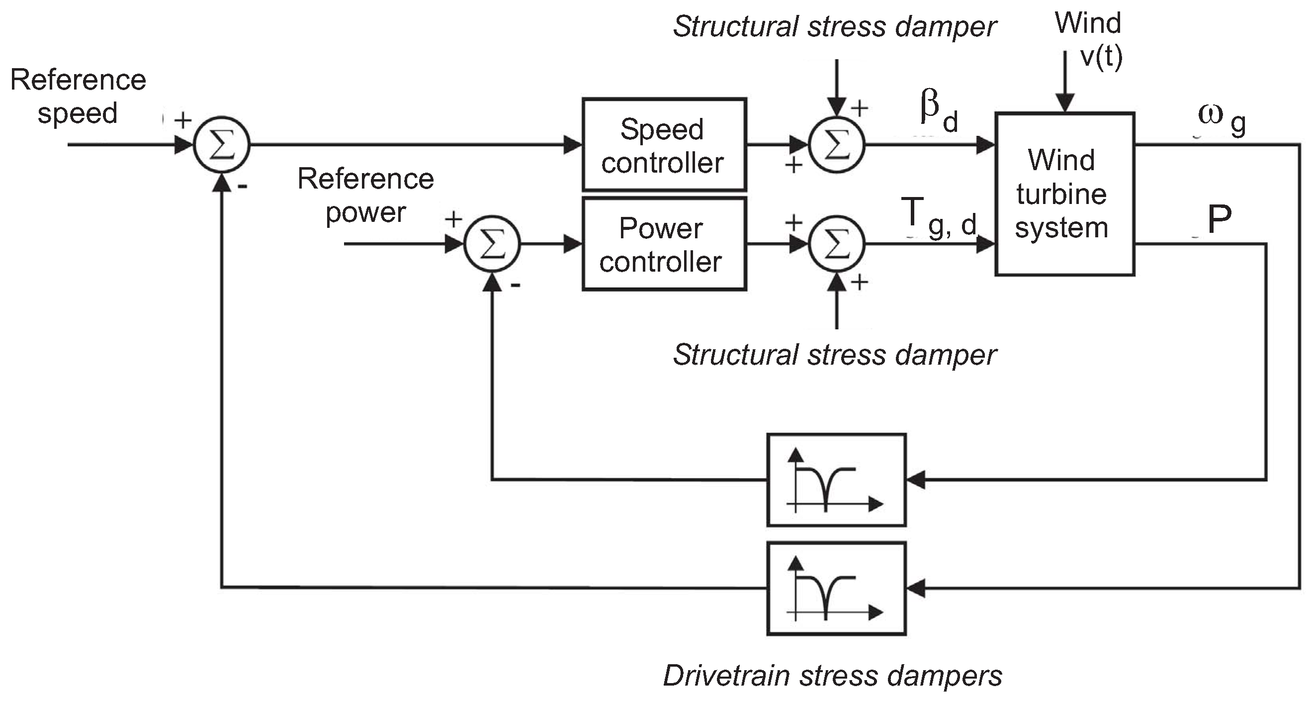
In full load operation, the desired operation of the wind turbine is to keep the rotor speed and the generated power at constant values for high wind speeds. The main idea is to use the pitch system to control the efficiency of the aerodynamics, while applying the rated generator torque. However, in order to improve tracking of the power reference and cancel steady-state errors on the output power, a power controller is also introduced. Therefore, this section recalls the design of both the speed and the power controllers. Its structure is shown in Figure 13.

Figure 13. Speed and power controllers in the Region 3.

Figure 13. Speed and power controllers in the Region 3.

The wind speed is considered the disturbance input to the system. However, higher frequency components such as the resonant frequency of the drivetrain are also apparent on the measured generator speed. Therefore, the measured generator speed is band-stop filtered before it is fed to the controller, to remove the drivetrain eigenfrequency from the measurement. This solution is also found in other wind turbine control schemes to mitigate the effects of structural oscillations and loads, by injecting suitable signals in the control loops [37].

In the following, the design of the speed controller and the power controller is summarised. With reference to the speed controller of Figure 13, it is implemented as a standard PI controller that is able to track the speed reference and cancel possible steady-state errors on the generator speed. It is worth noting that the PI standard regulator represents the baseline controller exploited for the basic control of general wind turbines, as described in [4]. Moreover, it is shown that its simple structure can be easily integrated with more advanced control strategies, in order to achieve more complex control performances, as shown e.g., in [34].

The speed controller transfer function $D_s\left(s\right)$ has the form:

$$D_s\left(s\right)=K_{ps}\left(1+\frac{1}{T_{is}}\frac{1}{s}\right)$$

(26)

where $K_{ps}$ is the PI proportional gain and $T_{is}$ is the reset rate of the integrator. It can be shown that pitching the blades has a larger influence on the aerodynamic torque at higher wind speeds. For this reason, the gain $K_{ps}$ of the speed controller should be large near the rated wind speed but smaller at higher wind speeds [7]. The optimal gain of the speed controller associated with a certain wind speed can make the system become unstable at higher wind speeds due to the increasing gain of the system. Therefore, the speed controller is configured with one set of parameters in the region corresponding to stationary wind speeds in the interval 12–15 m/s, while a smaller gain is utilised for the region covering wind speeds of 15–25 m/s. Although the system has different gains in these two working regions, it is possible to design the controllers so that similar transient responses of the controlled system are obtained.

On the other hand, with reference to the power controller of Figure 13, it is implemented again as standard PI regulator in order to remove possible steady-state errors on the output power. This suggests using slow integral control for the power controller, as this will eventually cancel steady-state errors on the output power without interfering with the speed controller. However, it may be beneficial to make the power controller faster to improve accuracy in the tracking of the rated power. The power controller is realized as a PI controller, whose transfer function $D_p\left(s\right)$ has the form:

$$D_p\left(s\right)=K_{pp}\left(1+\frac{1}{T_{ip}}\frac{1}{s}\right)$$

(27)

where $K_{pp}$ is the proportional gain of the PI regulator; whilst $T_{ip}$ is the reset rate of the integrator. By exploiting the measured output power directly can be a problem, since the measurement is very noisy. This means that the measurement noise has to be take into account in the design and yields that the proportional gain has to be sufficiently small. The proportional gain is usually chosen using a trial and error approach while the reset rate is selected large enough to avoid overshoot on the step response.

4.3. Structural and Drivetrain Stress Damper

Active stress damping solutions are deployed in large horizontal-axis wind turbines to mitigate fatigue damage due to drivetrain and structural oscillations and vibrations. The idea is to add proper components to the wind turbine control signals to compensate for the oscillations in the drivetrain and the tower vibrations. These signals should have frequencies equal to the eigenfrequencies of the drivetrain and the wind turbine structure, which can be found by filtering the measurement of the generator speed and the generated power. When the outputs from these filters are added to the generator torque and the pitch command, the phase of the filters must be zero at the resonant frequency to achieve the desired damping effects. These oscillation and vibration dampers are thus implemented to add compensating signals, as shown in Figure 13.

Second order filter structures for the stress and the structural damping have been proposed and can be applied to dampen the eigenfrequency of both the drivetrain and the tower structure [37]. In general, the filter time constant introduces a zero in the filter that can be used to compensate for time lags in the system. To determine the gain of the filter, the root loci are plotted for the transfer functions from the wind turbine inputs to its outputs. More details on the design of these filters, which are beyond the scope of this paper, can be found in [37,38].

Note that, due to the higher loads at higher wind speeds, it is favourable if the filter gains depend on the point of operation. A simple way of fulfilling this property is to apply different gains in the partial and full load configurations of the wind turbine controller. Therefore, Section 4.4 outlines the bumpless transfer issue, which must ensure that no bumps exist on the control signals in the switch between the two different working regions.

4.4. Bumpless Transfer

The purpose of this section is to recall how the bumpless transfer mechanism is designed, i.e., how and when to activate the switch illustrated in Figure 13. The considered transition is the one that brings the control system from partial load operation to full load operation, and vice-versa. When the control system switches from partial load to full load operation, it is important that this transition is not affecting the control signals, i.e., the generator torque and pitch angle. This procedure is known as bumpless transfer, and is important because two controllers may not be consistent with the magnitude of the control signal at the time that the transition happens. If a switch between two controllers is performed without bumpless transfer, a bump in the control signal may trigger oscillations between the two controllers, making the system unstable. The transition from partial to full load operation must happen as the wind speed becomes sufficiently large. For stationary wind speeds this usually happens at about 12 m/s. However, it is not convenient to apply the wind speed as the switching condition, since the large inertia of the rotor causes the generator speed and output power to follow significantly later than a rise in the wind speed. Moreover, the wind speed is almost unknown. Therefore, it is more appropriate to exploit the generator speed as switching condition. In particular, the switching from partial to full load condition is achieved when the generator speed ${\omega }_g\left(t\right)$ is greater than the nominal generator speed. On the other hand, the switching from full to partial load condition is applied if both the pitch angle $\beta \left(t\right)$ is lower than its optimal value and the generator speed ${\omega }_g\left(t\right)$ is significantly lower than its nominal value. Notice that an hysteresis is usually introduced to ensure a minimum time between each transition.

Due to the switching condition on $\beta \left(t\right)$ and because the output of the speed controller is saturated not to move below 0, the transition already fulfils the bumpless transfer condition for this control signal. On the other hand, for the generator torque signal a bumpless transfer is assured by adjusting the integral state of the controller, such that the generator torque does not change abruptly. The compensation torque is calculated using the expression of Equation (28):

$$T_{g,\mathrm{comp}}\left(k\right)=T_{g,1}\left(k\right)-T_{g,2}\left(k\right)+T_{g,\mathrm{comp}}(k-1)$$

(28)

where $T_{g,1}\left(k\right)$ and $T_{g,2}\left(k\right)$ are the torque outputs at the sample k when the switching occurs from the controller 1 to the controller 2. $T_{g,\mathrm{comp}}\left(k\right)$ represents the compensation torque ensuring a bumpless transfer.

Note finally that the torque compensation is not important when operating above the rated wind speed, because the power controller has integral action. When operating below rated wind speed the compensation torque is discharged to zero, as it otherwise would result in the optimal tip-speed ratio not being followed.

5. Advanced Control of Wind Turbines

In the light of the previous considerations, turbine performances may be easily improved using advanced control development. For example, some recent developments were based on data-driven, adaptive control, and other time-varying strategies, see e.g., [5,34,35].

Researchers have also begun to investigate the alteration of basic control schemes using for example feed-forward terms to improve the disturbance rejection performance with respect to expected wind profile deviations [12,39,40]. Most of these controllers exploit suitable estimates of the disturbance and uncertainty effects.

Other examplex of control methodologies are based e.g., on MPC [41,42], feedback linearisation [43,44], and gain scheduled quadratic control [30,45].

The control design can rely also on new sensing technologies that can enhance the achievement of the system performance. For example, there has been recent interest in the use of new sensor potentials, the so-called LIght Detection And Ranging (LIDAR) [12]. LIDAR is a remote optical sensing technology originally proposed in meteorology for measuring wind speed profiles. It was used for monitoring hurricanes and wind conditions around airports. New LIDAR implementations applied to wind turbine systems can provide the estimate of quantities such as the wind speed and direction, as well as wind turbulence and other shear parameters. In particular for large rotor installations, a reliable reconstruction of the wind profile over the rotor plane as shown in Figure 9 can enhance pitch and torque control performances. Recent wind turbine advanced control solutions have been further discussed and compared e.g., in [13,15,24,28].

As turbines get larger and blades get longer, it is possible that turbine manufacturers will build turbines that allow for different pitch angles at different radial positions along the blades relative to the standard blade twist angle. In this case, separate actuators and controllers may be necessary, opening up even more control opportunities [14,46,47].

Researches have been also focussing on actuators other than a pitch motor to modify the aerodynamics of the turbine blade. For example, micro-tabs and tiny valves to allow pressurised air to flow out of the blade may alter the flow of the air across the blade, thus modifying the lift and drag coefficients, thus providing further control solutions [48].

Note finally that, the need for advanced control solutions for these safety-critical and very demanding systems, is motivated also by the requirement for reliability, availability, and maintainability over the required power conversion efficiency. Therefore, these issues have begun to stimulate research and development of the so-called sustainable control (i.e., fault-tolerant control) [9], as outlined in Section 5.1, in particular for wind turbine applications [4].

5.1. Sustainable Control Issues

In general, wind turbines in the megawatt size are expensive, and therefore their availability and reliability must be high in order to maximise the energy production. This issue could be particularly important for offshore installations, where Operation and Maintenance (O & M) services have to be minimised, since they represent one of the main factors of the energy cost. The capital cost, as well as the wind turbine foundation and installation determine the basic term in the cost of the produced energy, which constitute the energy “fixed cost”. The O & M represent a “variable cost” that can increase the energy cost up to about $30\%$. At the same time, industrial systems have become more complex and expensive, with less tolerance for performance degradation, productivity decrease and safety hazards. This leads also to an ever increasing requirement on reliability and safety of control systems subjected to process abnormalities and component faults. As a result, it is extremely important the Fault Detection and Diagnosis (FDD) or the Fault Detection and Isolation (FDI) tasks, as well as the achievement of fault-tolerant features for minimising possible performance degradation and avoiding dangerous situations. With the advent of computerised control, communication networks and information techniques, it makes possible to develop novel real-time monitoring and fault-tolerant design techniques for industrial processes, but brings challenges [9].

Several works have been proposed recently on wind turbine FDI/FDD, see e.g., [27,28,49,50]. On the other hand, the FTC problem has been recently considered with reference to offshore wind turbine benchmarks e.g., in [4,15], which motivated several issues described in this work.

In general, FTC methods are classified into two types, i.e., Passive Fault Tolerant Control (PFTC) scheme and Active Fault Tolerant Control (AFTC) scheme [51]. In PFTC, controllers are fixed and are designed to be robust against a class of presumed faults. In contrast to PFTC, AFTC reacts to the system component failures actively by reconfiguring control actions so that the stability and acceptable performance of the entire system can be maintained. In particular for wind turbines, FTC designs were compared in [4,15]. These processes are nonlinear dynamic systems, whose aerodynamics are nonlinear and unsteady, whilst their rotors are subject to complicated turbulent wind inflow fields driving fatigue loading. Therefore, the so-called wind turbine sustainable control represents a complex and challenging task [14,15].

Therefore, the purpose of this final section is to outline the basic solutions to sustainable control design, which are capable of handling faults affecting the controlled wind turbine. They start from the basic control solutions outlined in Section 4. For example, changing dynamics of the pitch system due to a fault cannot be accommodated by signal correction [4]. Therefore, it should be considered in the controller design, to guarantee stability and a satisfactory performance. Among the possible causes for changed dynamics of the pitch system, they can due to a change in the air content of the hydraulic system oil. This fault is considered since it is the most likely to occur, and since the reference controller becomes unstable when the hydraulic oil has a high air content. Another issue raises when the generator speed measurement is unavailable, and the controller should rely on the measurement of the rotor speed, which is contaminated with much more noise than the generator speed measurement. This makes it necessary to reconfigure the controller to obtain a reasonable performance of the control system [4,15].

Section 5.2 briefly recalls the main issues of active and passive fault-tolerant control systems and suggests how they have been applied to the wind turbine systems.

5.2. Active and Passive Fault-Tolerant Control Systems

In order to outline and compare the controllers developed using active and passive fault-tolerant design approaches, they should be derived using the same procedures in the fault-free case, as shown in Section 4. In this way, any differences in their performance or design complexity would be caused only by the fault tolerance approach, rather than the underlying controller solutions.

Furthermore, the controllers should manage the parameter-varying nature of the wind turbine along its nominal operating trajectory caused by the aerodynamic nonlinearities. Usually, in order to comply with these requirements, the controllers are usually designed for example using Linear Parameter-Varying (LPV) modelling or fuzzy descriptions [4,15].

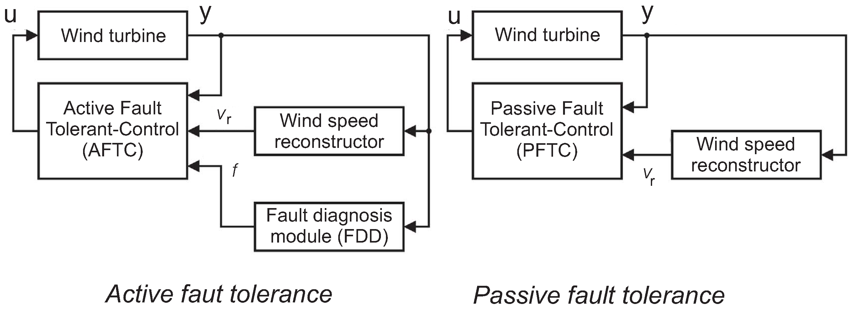
The two basic sustainable control solutions have different structures, as shown in Figure 14. Note that only the active fault-tolerant controller (AFTC) relies on a fault diagnosis algorithm (FDD). This represents the main difference between the two control schemes.

The main point between AFTC and PFTC schemes is that an active fault-tolerant controller relies on a fault diagnosis system, which provides information about the faults f to the controller [51]. In the considered case the fault diagnosis system FDD contains the estimation of the unknown input (fault) affecting the system under control. The knowledge of the fault f allows the AFTC to reconfigure the current state of the system. On the other hand, the FDD is able to improve the controller performance in fault-free conditions, since it can compensate e.g., the modelling errors, uncertainty and disturbances. On the other hand, the PFTC scheme does not rely on a fault diagnosis algorithm, but is designed to be robust towards any possible faults. This is accomplished by designing a controller that is optimised for the fault-free situation, while satisfying some graceful degradation requirements in the faulty cases. However, with respect to the robust control design, the PFTC strategy provides reliable controllers that guarantee the same performance with no risk of false FDI or reconfigurations [51].

Figure 14. Sustainable control systems.

Figure 14. Sustainable control systems.

In general, the methods used in the fault-tolerant controller designs should rely on output feedback, since only part of the state vector is measured. Additionally, they should take the measurement noise into account. Moreover, the design methods should be suited for nonlinear systems or linear systems with varying parameters. The latest proposed solutions for the derivation of both active and the passive fault-tolerant controllers rely on LPV and fuzzy descriptions, to which the fault-tolerance properties are added, since these frameworks methods are able to provide stability and guaranteed performance with respect to parameter variations, uncertainty and disturbance. Additionally, LPV and fuzzy controller design methods have been recently proposed and evaluated for wind turbine application [4,15]. To add fault-tolerance to the basic controller formulations outlined in Section 4, different approaches can be exploited. For example, the AFTC scheme can use the parameters of suitable model structures estimated by the FDD module for scheduling the controllers [4,15]. On the other hand, different approaches can be used to obtain fault-tolerance in the PFTC methods. For this purpose, the design methods described in [15,34] can be modified to cope with parametric uncertainties, as addressed e.g., in [13,14,52,53]. Alternatively, other methods could have been used such as [54], which preserves the nominal performance. Generally, these approaches rely on solving some optimisation problems where a controller is calculated subject to maximising the disturbance attenuation, using Linear Matrix Inequality (LMI) tools [14,55].

6. Conclusions

This paper analysed the most important modelling and control issues of wind turbines from system and control engineering points of view. A walk around the wind turbine control loops discussed the goals of the most common solutions and overviews the typical actuation and sensing available on commercial turbines. The work also intended to provide an updated and broader perspective by covering not only the modelling and control of individual wind turbines, but also outlining a number of areas for further research, and anticipating new issues that can open up new paradigms for advanced control approaches. In summary, wind energy is a fast growing industry, and this growth has led to a large demand for better modelling and control of wind turbines. Uncertainty, disturbance and other deviations from normal working conditions of the wind turbines make the control challenging, thus motivating the need for advanced modelling and a number of so-called sustainable control approaches that should be explored to reduce the cost of wind energy. By enabling this clean renewable energy source to provide and reliably meet the world’s electricity needs, the tremendous challenge of solving the world’s energy requirements in the future will be enhanced. The wind resource available worldwide is large, and much of the world’s future electrical energy needs can be provided by wind energy alone if the technological barriers are overcome. The application of sustainable controls for wind energy systems is still in its infancy, and there are many fundamental and applied issues that can be addressed by the systems and control community to significantly improve the efficiency, operation, and lifetimes of wind turbines.

References

- Johnson, K.E.; Fleming, P.A. Development, implementation, and testing of fault detection strategies on the National Wind Technology Center’s controls advanced research turbines. Mechatronics 2011, 21, 728–736. [Google Scholar] [CrossRef]
- Global Wind Energy Council. Wind Energy Statistics 2014; Global Wind Energy Council: Brussels, Belgium, 10 February 2015. [Google Scholar]
- Burton, T.; Sharpe, D.; Jenkins, N.; Bossanyi, E. Wind Energy Handbook, 2nd ed.; John Wiley & Sons: New York, NY, USA, 2011. [Google Scholar]
- Odgaard, P.F.; Stoustrup, J.; Kinnaert, M. Fault-tolerant control of wind turbines: A benchmark model. IEEE Trans. Control Syst. Technol. 2013, 21, 1168–1182. [Google Scholar] [CrossRef]
- David Rivkin, D.; Anderson, L.D.; Silk, L. Wind Turbine Control Systems, 1st ed.; Jones & Bartlett Learning: Burlington, MA, USA, 2012. [Google Scholar]
- Bianchi, F.D.; Battista, H.D.; Mantz, R.J. Advances in industrial control. In Wind Turbine Control Systems: Principles, Modelling and Gain Scheduling Design, 1st ed.; Springer-Verlag: Berlin, Germany, 2007. [Google Scholar]
- Garcia-Sanz, M.; Houpis, C.H. Wind Energy Systems: Control Engineering Design; CRC (Chemical Rubber Company) Press: Boca Raton, FL, USA, 2012. [Google Scholar]
- Ningsu, L.; Vidal, Y.; Acho, L. Advances in industrial control. In Wind Turbine Control and Monitoring; Springer-Verlag: Berlin Heidelberg, Germany, 2014. [Google Scholar]
- Blanke, M.; Kinnaert, M.; Lunze, J.; Staroswiecki, M. Diagnosis and Fault-Tolerant Control; Springer-Verlag: Berlin Heidelberg, Germany, 2006. [Google Scholar]
- Ding, S.X. Model-based Fault Diagnosis Techniques: Design Schemes, Algorithms, and Tools, 1st ed.; Springer-Verlag: Berlin Heidelberg, Germany, 2008. [Google Scholar]
- Isermann, R. Fault-Diagnosis Systems: An Introduction from Fault Detection to Fault Tolerance, 1st ed.; Springer-Verlag: Berlin Heidelberg, Germany, 2005. [Google Scholar]
- Pao, L.Y.; Johnson, K.E. Control of wind turbines. IEEE Control Syst. Mag. 2011, 31, 44–62. [Google Scholar] [CrossRef]
- Schulte, H.; Gauterin, E. Fault-tolerant control of wind turbines with hydrostatic transmission using takagi-sugeno and sliding mode techniques. Annu. Rev. Control 2015, 12. [Google Scholar] [CrossRef]
- Shi, F.; Patton, R.J. An active fault tolerant control approach to an offshore wind turbine Model. Renew. Energy 2015, 75, 788–798. [Google Scholar] [CrossRef]
- Odgaard, P.F.; Stoustrup, J. A benchmark evaluation of fault tolerant wind turbine control concepts. IEEE Trans. Control Syst. Technol. 2015, 23, 1221–1228. [Google Scholar] [CrossRef]
- Jonkman, J.M.; Buhl, M.L., Jr. FAST User’s Guide; Technical Report NREL/EL-500-38230; National Renewable Energy Laboratory: Golden, CO, USA, 2005. [Google Scholar]
- Jonkman, J.; Butterfield, S.; Musial, W.; Scott, G. Definition of a 5-MW Reference Wind Turbine for Offshore System Development; Technical Report NREL/TP-500-38060; National Renewable Energy Laboratory: Golden, CO, USA, 2009. [Google Scholar]
- Gasch, R.; Twele, J. Wind Power Plants: Fundamentals, Design, Construction and Operation, 2nd ed.; Springer-Verlag: Berlin Heidelberg, Germany, 2012. [Google Scholar]
- Georg, S.; Schulte, H.; Aschemann, H. Control-oriented modelling of wind turbines using a Takagi-Sugeno model structure. In Proceedings of the IEEE International Conference on Fuzzy Systems, Brisbane, Australia, 10–15 June 2012; pp. 1737–1744.
- Landau, L.D.; Lifshitz, E.M. Course of theoretical physics S. In Mechanics, 3rd ed.; Butterworth-Heinemann: Waltham, MA, USA, 1976; Volume 1. [Google Scholar]
- Laino, D.J.; Hansen, A.C. Windward engineering, LC. In User’s Guide to the Wind Turbine Aerodynamics Computer Software AeroDyn; Technical Report TCX-9-29209-01; Windward Engineering: Salt Lake City, UT, USA, 2002. [Google Scholar]
- Heier, S. Grid Integration of Wind Energy: Onshore and Offshore Conversion Systems, 3rd ed.; John Wiley & Sons: Hoboken, NJ, USA, 2014. [Google Scholar]
- Simani, S.; Castaldi, P. Estimation of the power coefficient map for a wind turbine system. In Proceedings of the 9th European Workshop on Advanced Control and Diagnosis—ACD 2011, Budapest, Hungary, 17–18 November 2011.
- Simani, S.; Castaldi, P. Active actuator fault tolerant control of a wind turbine benchmark model. Int. J. Robust Nonlinear Control 2014, 24, 1283–1303. [Google Scholar]
- Odgaard, P.F.; Stoustrup, J. Fault tolerant wind farm control—A benchmark model. In Proceedings of the IEEE Multiconference on Systems and Control—MSC2013, Florence, Italy, 10–13 December 2013; pp. 1–6.
- Odgaard, P.F.; Johnson, K. Wind turbine fault diagnosis and fault tolerant control—An enhanced benchmark challenge. In Proceedings of the 2013 American Control Conference—ACC, IEEE Control Systems Society & American Automatic Control Council, Chicago, IL, USA, 1–3 July 2013; pp. 4447–4452.
- Simani, S.; Farsoni, S.; Castaldi, P. Fault diagnosis of a wind turbine benchmark via identified fuzzy models. IEEE Trans. Ind. Electr. 2014, 62, 3775–3782. [Google Scholar] [CrossRef]
- Simani, S.; Farsoni, S.; Castaldi, P. Wind turbine simulator fault diagnosis via fuzzy modelling and identification techniques. Sustain. Energy Grids Netw. 2015, 1, 45–52. [Google Scholar] [CrossRef]
- Bossanyi, E.A.; Hassan, G. The design of closed loop controllers for wind turbines. Wind Energy 2000, 3, 149–164. [Google Scholar] [CrossRef]
- Bossanyi, E.A. Wind turbine control for load reduction. Wind Energy 2003, 6, 229–244. [Google Scholar] [CrossRef]
- Betz, A.; Randall, D.G. Introduction to the Theory of Flow Machines; Permagon Press: Oxford, UK, 1966. [Google Scholar]
- Chatzopoulos, A.P.; Leithead, W.E. Reducing tower fatigue loads by a co-ordinated control of the Supergen 2 MW exemplar wind turbine. In Proceedings of the 3rd Torque 2010 Conference, Crete, Greece, 28–30 June 2010; pp. 667–674.
- Odgaard, P.F. FDI/FTC wind turbine benchmark modelling. In Workshop on Sustainable Control of Offshore Wind Turbines; Patton, R.J., Ed.; Centre for Adaptive Science & Sustainability, University of Hull: Hull, UK, 2012; Volume 1. [Google Scholar]
- Simani, S.; Castaldi, P. Data-driven and adaptive control applications to a wind turbine benchmark model. Control Eng. Pract. 2013, 21, 1678–1693. [Google Scholar] [CrossRef]
- Simani, S.; Castaldi, P. Identification-oriented control designs with application to a wind turbine benchmark. Int. J. Adv. Comput. Sci. Appl. 2013, 4, 184–191. [Google Scholar] [CrossRef]
- Johnson, K.E.; Pao, L.Y.; Balas, M.J.; Fingersh, L.J. Control of variable-speed wind turbines: Standard and adaptive techniques for maximizing energy capture. IEEE Control Syst. Mag. 2006, 26, 70–81. [Google Scholar] [CrossRef]
- Munteanu, I.; Bratcu, A.I. Advances in industrial control. In Optimal Control of Wind Energy Systems: Towards a Global Approach; Springer-Verlag: Berlin Heidelberg, Germany, 2008. [Google Scholar]
- Amit Dixit, A.; Suryanarayanan, S. Towards pitch-scheduled drivetrain damping in variable-speed, horizontal-axis large wind turbines. In Proceedings of 44th IEEE Conference on Decision and Control, Plaza de Espana Seville, Spain, 12–15 December 2005; pp. 1295–1300.
- Wright, A.; Fingersh, L.; Balas, M. Testing state-space controls for the controls of advanced research turbine. ASME J. Sol. Energy Eng. 2006, 128, 506–515. [Google Scholar] [CrossRef]
- Laks, J.H.; Pao, L.Y.; Wright, A.D. Control of wind turbines: Past, present, and future. In Proceedings of the American Control Conference, 2009—ACC’09, St. Louis, MO, USA, 10–12 June 2009; pp. 2096–2103.
- Kumar, A.; Stol, K. Scheduled model predictive control of a wind turbine. In Proceedings of the 47th AIAA (American Institute of Aeronautics and Astronautics) Wind Energy Symposium, Orlando, FL, USA, 7–10 January 2009; pp. 1–18.
- Laks, J.; Pao, L.Y.; Simley, E.; Wright, A.; Kelley, N.; Jonkman, B. Model predictive control using preview measurements from LIDAR. In Proceedings of the 49th AIAA (American Institute of Aeronautics and Astronautics) Wind Energy Symposium, Orlando, FL, USA, 4–7 January 2011; pp. 1–20.
- Kumar, A.; Stol, K. Simulating feedback linearization control of wind turbines using high-order models. Wind Energy 2010, 13, 419–432. [Google Scholar] [CrossRef]
- Burkart, R.; Margellos, K.; Lygeros, J. Nonlinear control of wind turbines: An approach based on switched linear systems and feedback linearization. In Proceedings of the 50th IEEE Conference on Decision and Control and European Control Conference (CDC-ECC), Orlando, FL, USA, 12–15 December 2011; pp. 5485–5490.
- Boukhezzar, B.; Lupu, L.; Siguerdidjane, H.; Hand, M. Multivariable control strategy for variable speed, variable pitch wind turbines. Renew. Energy 2007, 32, 1273–1287. [Google Scholar] [CrossRef]
- Thomsen, S.C.; Niemann, H.; Poulsen, N.K. Individual pitch control of wind turbines using local inflow measurements. In Proceedings of the 17th IFAC (The International Federation of Automatic Control) World Congress, Seoul, Korea, 6–11 July 2008; pp. 5587–5592.
- Friis, J.; Nielsen, E.; Bonding, J.; Adegas, F.D.; Stoustrup, J.; Odgaard, P.F. Repetitive model predictive approach to individual pitch control of wind turbines. In Proceedings of the IEEE Conference on Decision and Control and European Control Conference (CDC & ECC), Orlando, FL, USA, 12–15 December 2011; pp. 3664–3670.
- McCoy, T.J.; Griffin, D.A. Control of rotor geometry and aerodynamics: Retractable blades and advanced concepts. Wind Eng. 2009, 32, 13–26. [Google Scholar] [CrossRef]
- Gong, X.; Qiao, W. Bearing fault diagnosis for direct-drive wind turbines via current–demodulated signals. IEEE Trans. Ind. Electr. 2013, 60, 3419–3428. [Google Scholar] [CrossRef]
- Freire, N.M.A.; Estima, J.O.; Marques Cardoso, A.J. Open-circuit fault diagnosis in PMSG drives for wind turbine applications. IEEE Trans. Ind. Electr. 2013, 60, 3957–3967. [Google Scholar] [CrossRef]
- Mahmoud, M.; Jiang, J.; Zhang, Y. Lecture notes in control and information sciences. In Active Fault Tolerant Control Systems: Stochastic Analysis and Synthesis; Springer-Verlag: Berlin, Germany, 2003. [Google Scholar]
- Rodrigues, M.; Theilliol, D.; Aberkane, S.; Sauter, D. Fault tolerant control design for polytopic LPV systems. Int. J. Appl. Math. Comput. Sci. 2007, 17, 27–37. [Google Scholar] [CrossRef]
- Puig, V. Fault diagnosis and fault tolerant control using set-membership approaches: application to real case studies. Int. J. Appl. Math. Comput. Sci. 2010, 20, 619–635. [Google Scholar] [CrossRef] [Green Version]
- Niemann, H.; Stoustrup, J. An architecture for fault tolerant controllers. Int. J. Control 2005, 78, 1091–1110. [Google Scholar] [CrossRef]
- Chen, Z.; Patton, R.J.; Chen, J. Robust fault-tolerant system synthesis via LMI. In Proceedings of the IFAC Symposium on Fault Detection, Supervision and Safety for Technical Processes: SAFEPROCESS’97, Hull, UK, 26–28 August 1997; Volume 1, pp. 347–352.
© 2015 by the author; licensee MDPI, Basel, Switzerland. This article is an open access article distributed under the terms and conditions of the Creative Commons by Attribution (CC-BY) license (http://creativecommons.org/licenses/by/4.0/).
Share and Cite
MDPI and ACS Style
Simani, S. Overview of Modelling and Advanced Control Strategies for Wind Turbine Systems. Energies 2015, 8, 13395-13418. https://doi.org/10.3390/en81212374
AMA Style
Simani S. Overview of Modelling and Advanced Control Strategies for Wind Turbine Systems. Energies. 2015; 8(12):13395-13418. https://doi.org/10.3390/en81212374
Chicago/Turabian StyleSimani, Silvio. 2015. "Overview of Modelling and Advanced Control Strategies for Wind Turbine Systems" Energies 8, no. 12: 13395-13418. https://doi.org/10.3390/en81212374