Article

General Dynamic Equivalent Modeling of Microgrid Based on Physical Background

1
Jiangsu Key Laboratory of Power Transmission & Distribution Equipment Technology, Hohai University, Changzhou 213022, Jiangsu, China
2
College of IOT Engineering, Hohai University, Changzhou 213022, Jiangsu, China
3
Changzhou Key Laboratory of Photovoltaic System Integration and Production Equipment, Hohai University, Changzhou 213022, Jiangsu, China
*
Author to whom correspondence should be addressed.
Energies 2015, 8(11), 12929-12948; https://doi.org/10.3390/en81112354
Submission received: 17 September 2015 / Revised: 14 October 2015 / Accepted: 9 November 2015 / Published: 17 November 2015
(This article belongs to the Special Issue Electric Power Systems Research)

Abstract

:
Microgrid is a new power system concept consisting of small-scale distributed energy resources; storage devices and loads. It is necessary to employ a simplified model of microgrid in the simulation of a distribution network integrating large-scale microgrids. Based on the detailed model of the components, an equivalent model of microgrid is proposed in this paper. The equivalent model comprises two parts: namely, equivalent machine component and equivalent static component. Equivalent machine component describes the dynamics of synchronous generator, asynchronous wind turbine and induction motor, equivalent static component describes the dynamics of photovoltaic, storage and static load. The trajectory sensitivities of the equivalent model parameters with respect to the output variables are analyzed. The key parameters that play important roles in the dynamics of the output variables of the equivalent model are identified and included in further parameter estimation. Particle Swarm Optimization (PSO) is improved for the parameter estimation of the equivalent model. Simulations are performed in different microgrid operation conditions to evaluate the effectiveness of the equivalent model of microgrid.

1. Introduction

In order to increase the reliability of the electricity supply to the sensitive load, microgrid concept was proposed and developed in recent years [1,2]. Microgrid normally consists of distributed energy resources (DER), energy storage devices and loads. Most of the time, microgrid can be regarded as a self-controlled system that separates and isolates itself from the utility when a severe disturbance nearby occurs, and reconnects itself to the grid automatically when the disturbance is cleared. Obviously, the operational characteristics of the microgrid are quite different from those of the traditional electrical equivalent. Hence, the increasing penetration of the microgrid will have significant impact on the dynamic performances of the distribution network.
To investigate the interactive effect between microgrid and distribution network, a suitable microgrid model is needed. The detailed model of the microgrid comprises dozens of differential equations of all dynamic and static components [2,3,4]. In a simple distribution network with a small number of microgrids, the detailed model of the microgrid is suitable for the dynamic simulation of the distribution network when the microgrid under connected operation mode [5]. However, with increasing penetration of the microgrid into the distribution network, the simulation of a large-scale distribution network becomes very difficult. Under this condition, if an equivalent model of the microgrid is employed, the simulation of the distribution network can be simplified.
Microgrid should operate under connected mode most time to take full advantages of distributed generator. Compared with the distribution network, microgrid can be seen as a controlled load or a controlled electric source under this operation mode. In connected mode, the interactions between loads and distributed generations can be ignored, and the microgrid synthesized dynamic characteristics will be considered in the simulation of distribution network.
Distributed generation is the basis of microgrid; if the equivalent model of the distributed generation is utilized, dynamic simulation of the microgrid can be simplified. An equivalent model compared with the detailed model of the photovoltaic was discussed in [6], and the equivalent model could well describe the dynamic characteristics of the photovoltaic under different faults in power grid. The authors of [7,8] proposed a photovoltaic source dynamic model, the parameters of which were identified based on a least-squares regression-based data processing algorithm. The singular perturbations theory was applied to reduce the model order of the wind farm in [9], and the dynamics of the reduced-order model matched well with those of the detailed model under different operational conditions. Aggregate modeling and detailed modeling for the transient interaction between a large wind farm and a power system were discussed in [10], and the aggregate modeling decreased the simulation time without significantly compromising the accuracy in different conditions. In [11,12], an equivalent method was proposed for integrating wind power generation system in power flow and transient simulation, the unit plants equivalent method and the multiply equivalent method were used for the power flow calculation and transient dynamics simulation, respectively. A probabilistic clustering concept for aggregate modeling of wind farms was proposed in [13], the support vector clustering technique was used to cluster wind turbines based on wind farm layout and incoming wind. Due to the short distances of the electric circuits in the microgrid, there is a strong electromagnetic coupling between the electrical components. These characteristics increase the difficulty in the microgrid analysis. A generalized homology equivalence theory based on differential geometry was used for the microgrid equivalent modeling in [14], and the mathematical analysis of its reduced-order nature was discussed.
Parameter estimation method is a very difficult and challenging task in system modeling. Recently, global optimization techniques such as genetic algorithm [15], evolutionary algorithm [16] and differential evolution [17] have been proposed to solve the parameter estimation problems. Though the genetic algorithm (GA) was employed successfully to solve complex non-linear optimization problems, some deficiencies of GA have been identified in recent research [18]. This degradation in efficiency is apparent when the parameters being optimized are highly correlated and the premature convergence of the GA degrades its performance in terms of reducing the search capability.
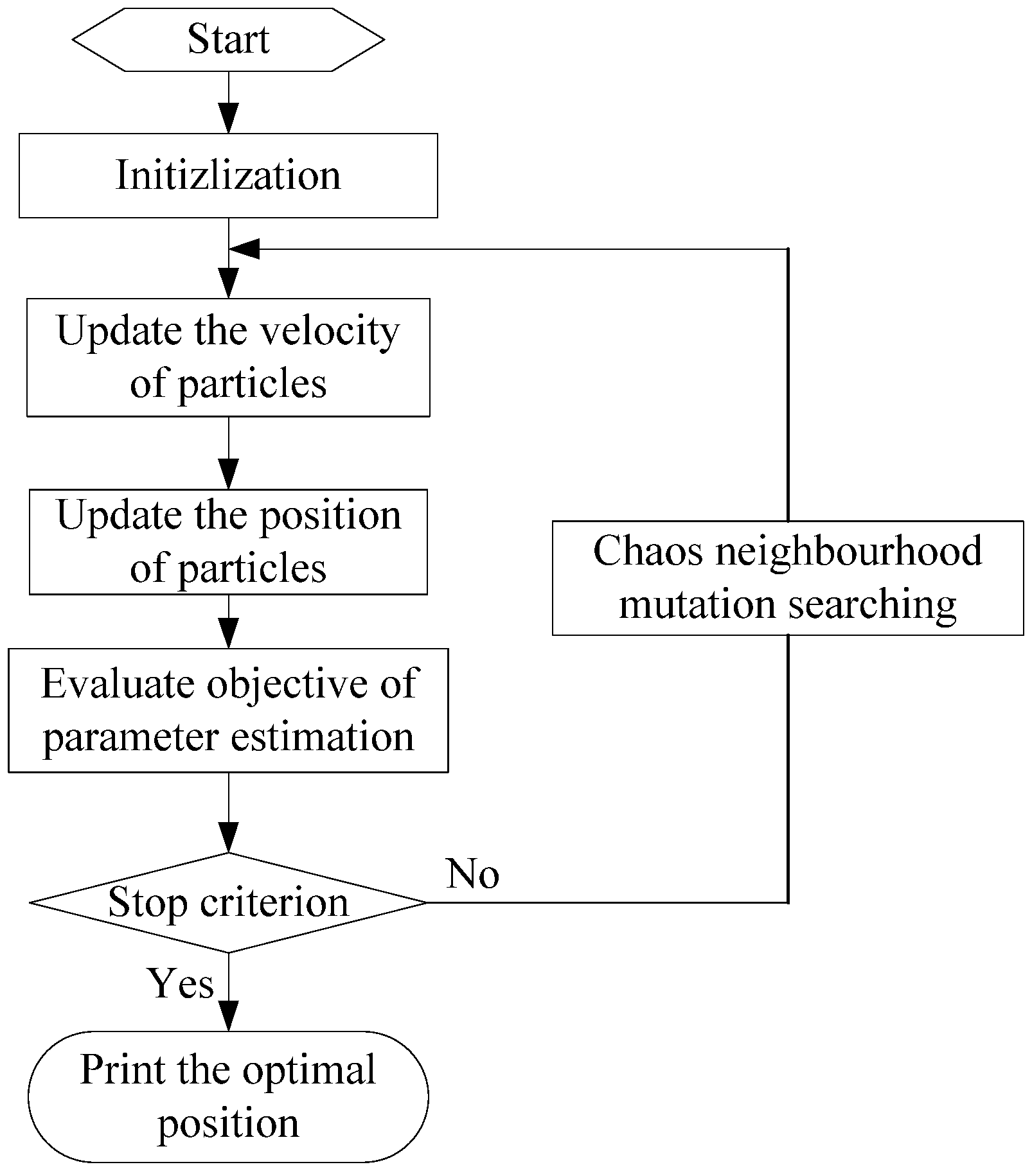
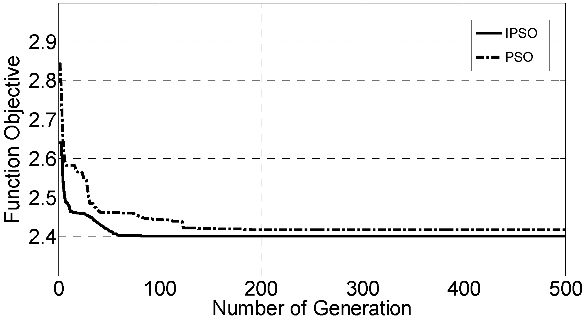
Particle swarm optimization (PSO) is an evolutionary computation technique in nature motivated by the simulation of social behaviors. In searching the optimal solution of a problem, information of the best position of each individual particle and the best position among the whole swarm are used to direct the searching. Due to the simple concept, easy implementation and quick convergence, nowadays PSO has gained much attention and wide applications in different fields. Authors of papers [19,20,21,22,23,24] showed that PSO is a feasible approach to parameter estimation of nonlinear systems. In [19], PSO was applied in harmonic estimation. A modified PSO was utilized in the maximum power point tracking for the photovoltaic system in [20]. In the field of parameter estimation, PSO-based parameter estimation technique of proton exchange membrane fuel cell models was proposed in [21], and PSO with quantum was introduced successfully in synchronous generator offline and online parameters estimation problem. Parameter estimation of an induction machine using PSO was shown in [22], and the dynamic PSO and chaos PSO were better than the standard PSO. PSO was used for jointly estimating both the parameters and states of the lateral flow immunoassay model in [23]. Diffusion particle swarm optimization was proposed to optimize the maximum likelihood function in [24], and the PSO technique has been shown to provide a good solution to bearing estimation as it alleviates the effects of multi-modality.
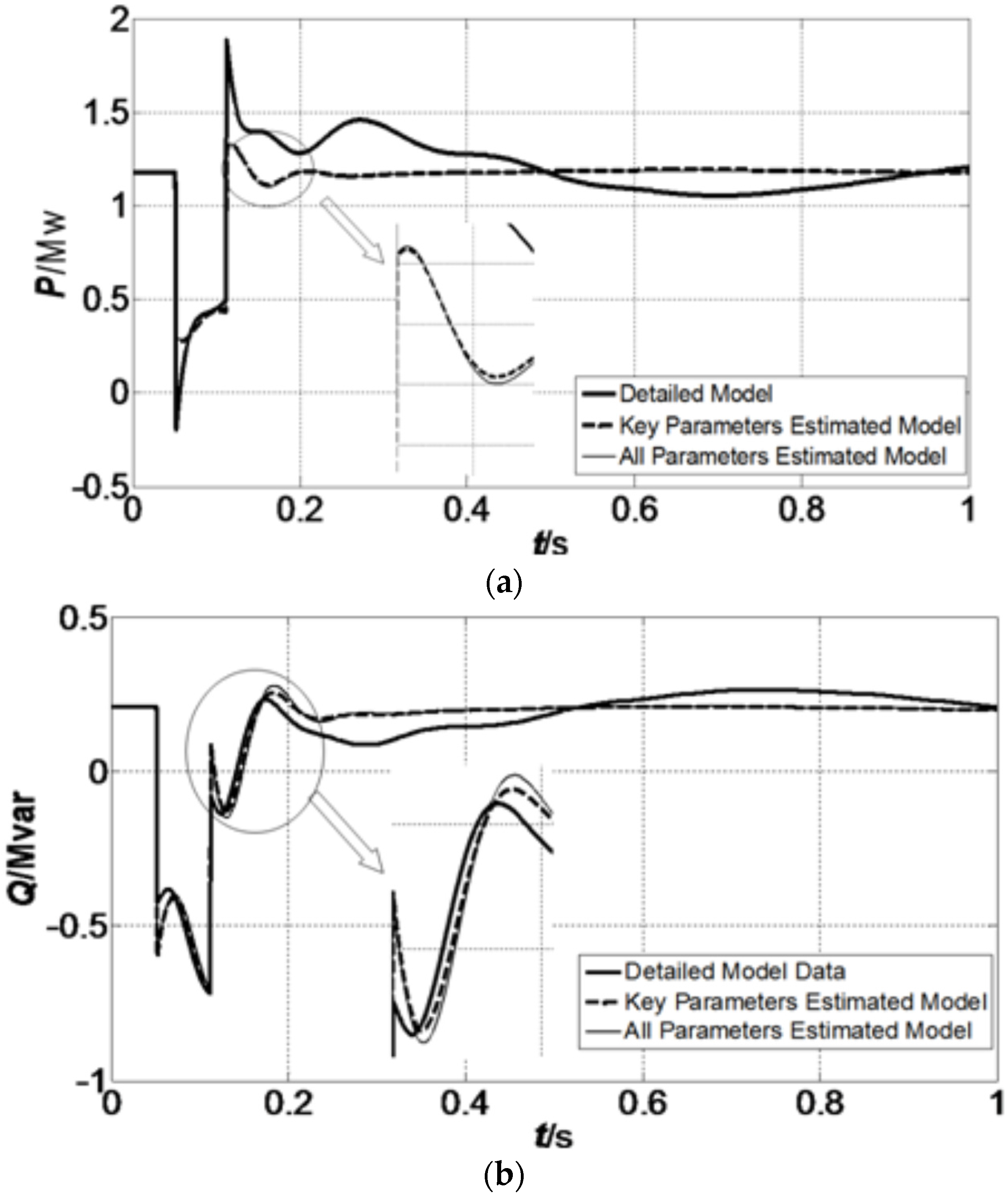
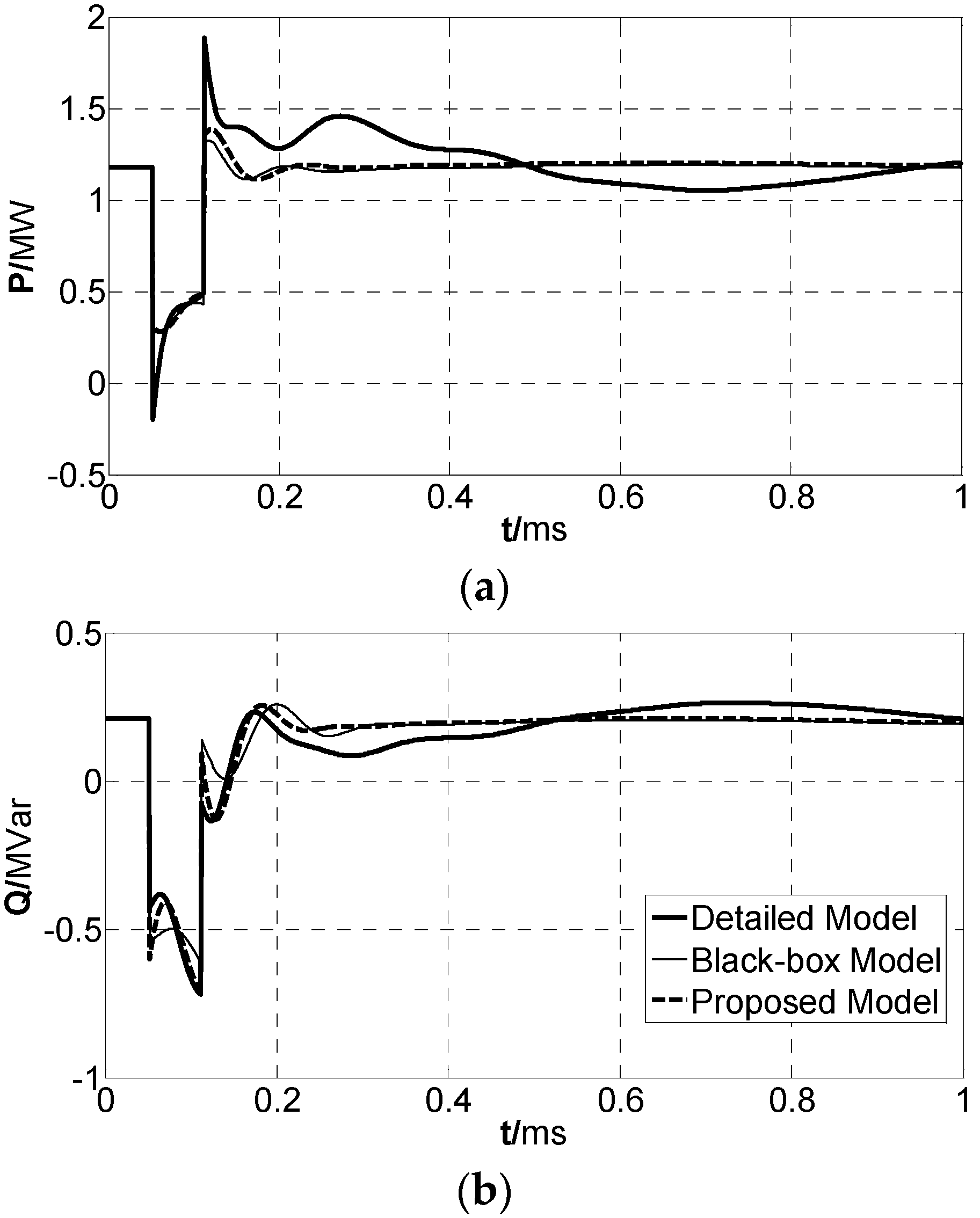
Research has been carried out in the fields of detailed modeling of microgrid and equivalent modeling of the distributed generation. With the increasing penetration of microgrids, the interaction between the microgrid and the distribution network should not be ignored in the power system real-time simulation. However, this will increase the complexity of the simulation with the detailed model of the microgrid components. Hence, a simplified equivalent model of the microgrid is extremely urgent for the simulation analysis of the distribution network. Based on the component detailed models and synthetically dynamic characteristics of the microgrid, an equivalent model of microgrid is proposed in this paper. The proposed equivalent model contains two parts: equivalent static component and equivalent machine component. In order to increase the accuracy of the parameters estimation, trajectory sensitivity is used to identify the key parameters for the further steps of parameter estimation. Particle Swarm Optimization (PSO) is improved and employed to estimate the parameters of the equivalent model. The presented equivalent model and modeling method are shown to be effective by the simulation study on a microgrid connected into distribution network.

2. Microgrid Equivalent Model

A microgrid is made up of a large number of distribution generations, electrical loads and storage devices. Typically, there are two types of components: static components and rotating machines [1]. Static components contain photovoltaic (PV) and static loads. It is common that PV connects to the microgrid through power electronics equipment. Maximum Point Power Tracking (MPPT) and constant power control strategy are applied to the power electronics equipment when the microgrid is connected in the grid-connected operation mode [25]. The output power of these distribution generations is controllable and the dynamic characteristics of them are similar with the static load. In principle, the static load is represented by an exponential of the voltage and frequency [26]. Hence, the output power of the static components can be described by an exponential of the voltage and frequency.
Rotating machine components contain induction motor load, asynchronous induction wind generator and synchronous generator. The structure and the mathematical equations of the asynchronous induction wind generator are similar with those of the induction motor load [27]. The synchronous machine generator and the asynchronous wind generator have similar dynamic characteristics during faults, and the only difference between them is the modeling reference frames. The synchronous machine rotor angular velocity is constant and the velocity voltage is zero in steady-state conditions [28]. However, the rotor angular velocity of synchronous will deviate slightly from the synchronous velocity during a fault since the synchronous machine capability is small in most microgrids. The rotor angular velocity is not equal to the system synchronous velocity and its electrical structure is similar with that of the asynchronous induction wind generator, so the synchronous machine generator can be regarded as an asynchronous machine generator during a fault. Furthermore, the synchronous machine generator, the asynchronous induction wind generator and the induction motor load can be described with a unified mathematical model in the transient dynamic analysis.
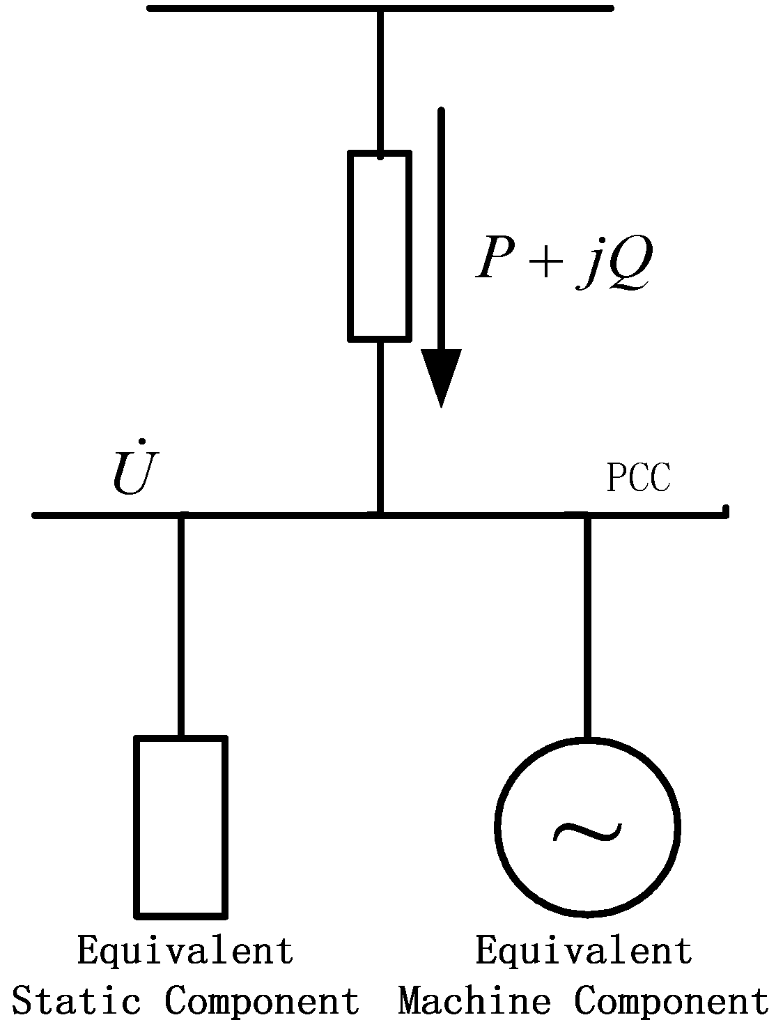
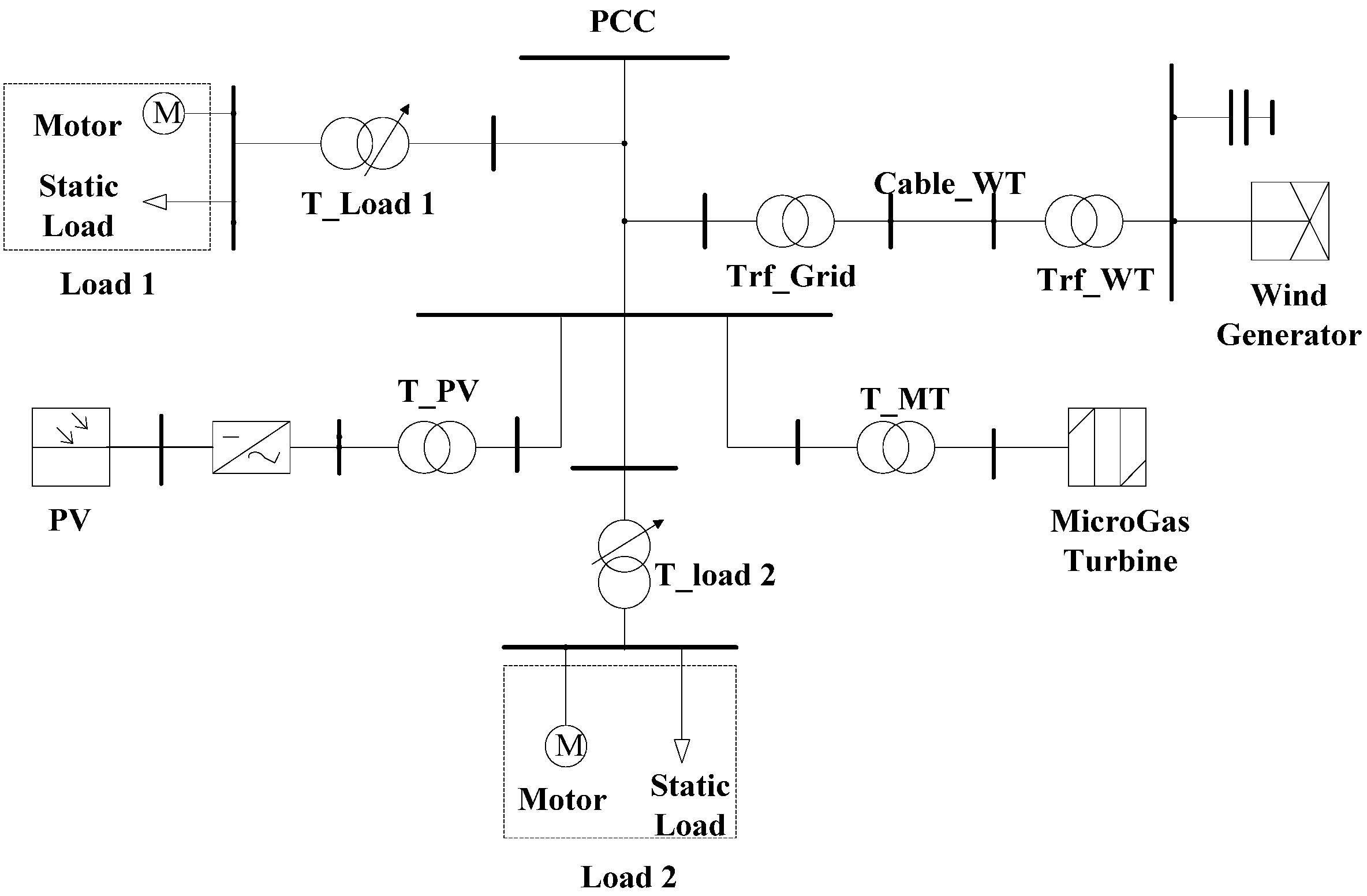
As shown in Figure 1, the equivalent model of the microgrid is comprised of an equivalent static component and an equivalent machine component. The equivalent static component is parallel to the equivalent machine component, and they are connected to the distribution network through the Point of Coupling Common (PCC).

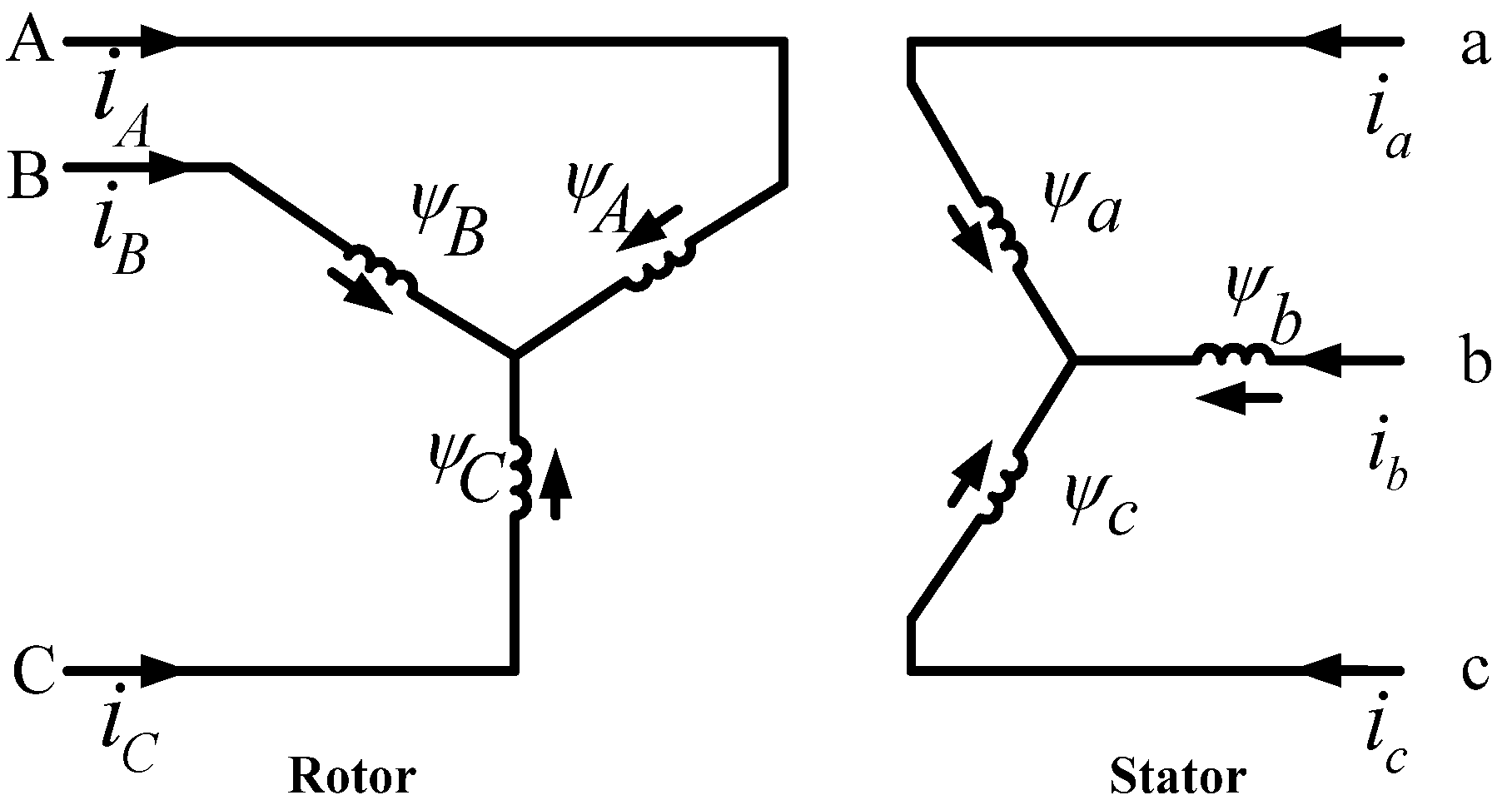
2.1. Equivalent Machine Component

The stator and rotor circuits of the equivalent machine component are shown in Figure 2.
Rotor angular velocity ω r is different from the stator angular velocity ω s . Applying d q 0 transformation [29], stator voltage equations can be written as
u d s = p ψ d s ω s ψ q s r s i d s u q s = p ψ q s + ω s ψ d s r s i q s
Figure 1. The equivalent model of microgrid.
Energies 08 12354 g001
Figure 2. Equivalent circuit of the equivalent machine component.
Energies 08 12354 g002
Rotor voltage equations can be written as
u d r = p ψ d r ω s s ψ q r + r d r i d r u q r = p ψ q r + ω s s ψ d r + r q r i q r
where u d s and u q s are the stator voltages; ψ d s and ψ q s are the stator flux linkages; r s is stator resistance; i d s and i q s are stator currents; u d r and u q r are rotor voltages; ψ d r and ψ q r are rotor flux linkages; r d r and r q r are rotor resistance; i d r and i q r are rotor currents; s = ω s ω r ω s is the rotor slip; and p = d d t is the per time derivative.
The stator flux linkage is
ψ d s = L d s i d s + L a d i d r ψ q s = L q s i q s + L a q i q r
The rotor flux linkage is
ψ d r = L a d i d s + L d r i d r ψ q r = L a q i q s + L q r i q r
where L d s and L q s are the stator inductances; L d r and L q r are the rotor inductances; and L a d and L a q are mutual inductances.
Using the definitions below:
L d = L d s L a d 2 L d r , L q = L q s L a q 2 L q r T d 0 = L d r r d r , T q 0 = L q r r q r E d = L a q L d r ψ d r , E q = L a d L q r ψ q r E d r = L a d L d r u d r , E q r = L a q L q r u q r
rotor voltage equations may be rewritten as follows:
d E d d t = E d r + ω s s L d r L a d L a q L q r E q 1 T q 0 ( E d + ( L q s L q ) i q s ) d E q d t = E q r ω s s L q r L a q L a d L d r E d 1 T d 0 ( E q ( L d s L d ) i d s )
When representing power system stability studies, p ψ d s and p ψ q s are neglected in the stator voltage relations. Their neglect corresponds to ignoring the dc component in the stator transient currents, permitting representation of only fundamental frequency components [28]. With the stator transients neglected, stator voltage equations may be rewritten as:
u d s = ω s [ ( L q s L a q 2 L q r ) i q s + L a q L q r ψ q r ] + r s i d s u q s =     ω s [ ( L d s L a d 2 L d r ) i d s + L a d L d r ψ d r ] + r s i q s
From Equations (5) and (7), we have
u d s = r s i d s ω s L q i q s + ω s E d u q s = r s i q s + ω s L d i d s + ω s E q
The rotor acceleration equation, with time expressed in seconds, is
d ω r d t = 1 T j ( T M T e )
where T e is the electromagnetic torque, T M is the mechanical torque, and T j is the inertia constant of the rotor. Eliminating the rotor currents by expressing them in terms of the stator currents and rotor flux linkages, we find that the per unit electromagnetic torque is
T e = ψ q r i d r ψ d r i q r = E q i q s E d i d s ( ω s L d ω s L q ) i d s i q s
The system frequency of the microgrid is constant when the microgrid operation in connected mode. Thus, rotor acceleration equation with f = ω s = 1 pu can be written as:
d ω r d t = 1 T j [ T M ( E q i q s E d i d s ( L d L q ) i d s i q s ) ]
The output active power and reactive power of the equivalent machine component may be written as:
P m = u d s i d s u q s i q s Q m = u q s i d s u d s i q s

2.2. Equivalent Static Component

Static load model represents the load characteristics as an algebraic function of the bus voltage magnitude and frequency [26]. Equivalent static component, including static load and distribution generation such as PV in microgrid, is described using algebraic equations. The active and reactive power of the equivalent static component model are related to the system voltage and frequency in the following form:
P s = P s 0 ( U / U 0 ) p u ( f / f 0 ) p f Q s = Q s 0 ( U / U 0 ) q u ( f / f 0 ) q f
where P s and Q s are the active and reactive power of the equivalent static component when the voltage magnitude is U and frequency is f , respectively. The subscript 0 identifies the values of the respective variables at the initial operating condition of PCC. The parameters of this model are the exponents p u , q u , p f and q f , where p u is the coefficient of the active power and voltage, p f is the coefficient of active power and frequency, q u is the coefficient of reactive power and voltage, and q f is the coefficient of reactive power and frequency.
The system frequency of the microgrid is constant when the microgrid operates in grid-connected mode. Thus, with f = 1 pu, the model of the equivalent static component can be written as:
P s = P s 0 ( U / U 0 ) p u Q s = Q s 0 ( U / U 0 ) q u

2.3. Parameters of the Equivalent Model

From model Equations (6), (8), (11), (12) and (14), it can be seen that the equivalent model parameters include r s , L d s , L q s , L d , L q , L d r , L q r , L a d , L a q , T d 0 , T q 0 , T j , p u , and q u . In order to describe the physical characteristics of the equivalent model, the equivalent model parameters are initialized with corresponding fundamental parameters and will be further estimated in the microgrid modeling. Based on the definitions of the parameters in Equation (5), the fundamental parameters of the equivalent machine component are r s , L s l , L a d , L a q , r d r , L d r l , r q r , L q r l , T j , p u , and q u , where L s l is the stator leakage inductance; L a d and L a q are mutual inductances of d and q axis; r d r and r q r are rotor resistances of d and q axis; and L d r l and L q r l are rotor leakage inductances of d and q axis.
There are other two important parameters, namely s 0 and K m p . Where s 0 is the initial slip of the equivalent machine component, and s 0 presents the type of equivalent machine. If s 0 > 0 , the equivalent machine component absorbs power from the distribution network, and has the characteristics of induction motor load. Oppositely, s 0 < 0 means that the equivalent machine component injects power into the distribution network, and has the characteristics of asynchronous generator. K m p is the fraction of the equivalent machine component active power with respect to the total initial active power P . The active power flow between the microgrid and the distribution network is bidirectional. Thus, P > 0 indicates that the microgrid absorbs power from the distribution network, and P < 0 indicates that the microgrid injects power into the distribution network. The similar definition is also applied to reactive power Q.
As a result, the 13 parameters, namely K m p , s 0 , r s , L s l , L a d , L a q , r d r , L d r l , r q r , L q r l , T j , p u , and q u , in the equivalent microgrid model need to be estimated in the microgrid equivalent dynamic modeling.

3. Equivalent Model Parameter Sensitivity Analysis

The number of the parameters to be estimated has significant impact on the accuracy of the parameters estimation. Parameter sensitivity analysis is an efficient method to determine the key parameters of the equivalent model. Parameter trajectory sensitivity is defined as:
y ( θ , k ) θ j = lim Δ θ j 0 y ( θ 1 , , θ j + Δ θ j , , θ m , k ) y ( θ 1 , , θ j , , θ m , k ) Δ θ j
where y ( θ , k ) is the time domain trajectory of the output variable, θ is the vector of the parameters of the equivalent model, θ j is the jth parameter of the equivalent model, m is the number of the parameters, and k is the sampling sequence.
In order to improve the accuracy of parameter trajectory sensitivity, median method is used to calculate the trajectory sensitivity when Δ θ j is small enough, which is shown as:
[ y ( θ , k ) / y 0 ] [ θ j / θ j 0 ] = [ y ( θ 1 , , θ j + Δ θ j , , θ m , k ) y ( θ 1 , , θ j Δ θ j , , θ m , k ) ] / y 0 2 Δ θ j / θ j 0
where θ j 0 is the initial value of the parameter θ j , Δ θ j is the variation of θ j , and y 0 is the initial value of the output variable in steady-state.

3.1. Trajectory Sensitivity

Time domain parameter trajectory sensitivity curve can describe the behaviors of the output variable. For convenience of comparison, the average sensitivity can be calculated as
A j = 1 N k = 1 N | [ y ( θ , k ) / y 0 ] [ θ j / θ j 0 ] |
where A j is the average of the j-th parameter with respect to the trajectory of the output variable N is the number of sample points, y 0 is the initial value of the output variable.
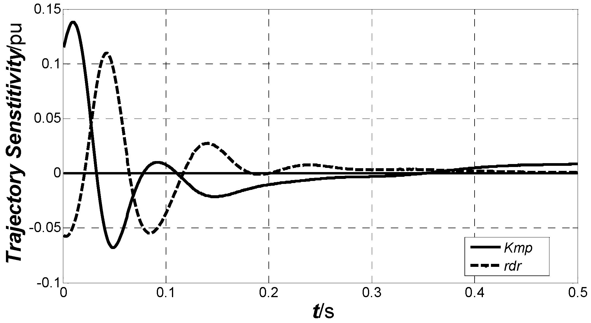
Trajectory sensitivity demonstrates the impact of the variation of the parameter on that of the output variable’s trajectory. If the trajectory sensitivity of a parameter is larger than that of the other parameters, the parameter plays a more important role on the dynamics of the output variable; in other words, the parameter can be estimated easily by using the dynamics of the output variable. In contrast, if the trajectory sensitivity of a parameter is very small, e.g., even close to zero, it is difficult to estimate the parameter using the dynamics of the output variable.

3.2. Trajectory Sensitivity Phase

If a couple of parameters have an unknown relationship between each other, they are dependent on each other and unidentifiable as well. However, these unidentifiable parameters can be identified using trajectory sensitivity analysis [29].
Assuming that the parameters θ i and θ i + 1 are coupling with each other, the output of the power system can be written as
y = f [ θ 1 , θ 2 , , φ ( θ i , θ i + 1 ) , , θ n ]
The sensitivities of the parameters θ i and θ i + 1 can be analyzed as [27]
{ y θ i = d y φ φ θ i y θ i + 1 = d y φ φ θ i + 1
Then
y θ i + 1 = d y θ i [ φ / θ i + 1 φ / θ i ]
It should be pointed out that y / θ i + 1 and y / θ i vary with time, while φ / θ i + 1 and φ / θ i are constant [29,30]. Hence, y / θ i + 1 and y / θ i reach zero at the same time. In other words, the trajectory sensitivities of these two couple unidentifiable parameters are either in phase or in reverse with each other. The trajectory sensitivity of these two parameters will pass zero at the same time. Oppositely, if the output variable curves of the two parameters do not pass zero at the same time approximately, they are independent and can be identified using the dynamics of output variables of the system [31].

4. Microgrid Parameter Estimation

4.1. Rotor Voltage Equivalence

Rotor voltage is an important operational variable in synchronous machine, and the parameters of the excitation system are estimated individually [32]. In the microgrid equivalent model, the excitation system is a virtual polymerization system, which maintains the terminal voltage. In [33], a synchronous machine with an excitation system is described by an asynchronous machine and a constant current load in load modeling. The dynamic of the synchronous machine is similar with the dynamic of the asynchronous machine and the constant current load. Hence, the rotor voltage of the equivalent microgrid model is replaced by a constant current load, which can be seen as a part of the equivalent static component in the modeling of microgrid.

4.2. Parameter Estimation Based on PSO

4.2.1. Review of Particle Swarm Optimization

Particle Swarm Optimization (PSO) is a heuristic optimization algorithm. It was first introduced by Kennedy and Eberhart, based on the observations of social behaviors of animals, such as bird flocking, fish schooling, and swarm theory [34]. This algorithm implements a global method that performs a search of parameters over a specified problem space. Like other evolutionary algorithms, PSO performs using a population of individuals that are updated iteratively. Swarm members communicate good position with each other and dynamically adjust their own position and velocity. Velocity adjustment is based upon the historical behaviors of the particles themselves as well as their neighbors. In each iteration, the velocity and position of each particle are updated according to the following equations.
v i ( k ) = w v i ( k 1 ) + c 1 r a n d 1 [ p b e s t i x i ( k 1 ) ] + c 2 r a n d 2 [ g b e s t x i ( k 1 ) ]
x i ( k ) = v i ( k ) + x i ( k 1 )
where x i is the position of the i th particle, v i is the velocity of the i -th particle, w is the inertia weight which decreases linearly determined by Equation (23), p b e s t i is the best position of the i -th particle, g b e s t is the global optimal position of the current swarm with the best objective value, c 1 and c 2 are acceleration constants, and r a n d 1 and r a n d 2 are two independent random numbers uniformly distributed over [0 1].
w = w min + w max w min k max × k
The algorithm achieves the optimal solution by two types of search memory, “cognitive” component and “social” component, which are shown as the second and third parts of Equation (21). The cognitive component makes the particle move toward its own best positions. The social component makes the particle toward the best position found by its neighbors, which means the collaborative behavior of particles.

4.2.2. Particle Swarm Optimization (PSO) with Chaos Neighborhood Searching

As optimization problem becomes more and more complex, the random characteristics of PSO will reduce the convergence velocity. In this paper, chaotic mutation theory is used to improve the global convergence velocity of the standard PSO. Chaos is a common phenomenon in non-linear systems that include infinite unstable period motions. Chaos-based neighborhood searching method with multiple different neighborhoods is designed and incorporated to enrich the searching behaviors, so as to avoid premature convergence [35]. In addition, an effective nonlinear adaptive inertia weight is employed to further enhance the exploitation ability after the chaos-based neighborhood searching.
Chaotic mapping is a discrete-time dynamical system, in which the chaotic sequences are considered as sources of random sequences, which can avoid getting stuck in a local optimum during the search process and overcomes the premature convergence phenomenon. Logistic mapping is a common chaos mapping, which is employed in the global optimal position neighborhood searching with the following steps.
(1)
Generating the initial variable u 0 j randomly based on the global optimal position of the particles.
(2)
Getting the chaotic sequences u 1 j using the logistic mapping u 1 j = 4 u 0 j ( 1 u 0 j ) .
(3)
Generating a local neighborhood mutation variable Δ x j : Δ x j = β + 2 β u 1 j , where β is the radius of the local neighborhood and is updated by Equation (24).
β = ( x j max x j min ) cos ( π ( t 1 ) 2 ( t max 1 ) )
where, t and t max are the round of the iteration and the maximal iteration times of the neighborhood searching, respectively. x j max and x j min are the upper and lower bounds of the variable x j , respectively.
(4)
Local neighborhood searching: A temporary global optimal position is defined as g b e s t = g b e s t + Δ X , where Δ X is the chaos mutation variables vector [ Δ x 1  Δ x j Δ x N ] and g b e s t = [ x g 1 x g N ] is the current global optimal position. Comparing g b e s t with g b e s t , the current global optimal position is updated by the larger one.

4.2.3. Improved Particle Swarm Optimization(IPSO) Based Parameter Estimation

IPSO algorithm is employed to search the optimal parameters of the microgrid equivalent model to achieve an optimal matching between the detailed model and the equivalent model of the microgrid. The steps of the IPSO-based microgrid equivalent model parameter estimation are shown in Figure 3.
Figure 3. Chart of Improved Particle Swarm Optimization (IPSO)-based parameter estimation.
Energies 08 12354 g003
(1) Initialization: From Section 2, there are 13 parameters, K m p , s 0 , r s , L s l , L a d , L a q , r d r , L d r l , r q r , L q r l , T j , p u and q u for the optimal parameter of the microgrid model. The initial particles may be generated randomly with a specified upper and lower bounds, X max and X min , respectively. The dimension of each particle is equal to the number of the parameters. Measured data include voltages ( u x + j u y ) and powers ( P + j Q ) of PCC.
The initial velocity of particles are generated randomly between the upper and lower bounds, v i , max and v i , min . Where the upper and lower bounds is defined by
v i , max = x i , max x i , min N v i , min = v i , max
where x i , max and x i , min are the upper and lower bounds of particles; and v i , max and v i , min are the maximum and minimum velocities of particles. N is the interval of dimension, which is normally chosen to be between 5 and 10.
(2) Evaluation: The Objective function is employed to evaluate each particle, and it is usually defined as the error between the measured power and the output power of the microgrid equivalent model as follows:
E ( θ ) = min k = 1 N { [ P ( k ) P M ( k , θ ) ] 2 + [ Q ( k ) Q M ( k , θ ) ] 2 }
where θ is the parameter vector of the equivalent model, P ( k ) and Q ( k ) are the measured power of sampling time k , and P M ( k , θ ) and Q M ( k , θ ) are the calculated power of the microgrid equivalent model. The aim of the objective function is that the output power of equivalent model can match the measured power.
(3) Updating movement velocities of the particles: Movement velocity updating is an important step in the process of evolution. The movement velocity of each particle is updated by Equation (21), and the velocity is limited in the upper and lower bounds as follows:
i f v i j ( t + 1 ) > v j , max t h e n    v i j ( t + 1 ) = v j , max i f v i j ( t + 1 ) < v j , min t h e n    v i j ( t + 1 ) = v j , min
(4) Updating positions of particles: The position of each particle is updated by Equation (22). The position of each particle is limited as follows
i f x i j ( t + 1 ) > x j , max t h e n    x i j ( t + 1 ) = x j , max i f x i j ( t + 1 ) < x j , min t h e n    x i j ( t + 1 ) = x j , min
(5) Chaos neighborhood searching: Following the steps described in the previous Section 4.2.2, the global optimal particle position is updated.
Firstly, an initial variable u 0 j is generated randomly, and the chaotic sequences u 1 j is generated by using the formula u 1 j = 4 u 0 j ( 1 u 0 j ) . Secondly, a local neighborhood mutation variable Δ x j is generated by using the formula Δ x j = β + 2 β u 1 j . Lastly, a new temporary global optimal position is generated which is the neighbor of the global optimal position. The fitness of the temporary global optimal position is compared with that of the current global optimal position, and the current global optimal position is replaced by the better one.
(6) Termination: The parameter estimation algorithm will be terminated if the iteration times exceeds the specified maximal iteration times or the fitness value of the global best is smaller than a given value.

5. Microgrid Equivalent Modeling and Discussion

5.1. Microgrid System

In this work, a microgrid system is built in DIgSILENT PowerFactory to test the effectiveness of the microgrid equivalent model and the feasibility of the modeling method. The structure of the microgrid is shown in Figure 4, and the detailed parameters and the operation mode can be found in [36]. The microgrid consists of wind generation, PV generation, micro-gas turbine, asynchronous induction motor and static load. The detailed parameters of microgrid are shown in Appendix A. The microgrid is radial and is connected to the distribution network through a 10 kv/20 kv transformer. The distribution network is a standard Benchmark medium voltage distribution network model in [37].
Figure 4. Microgrid system.
Energies 08 12354 g004
A single-phase short circuit is applied in the distribution network, and is cleared in 0.06 s. Using the dynamics of the exchange power between the microgrid and the distribution network, all the parameters of the equivalent model are estimated by the proposed PSO. The values of parameters used in PSO are depicted in Table 1. The algorithm has been implemented in C#.NET. The program runs on a 1.8 GHz, Intel Core2 Duo, with 2 GB RAM PC. The detail of the key parameters selected are: w max = 0.9 , w min = 0.4 , c 1 = c 2 = 2.0 , t max = 10 , k max = 500 . The bound of estimated parameters are shown in Appendix B. The estimated parameters are listed in Table 1, and the dynamics of the output power of the detailed model and the equivalent model are illustrated in Figure 5. It can be seen that the dynamics of the output power of the equivalent model is approximate to that of the detailed model.
Figure 5. (a) The active power dynamics of the detailed model and the equivalent model of the Microgrid; (b) The reactive power dynamics of the detailed model and the equivalent model of the Microgrid.
Energies 08 12354 g005
Table 1. A group of feasible parameters for the equivalent model.
ParameterKmps0rsLslLadLaprdr
Value−8.70−0.2060.0310.3400.8483.140.00023
Parameter L d r l r q r L q r l T j p u q u Error
Value2.180.1710.7569.667.060.7312.401
The evolution of function objective is presented along the iterations in order to observe the behavior of improved PSO, and to verify if the PSO works as expected. Figure 6 shows the evolution of function objective along with the iterations. It can be seen from the graph that the objective function has converged to a constant value of 2.401 after 57 iterations. It is quite apparent that the improved PSO has the faster convergence than the standard PSO algorithm. Moreover, the proposed IPSO and standard PSO achieved in the same machine converged their corresponding optimal solutions in 25.3 s and 37.5 s, respectively.
Figure 6. Convergence of the improved particle swarm optimization (IPSO) and PSO Algorithms.
Energies 08 12354 g006

5.2. Parameter Sensitivity Analysis and Error Analysis

The number of parameters to be estimated has a significant impact on the accuracy of the parameter estimation. If only the key parameters are estimated, the convergence of the PSO can be improved and the probability finding the true value of the parameters will be higher.
The sensitivities of the equivalent microgrid model parameters, θ = [ K m p , s 0 , r s , L s l , L a d , L a q , r d r , L d r l , r q r , L q r l , T j , p u , q u ] , with respect to the trajectory of the apparent power S , are calculated. S is defined as:
S = P M 2 + Q M 2
where P M and Q M are the calculated active and reactive power based on the dynamic equivalent model of equal Equation (26).
The average trajectory sensitivities of the parameters are listed in Table 2, and the dynamics of the trajectory sensitivities are shown in Figure 7. It can be seen in Table 2 that the parameters K m p , s 0 , L a d , L a q , r d r , L d r l , L q r l and p u have more significant impacts on the trajectory than the other parameters. Figure 7 shows that the phases of the sensitivity of K m p , is almost reverse to that of r d r , which means that K m p and r d r are related with each other and are unidentifiable by using the dynamics of S . As a result, only the seven parameters, i.e., K m p , s 0 , L a d , L a q , L d r l , L q r l and p u , are included in the further steps of the parameter estimation, while the other parameters are set as default values.
Table 2. Parameter sensitivity absolute value.
ParameterKmps0rsLslLadLaprdr
Sensitivity0.01600.03520.00160.00400.13670.03770.0149
Parameter L d r l r q r L q r l T j p u q u
Sensitivity0.15430.000430.05830.00150.01200.0011
Figure 7. The trajectory sensitivity of parameter K m p and r d r .
Energies 08 12354 g007

5.3. Key Parameters Estimation and Error Analysis

By using the dynamics of the output power of the detailed model of microgrid, the key parameters are estimated and listed in Table 3. The dynamics of the output active power and reactive power are also illustrated in Figure 8a,b, respectively. As can be seen in Figure 8, the amplified windows show the differences of the two estimated method, and it is clear that the error between the dynamics of the output power of the equivalent model and the detailed model is smaller than that when all the parameters are estimated simultaneously, as shown in Table 1.
The simulation results reveal that the proposed dynamic equivalent model is accurate enough to describe the dynamic characteristics of the microgrid detailed model quickly during the simulation period. The equivalent model can track the fluctuation of active power and reactive power quickly and flexibly, especially in the moment of fault cutting. The estimated results of parameters are suitable according to the electrical parameter standards.
Figure 8. (a) The active power dynamics of microgrid; (b) The reactive power dynamics of microgrid.
Energies 08 12354 g008
Table 3. Parameter estimated value.
ParameterKmps0LadLapLdrlLqrlpuError
Value−8.637−0.21610.80423.4172.1200.70087.0392.389
Because the proposed model is an equivalent model in electromechanical transient, the stator transient is neglected during the process of equivalent modeling, which will bring some error both in parameters and dynamic of the microgrid. In Figure 8a, it can be seen that at the time of the single-phase short fault occurs and cleared, the error between equivalent model and the detailed model is larger than other time relatively. At this moment, the active power of equivalent model cannot track the dynamic of microgrid completely. The components of microgrid are various and the dynamic of the output power of microgrid contains different components. In order to improve the representational capacity of the equivalent model, some elements are ignored, such as the stator transient of wind turbine and micro-gas turbine, the transient of PV inverter.

5.4. Comparing to Other Models

The proposed microgrid equivalent model is also compared with the equivalent machine component model and black-box model. The equivalent microgrid model contains two parts: equivalent machine component and equivalent static component. The equivalent machine component is used to describe the rotor characteristics of electrical equipment, and the equivalent static component is used to describe the characteristics of steady state of microgrid.
The equivalent machine model is compared with the comprehensive model in this paper. This means that the values of the parameters are K m p = 1 , p u = 0 and q u = 0 . Figure 9 shows the dynamics between different models of the microgrid. It can be seen that the error between the proposed equivalent microgrid model and detailed model is smaller than that of the equivalent machine model and detailed model. As can be seen in Figure 9b, the output reactive power of the proposed equivalent microgrid model can track the detailed model more accurately than that of the equivalent machine component model during the fault. It means that the equivalent static component is important in the proposed equivalent microgrid model. The equivalent static component can describe the dynamic characteristics of static component in the microgrid, such as: photovoltaic system, static load, and other static equipment.
Figure 9. (a) Dynamics of Active Power of different models; (b) Dynamics of Reactive Power of different models.
Energies 08 12354 g009
The proposed microgrid equivalent model is based on the physics characteristics of the electrical components in microgrid, and can describe the electrical physical characteristics of microgrid components. Non-mechanism model is also used in the dynamic equivalent of power system. In the equivalent modeling of microgrid, a dynamic equivalent black-box model based on prony analysis is presented in [38], the proposed equivalent model is compared with the black-box equivalent model. Figure 10 shows the comparison the proposed model and the black-box model; it can be seen that the two models are in good agreement with the detailed model, and the proposed model is more accurate.
Figure 10. (a) Dynamics of Active Power of different models; (b) Dynamics of Reactive Power of different models.
Energies 08 12354 g010

5.5. Parameters Estimation under Different Operational Conditions

The operational condition of the microgrid changes with the fluctuation of the distributed generation output power and the variation of loads, which leads to the power exchange between the microgrid and the distribution network changes accordingly. Therefore, the parameters of the microgrid equivalent model should be adjusted to adapt the changes of the microgrid operational condition. Three different typical operational conditions are studied in the paper, the detailed operational parameters are shown in Table 4 and the parameters estimated results are shown in Table 5.
Table 4. Describe of operational conditions.
Operational ConditionDescription
Condition AThe output power of gas turbine reduces 40 percent with the output active power is 3 MW.
Condition BThe output power of gas turbine reduces 40 percent with the output active power is 3 MW, 40 percent of Static Load 2, which is 2 MW active power and 0.4 Mvar reactive power, is removed.
Condition CThe output power of gas turbine reduces 40 percent with the active power is 3 MW. The output active power of Wind Generation reduces a half, which become 0.75 MW. PV is removed. 40 percent of Static Load 1, which is 0.4 MW and 0.2 Mvar, is removed.
As can be seen in Table 5, the equivalent machine component outputs active power as a generator with K m p < 0 and s 0 < 0 , while the microgrid absorbs power from the distribution network in condition A. This means that the consume power of equivalent static component comes from distribution network and equivalent machine component. In conditions B and C, the equivalent machine component absorbs power as an asynchronous induction motor with K m p > 0 and s 0 > 0 , while the microgrid absorbs power from the distribution network.
Table 5. Parameter value of different operational conditions.
ParameterKmps0rsLslLadLaqrdrLdrlrqrLqrlTjpuqu
Condition A−4.69−0.170.05900.361.942.500.00033.040.25602.245.624.870.94
Condition B1.640.070.06100.104.057.540.11861.490.00244.005.188.950.61
Condition C0.990.120.04920.313.704.760.14500.650.00574.006.553.580.70
In condition A, with the power reduction of gas turbine, microgrid may absorb more power from distribution network. Figure 11 shows microgrid response to the single-phase short fault in distribution network. The exchange power between microgrid and distribution network fluctuates violently, but the results show the great agreement between proposed equivalent model and the detailed model, and the reactive power of equivalent model can track the detailed model with a small time delay.
Figure 12 and Figure 13 show the response of dynamic equivalent model during the fault of condition B and condition C. The microgrid construction of condition B and C is similar, and it can be seen that the dynamics of the equivalent model coincide with that of the detailed model well. Especially during the fault, the errors between equivalent model and detailed model are very small.
Furthermore, Table 5 shows the stability of estimated parameters of equivalent model in different microgrid operational conditions, and the equivalent model can descript the dynamic of microgrid under different operational condition, which means that the equivalent model is robust.
Figure 11. (a) The active power dynamics of the detailed model and the equivalent model under condition A; (b) The reactive power dynamics of the detailed model and the equivalent model under condition A.
Energies 08 12354 g011
Figure 12. The active power dynamics of the detailed model and the equivalent model under condition B.
Energies 08 12354 g012
Figure 13. The active power dynamics of the detailed model and the equivalent model under condition C.
Energies 08 12354 g013

6. Conclusions

The equivalent model of the microgrid, based on electrical equipment physical characteristics, is proposed in this paper. The equivalent model consists of an equivalent machine component and an equivalent static component. Equivalent machine component is used to describe the dynamic of rotor machine characteristics and equivalent static component is used to describe the comprehensive characteristics of static component. In order to clear up the importance of each parameter toward the dynamics of the model, time-domain sensitivity of the parameters of the equivalent model with respect to the output power of the microgrid has been analyzed. The key parameters with important impact on the dynamics of the equivalent model have been detected. An improved particle with variable neighborhood searching is proposed where the radius of neighborhood is changed based on chaos iteration. The improved particle swarm optimization (IPSO) algorithm is used for parameters estimation, which improves the accuracy of the parameter estimation. The simulation results of microgrid under different operation conditions show that the simplified equivalent model is in good agreement with the detailed model under fault. The proposed model can be combined with other electrical component model in the power system simulation platform. With the proposed equivalent model, we can simplify the detailed model of microgrid obviously, and improved the simulation speed of power system.

Acknowledgments

This paper was sponsored by the Open Fund of Jiangsu Key Laboratory of Power Transmission & Distribution Equipment Technology (2011JSSPD11) and Science and technology project of Changzhou (CE20130043). The authors are also grateful to College of the Internet of Things Engineering and Jiangsu Key Laboratory of Power Transmission & Distribution Equipment Technology, at Hohai University, China.

Author Contributions

Changchun Cai presented the equivalent model of microgrid and designed the experiments, performed the experiments, written the article. Bing Jiang and Lihua Deng analyzed the data and modified the article.

Conflicts of Interest

The authors declare no conflicts of interest.

Appendix A. Detail Data of Microgrid

Table A1. Wind Generator Parameters.
UN/kVSN/MVAcosφRs/puXs/puRr/puXr/puXμ/puTj/s
0.962.40.87560.01000.10000.01000.10003.00001.188
Table A2. Gas Turbine Parameters.
UN/kVSN/MVArs/puXd/puXq/puX′d/puX″d/puX′q/puX″q/puT′d0/sT′q0/sT″d0/sT″q0/s
0.44801.51.50.2560.070.30.070.017100.01250.0057
Table A3. Rotor Load Parameters.
LoadUN/kVPN/kVAsrs/puXs/puRr/puXr/puXμ/puTj/s
Load 10.4150315.0 × 20.0275600.02000.03470.20222.3900.6230
Load 20.4150315.0 × 50.0275600.02000.03470.20222.3900.6230
Table A4. Static Load Parameters.
LoadP + Q
Load 11 MW + 0.5 MVar
Load 25 MW + 1 MVar

Appendix B. Parameters Used in the PSO

Table B1. The bounds of the parameters.
xmin−10−0.3000000000−1−1
xmax100.30.20.55100.250.5510105

References

  1. Lasseter, B. Microgrids. In Proceeding of the Power Engineering Society Winter Meeting, New York, NY, USA, 28 January–1 February 2001; pp. 146–149.
  2. Delghavi, M.B.; Yazdani, A. Islanded-Mode control of electronically coupled distributed-resource units under unbalanced and nonlinear load conditions. IEEE Trans. Power Deliv. 2011, 26, 661–673. [Google Scholar] [CrossRef]
  3. Zhang, M.R.; Chen, J. The Energy Management and Optimized Operation of Electric Vehicles Based on Microgrid. IEEE Trans. Power Deliv. 2014, 29, 1427–1435. [Google Scholar] [CrossRef]
  4. Xiong, L.; Peng, W.; Chiang, L.P. A hybrid AC/DC microgrid and its coordination control. IEEE Trans. Smart Grid 2011, 2, 278–286. [Google Scholar] [CrossRef]
  5. Logenthiran, T.; Srinivasan, D.; Khambadkone, A.M.; Aung, H.N. Multiagent system for real-time operation of a Microgrid in real-time digital simulator. IEEE Trans. Smart Grid 2012, 3, 925–933. [Google Scholar] [CrossRef]
  6. Yang, B.; Li, W.H.; Zhao, Y.; He, X.N. Design and analysis of a Grid-Connected photovoltaic power system. IEEE Trans. Power Electron. 2010, 25, 992–1000. [Google Scholar] [CrossRef]
  7. Piazza, M.C.D.; Luna, M.; Vitale, G. Dynamic PV model parameter identification by least-squares regression. IEEE J. Photovolt. 2013, 3, 799–806. [Google Scholar] [CrossRef]
  8. Keyhani, A. Modeling of photovoltaic microgrids for bulk power grid studies. In Proceeding of the Power and Energy Society General Meeting, Detroit, MI, USA, 24–28 July 2011; pp. 1–6.
  9. Castro, R.M.G.; de Jesus, J.M.F. A wind park reduced-order model using singular perturbations theory. IEEE Trans. Energy Convers. 1996, 11, 735–741. [Google Scholar] [CrossRef]
  10. Conroy, J.; Watson, R. Aggregate modelling of wind farms containing full-converter wind turbine generators with permanent magnet synchronous machines: Transient stability studies. IET Renew. Power Gener. 2009, 3, 39–52. [Google Scholar] [CrossRef]
  11. Wang, H.H.; Tang, Y.; Hou, J.X.; Zhou, J.F.; Liang, S.; Su, F. Equivalent method of integrated power generation system of wind, photovoltaic and energy storage in power flow calculation and transient simulation. Proc. CSEE 2011, 32, 1–8. [Google Scholar]
  12. Rubio, J.J.; Figueroa, M.; Pacheco, J.; Jimenez-Lizarraga, M. Observer design based in the mathematical model of a wind turbine. Int. J. Innov. Comput. Inf. Control 2011, 7, 6711–6725. [Google Scholar]
  13. Ali, M.; Ilie, I.S.; Milanovic, J.V.; Chicco, G. Wind farm model aggregating using probabilistic clustering. IEEE Trans. Power Syst. 2013, 28, 309–316. [Google Scholar] [CrossRef]
  14. Zha, X.M.; Zhang, Y.; Cheng, Y.; Fan, Y.P. New method of extended coherency for Microgrid based on homology in differential geometry. Trans. China Electrotech. Soc. 2012, 27, 24–31. [Google Scholar]
  15. Ju, P.; Handschin, E.; Karlsson, D. Nonlinear dynamic load modelling model and parameter estimation. IEEE Trans. Power Syst. 1996, 11, 1689–1697. [Google Scholar] [CrossRef]
  16. Abido, M.A. Multi-objective evolutionary algorithms for electric power dispatch problem. IEEE Trans. Evolut. Comput. 2006, 10, 315–329. [Google Scholar] [CrossRef]
  17. Wang, S.K.; Chiou, J.P.; Liu, C.W. Parameters tuning of power system stabilizers using improved ant direction hybrid differential evolution. Int. J. Electr. Power Energy Syst. 2009, 31, 34–42. [Google Scholar] [CrossRef]
  18. Fogel, D.B. Evolutionary Computation: Toward a New Philosophy of Machine Intelligence, 2nd ed.; IEEE Press: New York, NY, USA, 2000. [Google Scholar]
  19. Lu, Z.; Ji, T.Y.; Tang, W.H.; Wu, Q.H. Optimal harmonic estimation using a particle swarm optimizer. IEEE Trans. Power Deliv. 2008, 23, 1166–1174. [Google Scholar] [CrossRef]
  20. Iashif, K.; Salam, Z.; Amjad, M.; Mekhilef, S. An improved particle swarm optimization (PSO)-Based MPPT for PV with reduced steady-state oscillation. IEEE Trans. Power Electron. 2012, 27, 3627–3638. [Google Scholar] [CrossRef]
  21. Ye, M.Y.; Wang, X.D.; Xu, Y.S. Parameter identification for proton exchange membrane fuel cell model using particle swarm optimization. Hydrog. Energy 2009, 34, 981–989. [Google Scholar] [CrossRef]
  22. Huynh, D.C.; Dunnigan, M.W. Parameter estimation of an induction machine using advanced particle swarm optimization algorithms. IET Electr. Power Appl. 2010, 49, 748–760. [Google Scholar] [CrossRef]
  23. Zeng, N.Y.; Wang, Z.D.; Li, Y.R.; Du, M.; Liu, X.H. A hybrid EKF and Switching PSO algorithm for Joint State and Parameter Estimation of Lateral Dlow Immunoassay Models. IEEE Trans. Comput. Biol. Bioinf. 2012, 9, 321–329. [Google Scholar] [CrossRef] [PubMed]
  24. Panigrahi, T.; Panda, G.; Mulgrew, B. Distributed bearing estimation techinque using diffusion particle swarm optimation algorithm. IET Wirel. Sens. Syst. 2012, 2, 385–393. [Google Scholar] [CrossRef]
  25. Kanchev, H.; Lu, D.; Colas, F.; Lazarov, V.; Francois, B. Energy management and operational planning of a Microgrid with a PV-Based active generator for smart grid applications. IEEE Trans. Ind. Electron. 2011, 58, 4583–4592. [Google Scholar] [CrossRef] [Green Version]
  26. IEEE. Task Force on Load Representation for Dynamic Performance Load representation for dynamic performance analysis. IEEE Trans. Power Syst. 1993, 8, 472–482. [Google Scholar] [CrossRef]
  27. Wu, F.; Zhang, X.P.; Godfrey, K.; Ju, P. Small signal stability analysis and optimal control of a wind turbine with doubly fed induction generator. IET Gener. Transm. Distrib. 2007, 1, 751–760. [Google Scholar] [CrossRef]
  28. Kunder, P. Power System Stability and Control, 1st ed.; China Electric Press: Beijing, China, 2001. [Google Scholar]
  29. Ju, P.; Qin, C.; Wu, F.; Xie, H.L.; Ning, Y. Load modeling for wide area power system. Int. J. Electr. Power Energy Syst. 2011, 33, 909–917. [Google Scholar] [CrossRef]
  30. Rubio, J.J. Modified optimal control with a back propagation network for robotic arms. IET Control Theory Appl. 2012, 6, 2216–2225. [Google Scholar] [CrossRef]
  31. Pérez-Cruz, J.H.; Rubio, J.J.; Ruiz-Velázquez, E.; Solís-Perales, G. Tracking control based on recurrent neural networks for nonlinear systems with multiple inputs and unknown dead-zone. Abstr. Appl. Anal. 2012, 2012. [Google Scholar] [CrossRef]
  32. Puma, J.Q.; Colome, D.G. Parameters identification of excitation system models using genetic algorithms. IET Gener. Transm. Distrib. 2008, 2, 456–467. [Google Scholar] [CrossRef]
  33. Wang, J.L. Study on Special Load Modeling in Power System. Ph.D. Thesis, North China Electric Power University, Beijing, China, 2010. [Google Scholar]
  34. Giaquinto, A.; Fornarelli, G. PSO-Based cloning template design for CNN associative memories. IEEE Trans. Neural Netw. 2009, 20, 1837–1841. [Google Scholar] [CrossRef] [PubMed]
  35. Jiang, C.W.; Bompard, E. A hybrid method of chaotic particle swarm optimization and linear interior for reactive power optimization. Math. Comput. Simul. 2005, 68, 57–65. [Google Scholar] [CrossRef]
  36. Cao, X.Q.; Ju, P.; Cai, C.C. Simulative analysis equivalent reduction for Microgrid. Electr. Power Autom. Equiv. 2011, 31, 94–98. [Google Scholar]
  37. Rudion, K.; Styczynski, Z.A.; Hatziargyriou, N.; Papathanassiou, S. Development of benchmarks for low and medium voltage distribution networks with high penetration of dispersed generation. In Proceedings of the 3rd International Symposium on Modern Electric Power Systems, Wroclaw, Poland, 6–8 September 2006.
  38. Papadopoulos, P.N.; Papadopoulos, T.A.; Crolla, P.; Roscoe, A.J.; Papagiannis, G.K.; Burt, G.M. Black-box dynamic equivalent model for microgrid using measurement data. IET Gener. Transm. Distrib. 2014, 8, 851–861. [Google Scholar] [CrossRef] [Green Version]

