In this article, a brief overview of the UCG reactor sub-model of forward gasification is particularly discussed due to its direct impacts on coal resource recovery, cavity growth, energy efficiency and, consequently, economic feasibility.
Since there are a number of mathematical/numerical models in the literature, it is most instructive to indicate the significant features and limitations of these models. Most of the earlier models were one-dimensional (1D); however, with the advancement of computational power, two-dimensional (2D) and even a few three-dimensional (3D) models were developed. In the following section, the various modeling approaches are discussed.
2.1. Packed Bed Models
The earliest models of UCG in literature include models that describe the process as a packed bed reactor. The consideration of the “
in-situ” coal seam as a packed bed primarily originated from the concept of Higgins [
41] considering the creation of a permeable zone between two boreholes either by reverse combustion linking (RCL) or by fracturing the coal seam using pressurized air or chemical explosives [
42,
43]. The resultant coal seam resembles a packed bed where coal particles are filled in the reactor. This concept is similar to the major Soviet approach to seam preparation where they included extensive drying of the seam and reverse combustion to obtain a region of enhanced permeability between the boreholes [
44]. On the other hand, according to Gunn and Whitman [
45], the coal seam consists of lignite or subbituminous coal can be gasified without establishing any linkage path due to their high permeability, also known as the percolation or filtration method which more closely resembles the operation of a packed bed chemical reactor. The packed bed model assumes that coal gasification occurs in highly permeable porous media with a stationary coal bed which is consumed over time [
46].
Table 4 and
Table 5 represent a glimpse of a list of packed bed models discussed here with their essential features and reaction rate control mechanisms of the main reactions in the gasification process, respectively.
Initially, around 1976, several 1D transient packed bed models [
42,
47,
48] with the finite-difference approach were developed in parallel, supported by the Lawrence Livermore National Laboratory (LLNL) program. However, there is no basic difference between the models developed by Thorsness
et al. [
48] and Thorsness and Rozsa [
42]. Thorsness and Rozsa [
42] provided a detailed description of the lab-scale gasification experiment whereas Thorsness
et al. [
48] provided a detailed description of the development of the physical and chemical model where they made many simplifying physical and chemical assumptions, based on experimental and theoretical comparisons and correlations, which include:
- -
the gas permeability.
- -
the effective thermal conductivity.
- -
the interphase heat-transfer coefficient.
- -
the chemical reaction rates.
- -
the various thermodynamic properties of each species, and.
- -
the stoichiometric coefficients.
In their model, they neglected tar condensation and plugging, gas losses to surroundings, water intrusion from surroundings, heat losses, and coal bed movement due to shrinking or swelling during drying and pyrolysis in order to avoid complexity.
Winslow [
47] also followed their work, except using a different numerical solution scheme. Thorsness
et al. [
48] considered all the main reactions for gasification (reaction 1 to reaction 10); however, for homogeneous reactions, only the water-gas shift reaction was considered by Winslow [
47]. Although, for convenience, most of the researchers represent char as a molecule containing one carbon, they considered the chemical formula of char and dry coal as CH
a1O
b1 and CH
a2O
b2, respectively, where the composition parameters a1, b1, a2, b2 depend on the type of coal (usually obtained from the ultimate analysis). Beside the moisture content for drying, they also considered mobile condensed water which undergoes evaporation and condensation upon the removal of heating. However, for the simplicity of the calculation, they assumed a fixed velocity of mobile water. Their model considered fitted kinetic models for pyrolysis data developed by Campbell [
49]. The controlling mechanisms of reaction rates that they considered are listed in
Table 5. Eight gas species (N
2, O
2, H
2O, H
2, CH
4, CO, CO
2, tar) and five solid/condensed species (coal, char, mobile liquid water, fixed liquid water, and ash) were considered, upon which the balances were written. The reaction rates of the heterogeneous reactions (char-gas reactions) were considered to be influenced by three mechanisms: mass-transport limitation from the bulk gas to the solid surface, mass-transport limitations in any internal particle porosity, and kinetic limitations at the solid surface. This reaction mechanism was also considered for the water-gas shift reaction due to the influence of a catalyst that might be present in the coal bed. Because of the high reactivity of char as compared to pure carbon, the mass transfer limitation was considered important. However, in their model, one effective chemical rate expression (
Rc) was assumed in order to account for the internal transport and surface kinetics. As a result, the total rate (
RT) was considered as a kinetic internal-diffusion rate and expressed as follows:
where
Rc is linearly dependant on the mole fraction of the limiting reactant (
yl) in the bulk phase and the parameter
Rm is the mass transfer rate of a limiting reaction defined by:
where
ky is the mass transfer coefficient.
In their models, the fluid flow was described by the Darcy equation, in which permeability was set to change with the extent of the reactions. From the experimental data of drying and pyrolysis of subbituminous Wyodak coal, they formulated a functional relationship relating permeability to porosity that was used later by a number of researchers [
12,
47,
50] who developed their model using subbituminous coal. The relationship is as follows:
where
αo is the initial permeability,
φo is initial porosity of coal, and
φlim is the upper limit of porosity above which the permeability was assumed to be constant. Based on the experiment, the calculated value of the parameter σ was approximately 12. In their report, they considered
φlim = 0.25 so that the particle size decreases with increasing porosity (
φ < 0.25). As a result, the permeability was assumed to reach a constant value for porosity larger than 0.25.
Thorsness
et al. [
48] incorporated a quasi-steady approximation for changes associated with the gas phase that allowed them to use ordinary differential equations for gas phase mass and energy balances. The governing equations were as follows:
Mass balance:
where G is the number of gas species.
It is noted that gas phase diffusion, which had been considered an important factor in the channel and coal slab model development, was neglected.
where K is the number of solid/condensed species.
Momentum balance:
The momentum balance gas phase was replaced by Darcy’s law:
The use of Darcy’s law and some theoretical correlations they employed in their model indicate an implicit assumption of the laminar flow process.
On the other hand, Winslow [
47] did not approximate any stationary phase for the basic conservation equation, although he followed the physical and chemical model of Thorsness
et al. [
48]. The following governing equations for mass and energy balance for both the gas and solid phases were used by Winslow [
47]:
where G is the number of the gas species. Gas diffusion was neglected.
where K is the number of solid/condensed species.
Using Darcy’s law, the gas bulk velocity is given by:
Table 4.
Some essential features of reported packed bed models.
Table 4.
Some essential features of reported packed bed models.
| Researchers | Dimension and Time Dependence | Heat Transfer | Mass Diffusion | Fluid Flow | Thermo Mechanical Failure | Water Influx | Heat Loss |
|---|
| Conduction | Convection | Radiation |
|---|
| Winslow [47] | 1D & T | √ | √ | | | D | | | |
| Thorsness et al. [48] | | | | | | | | | |
| Thorsness and Rozsa [42] | 1D & T | √ | √ | | | D | | | |
| Khadse et al. [46] | 1D & PS | √ | √ | | | D | | | |
| Uppal et al. [43] | 1D & PS | √ | √ | | | D | | | |
| Thorsness and Kang [51] | 1D & T | √ | √ | | √ | D | √ | | |
| Gunn and Whitman [45] | 1D & PS | √ | | | √ | | | √ | |
| Abdel-Hadi and Hsu [8] | 1D & T | √ | √ | | √ | | | | |
Table 5.
Reaction rate control mechanisms of the main reactions in the gasification process.
Table 5.
Reaction rate control mechanisms of the main reactions in the gasification process.
| Researchers | Drying | Pyrolysis | Char Reaction | Water-Gas Shift Reaction | Gas Phase Reaction |
|---|
| C + O2 → CO2 | C + CO2 → 2CO | C + H2O → CO + H2 | C + 2H2 → CH4 | CO + H2O ↔ CO2+ H2 | CO + 0.5O2 → CO2 | H2 + 0.5O2 → H2O | CH4 + 2O2 → CO2 + 2H2O |
|---|
| Winslow [47] | D | P | K | K | K | K | K | | | |
| Thorsness et al. [48] | D | P | K | K | K | K | K | I | I | I |
| Thorsness and Rozsa [42] | D | P | K | K | K | K | K | I | I | I |
| Khadse et al. [46] | | P | K | K | K | K | K | | | |
| Uppal et al. [43] | | P | K | K | K | K | K | I | I | I |
| Thorsness and Kang [51] | | | K | K | K | K | K | I | I | I |
| Gunn and Whitman [45] | | EC | P | | P | | | | | |
| Abdel-Hadi and Hsu [8] | D | P | P | P | P | P | E | | | |
The primary objective of their preliminary works was to predict and correlate reaction and thermal-front propagation rates and product-gas composition as a function of coal bed properties and process operating conditions, as well as the secondary objective of testing the correctness of the physical and chemical model they developed. Despite the simplifying assumptions as shown in
Table 6, their results were generally in accordance with steady-state laboratory measurements (
Table 7) Experimental run 5 was carried out using back heating in order to eliminate radial heat losses. As a result, model calculations with the assumption of no heat loss were closer to the data of experimental run 5. Although the lab-scale experiment did not represent the field-scale system as the porosity (50%) and the permeability (150 D) were too high and the particle diameter (1 cm) was too small, the agreement between the model calculations and the lab experiments indicates that the simple physical and chemical models of Thorsness
et al. [
48] are useful to some extent in the design of the gasification process.
Table 6.
Input parameters used for model calculation and experimental runs from a 1.6 m reactor.
Table 6.
Input parameters used for model calculation and experimental runs from a 1.6 m reactor.
| Input Parameters | Calculated (Thorsness and Rozsa [42], Thorsness et al. [48]) | Calculated
(Winslow [47]) | Reactor experiments (Thorsness and Rozsa [42], Thorsness et al. [48]) |
|---|
| | | | Run 4 (no backheating) | Run 5 (with backheating) |
| Coal Dimension | L = 150 cm,
D =15 cm | L = 150 cm,
D =15 cm | L = 150 cm,
D =15 cm | L = 150 cm,
D = 15 cm |
| Initial Porosity | 50% | 44.4% | 50% | 50% |
| Initial Permeability | 150 Darcy | | 150 Darcy | 150 Darcy |
| Coal Particle Size | 1 cm | 1 cm | 1 cm | 1 cm |
| Injected Gas Flow Rate | 2 × 10⁻⁴ gmole/cm2·s | 2.1 × 10⁻⁴ gmole/cm2·s | 2 × 10⁻⁴ gmole/cm2·s | 2 × 10⁻⁴ gmole/cm2·s |
| Initial Feed Temperature | 450 K | 450 K | 450 K | 450 K |
| Pressure | 4.8 Atm | 4.8 Atm | 4.8 Atm | 4.8 Atm |
| Injected Gas Composition |
| O2 | 14.1% | 13.4% | 13.4% | 13.4% |
| N2 | 24.0% | 22.0% | 22.0% | 22.0% |
| H2O | 83.5% | 84.4% | 84.4% | 84.4% |
| Steam/O2 Ratio | 6 | 6 | 6 | 6 |
Table 7.
Steady-state temperature and major constituents of outlet gas composition.
Table 7.
Steady-state temperature and major constituents of outlet gas composition.
| Parameters | Calculated (Thorsness and Rozsa [42], Thorsness et al. [48]) | Calculated (Winslow [47]) | Measured (average over run) (Thorsness and Rozsa [42], Thorsness et al. [48]) |
|---|
| | | | Run 4 (no back heating) | Run 5 (with back heating) |
| Peak Temperature (K) | | 1250 | | 1200 |
| Speed of burn front | 18 cm/h | 18 cm/h | | 18 cm/h |
| Product Gas Composition (dry basis) |
| H2 | 43.2% | 43.8% | 44.9% | 44.6% |
| CH4 | 6.6% | 4.0% | 6.4% | 6.9% |
| CO | 22.0% | 22.0% | 16.5% | 19.0% |
| CO2 | 28.2% | 30.2% | 33.2% | 29.5% |
Beside the model validation with experimental data, they also illustrated various features of their simulations with time or spatial variations and compared them with the experimental results where possible. The solid and gas temperature distribution along the length in their system at different times indicated the propagation of the reaction and drying/pyrolysis fronts at different speeds (see
Figure 3).
Figure 3.
Calculated gas and solid temperature at three different times for the 1.5 m reactor simulation [
48].
Figure 3.
Calculated gas and solid temperature at three different times for the 1.5 m reactor simulation [
48].
The different fronts that were growing at different speeds associated with the movement of the gasification process were also recognized from the plot of the reaction rate as a function of bed length (
Figure 4). Those were the coal drying front, then the coal pyrolysis front, followed by the char reaction front considering moving upstream from the outlet. The double-peak of the water-gas shift reaction was due to the changes in equilibrium limits because of changes in temperature (
Figure 4). The gas concentration along the bed length showed that the inlet gas composition remained unreacted until the reaction front (
Figure 5). However, after an initial rapid change followed by a more gradual one, a sharp change in gas concentration was observed due to the drying-pyrolysis front. Winslow [
47] also observed the same trend.
Figure 4.
Distribution of principal reaction rates at
t = 1 h 13 min [
47].
Figure 4.
Distribution of principal reaction rates at
t = 1 h 13 min [
47].
Figure 5.
Calculated gas phase concentration at time = 1.4 × 10
4 s for the 1.5 m reactor simulation [
48].
Figure 5.
Calculated gas phase concentration at time = 1.4 × 10
4 s for the 1.5 m reactor simulation [
48].
A comparison of the position of the calculated reaction and drying front with experimental data showed that the results were in good agreement with the reaction front; however, the predicted drying front movement rate was found higher than the experimental findings (see
Figure 6). According to them, the latter observation was due to some uncertainty of the product gas mix and the heat losses occurring during the experiment at the drying zone.
Figure 6.
Comparison of calculated and experimental reaction and drying front movements [
48].
Figure 6.
Comparison of calculated and experimental reaction and drying front movements [
48].
Thorsness
et al. [
48] extended their works by reporting very limited parametric study. For example, with increasing oxygen concentration in the feed gas (holding a constant gas flow rate), they observed an increased gas/solid temperature and the drying rate of the reaction front moved linearly with oxygen concentration. An increased ratio of CO to CO
2 resulting from the increased temperature generation in the system was also detected. With the increase of total dry gas production, a consistent CO/CO
2 ratio was also noticed with the higher oxygen feed. However, for energy recovery per mole of O
2, they indicated an optimum value of oxygen consumption at a mole fraction of approximately 0.2 (see
Figure 7). This observation is actually set a limit for the steam-to-oxygen ratio at a value of 4 for maximum energy recovery.
Figure 7.
Calculated energy recovery for three levels of oxygen feed concentration [
48].
Figure 7.
Calculated energy recovery for three levels of oxygen feed concentration [
48].
There was an attempt by Thorsness
et al. [
48] to simulate a field-scale system with length equal to 15 m, porosity equal to 0.05, permeability equal to 20 D, outlet pressure equal to 1 atm, and particle diameter equal to 20 cm. However, they could not validate the changes of the process variable except the developing temperature profile that was similar to their lab-scale simulation.
Although they showed time and distance changes in the process variable in the principal direction of gas flow, they did not conduct a detailed sensitivity analysis to investigate the effect of coal particle diameter, porosity, permeability, injection gas flow rate, and other parameters in their model despite the fact that the basis of the model formulation was a 1 cm particle diameter. This imposes the use of their model for specific conditions. The applicability of their model to field conditions where the particle diameter is approximately equal to 20 cm is limited because of the lack of sensitivity of the results to particle size and the validation of field trials. The particle size is particularly important because, in their physical and chemical model, the char reaction rates and other transport coefficients such as heat transfer and mass transfer coefficients are directly or indirectly related to the particle sizes. In addition, because of high initial porosity (φ > 0.25), they considered a constant permeability in their simulation. There apparently was no use of their formulated functional relationship relating permeability to porosity for considering high initial porosity. The shape of the combustion zone and, hence, the actual gasification volume of the coal could not be determined since the model was only one-dimensional.
Because of its transient nature, the model developed by Winslow [
47] can be applied for the cases where rapidly changing transient behaviour is important. However, no stark difference between the model outcomes of transient and quasi-steady-state models was observed, and that is probably why some researchers adopted the quasi-steady-state consideration for ease of calculations.
After three decades, in 2006, Khadse
et al. [
46] developed a simple 1D model following the physical and chemical model as well as the pseudo-steady-state fluid flow model described by Thorsness
et al. [
48]. However, their model differs from the model developed by Thorsness
et al. [
48] in that the drying and mobile water evaporation/condensation reactions were not considered and only coal and char were considered as solid phase. Nevertheless, their work gets attention as they analyzed the effects of various operating and model parameters on the temperature and gas phase and solid compositions in UCG that were not completely incorporated in the models discussed above. Their input parameters for the base case were slightly different than that of Thorsness
et al. [
48] as can be seen from
Table 8. However, at least for one run, they simulated the experimental conditions of Thorsness
et al. [
43] in order to compare their calculated exhaust gas composition with the experimental data (
Figure 8). However, they could not compare the calculated results of Thorsness
et al. [
48] that were very close to the experimental results quantitatively, although they followed the development of the model of Thorsness
et al. [
48]. This is possibly due to considering certain parameters that lack specific information in the literature model and neglecting the drying and mobile water evaporation/condensation reactions that Thorsness
et al. [
48] considered. However, their result can be considered only in a qualitative agreement with the experiments of Thorsness
et al. [
48].
Table 8.
Comparison of input parameters of Khadse
et al. [
46] with experimental run 5 of Thorsness
et al. [
48].
Table 8.
Comparison of input parameters of Khadse et al. [46] with experimental run 5 of Thorsness et al. [48].
| Parameters | Khadse et al. [46] (Base Case) | Experimental Run 5 [48] |
|---|
| Input Parameters |
| Coal Dimension | L = 100 cm, D = 15 cm | L = 150 cm, D = 15 cm |
| Initial Porosity | 20% | 50% |
| Coal Particle Size | 1 cm | 1 cm |
| Injected Gas Flow Rate | 2 × 10⁻⁴ gmole/cm2·s | 2.1 × 10⁻⁴ gmole/cm2·s |
| Initial Feed Temperature | 430 K | 450 K |
| Pressure | 4.8 Atm | 4.8 Atm |
| Injection Gas Composition | |
| O2 | 15.4% | 13.4% |
| N2 | 7.6% | 22.0% |
| H2O | 77.0% | 84.4% |
| Steam/O2 Ratio | 5 | 6 |
Figure 8.
Comparison of calculated exhaust gas compositions with experimental results from Thorsness
et al. [
48]; (
a) Khadse
et al. [
46]; (
b) Thorsness
et al. [
48]).
Figure 8.
Comparison of calculated exhaust gas compositions with experimental results from Thorsness
et al. [
48]; (
a) Khadse
et al. [
46]; (
b) Thorsness
et al. [
48]).
The simplicity of the model enabled authors to investigate the effects of various parameters such as O
2 concentration, steam/O
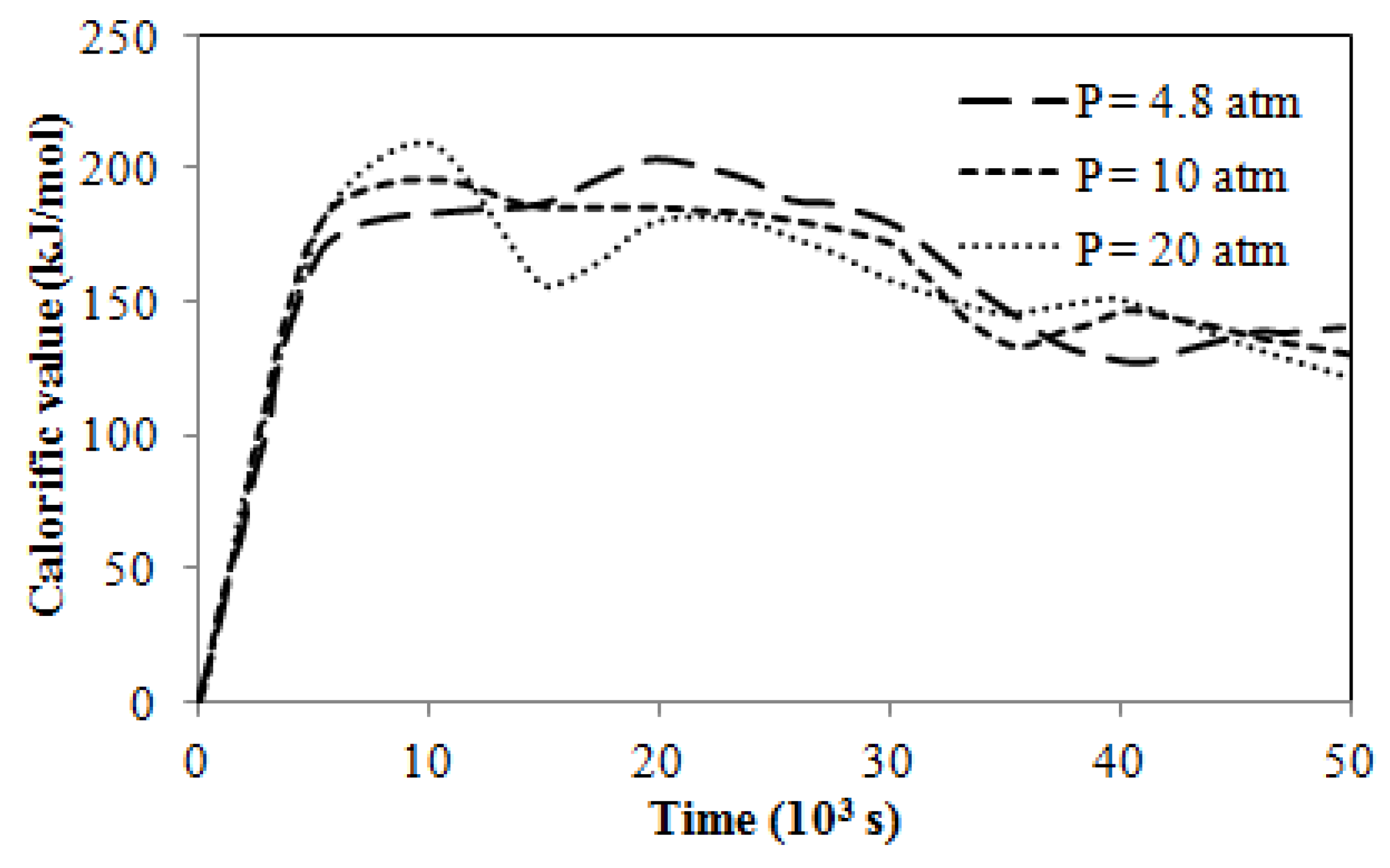
2 ratio, and inlet pressure in their model. They found that increasing oxygen concentration (holding the steam fraction constant) in the feed increases the propagation rate of the reaction front and the temperature in the reaction zone. Similarly, increasing the steam fraction (holding the oxygen concentration constant) increased the propagation rate of the reaction front; however, a decrease in temperature was observed. In the absence of nitrogen, they found an optimum outlet product with a steam/oxygen ratio of 1.5. They also found that input parameters did not influence the pyrolysis reaction. They also reported the variation of the gross calorific value of the exhaust gas, on a dry basis, at different pressures with time (
Figure 9) where the gross calorific value was calculated using the following formula obtained from Harker and Backhurst [
52]:
where
Hi is the heat of the combustion of the gas “i” (kJ/mol), and
yi is the mole fractions of the gas “i” in the product gas on a dry basis. However, the calculation was based on the exit concentration of CO, H
2, and CH
4 only. Pressure was found to have no effect on the process (
Figure 9). In all the cases, a steady flow rate and composition in the outlet was reached after 5000 s of process simulation.
Figure 9.
Gas calorific value at different total pressures with time [
46].
Figure 9.
Gas calorific value at different total pressures with time [
46].
Recently, Uppal
et al. [
43] also developed another 1D packed bed model adopting the existing model of Thorsness
et al. [
48] with some modifications in the model structure and solution strategy. In order to observe their model capability, they considered a bed length of 4.8 m only and observed various features of their simulations with qualitative agreement with the literature. However, for validating their model with the experimental data, they considered the experimental data from their pilot plant which had dimensions of 150 m × 125 m that contained an array (7 × 6) of wells connected by a network of pipes. For comparing with the model calculation, only two consecutive wells that were 25 m apart from each other, were considered.
Table 9 shows their input parameters, some of which are significantly different from the model that they followed.
Table 9.
Input parameters for UCG packed bed model developed by Uppal
et al. [
43].
Table 9.
Input parameters for UCG packed bed model developed by Uppal et al. [43].
| Parameters | Value |
|---|
| Length of Reactor | 25 m |
| Coal Type | Lignite B |
| Injected Gas | Air |
| Injected Gas Flow Rate | 2 × 10⁻⁴ gmole/cm2·s (for observation of model capabilities) |
| Initial Feed Temperature | 430 K |
| Pressure | 6 Atm |
| Initial Coal Density | 1.25 g/cm3 |
In their pilot plant, the injected gas (air only) flow rate was varied with time (
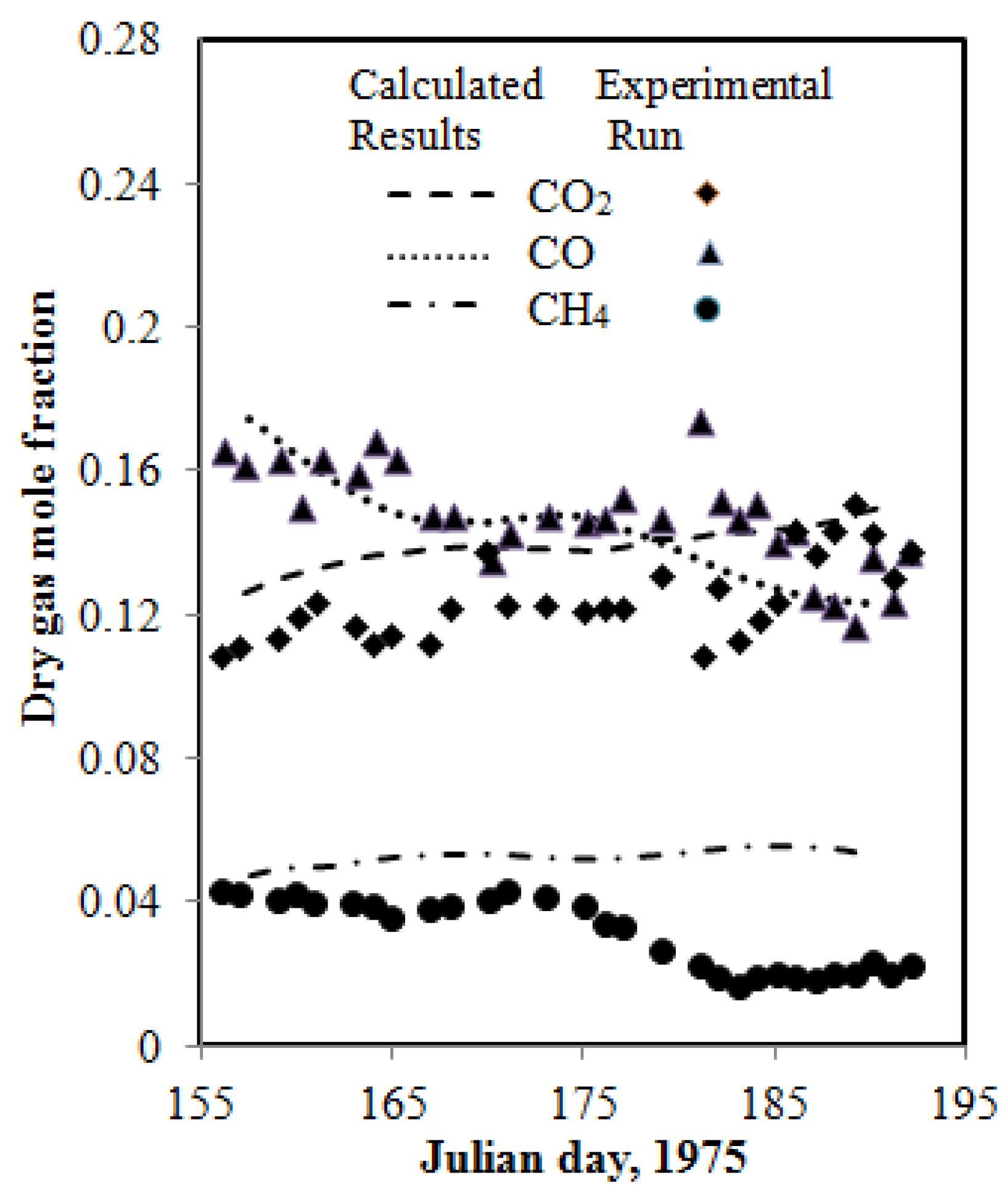
Figure 10) and the resultant heating value and the exhaust gas composition were recorded. In their model, they calculated the exit gas heating value and composition utilizing the experimental inlet gas flow rate. In addition, they used a nonlinear optimization technique in order to compensate the uncertainty in coal and char by optimizing the composition parameters of some pyrolyzed products (H
2, CH
4, and char). The calculated results were in a reasonable agreement with the experimental results (
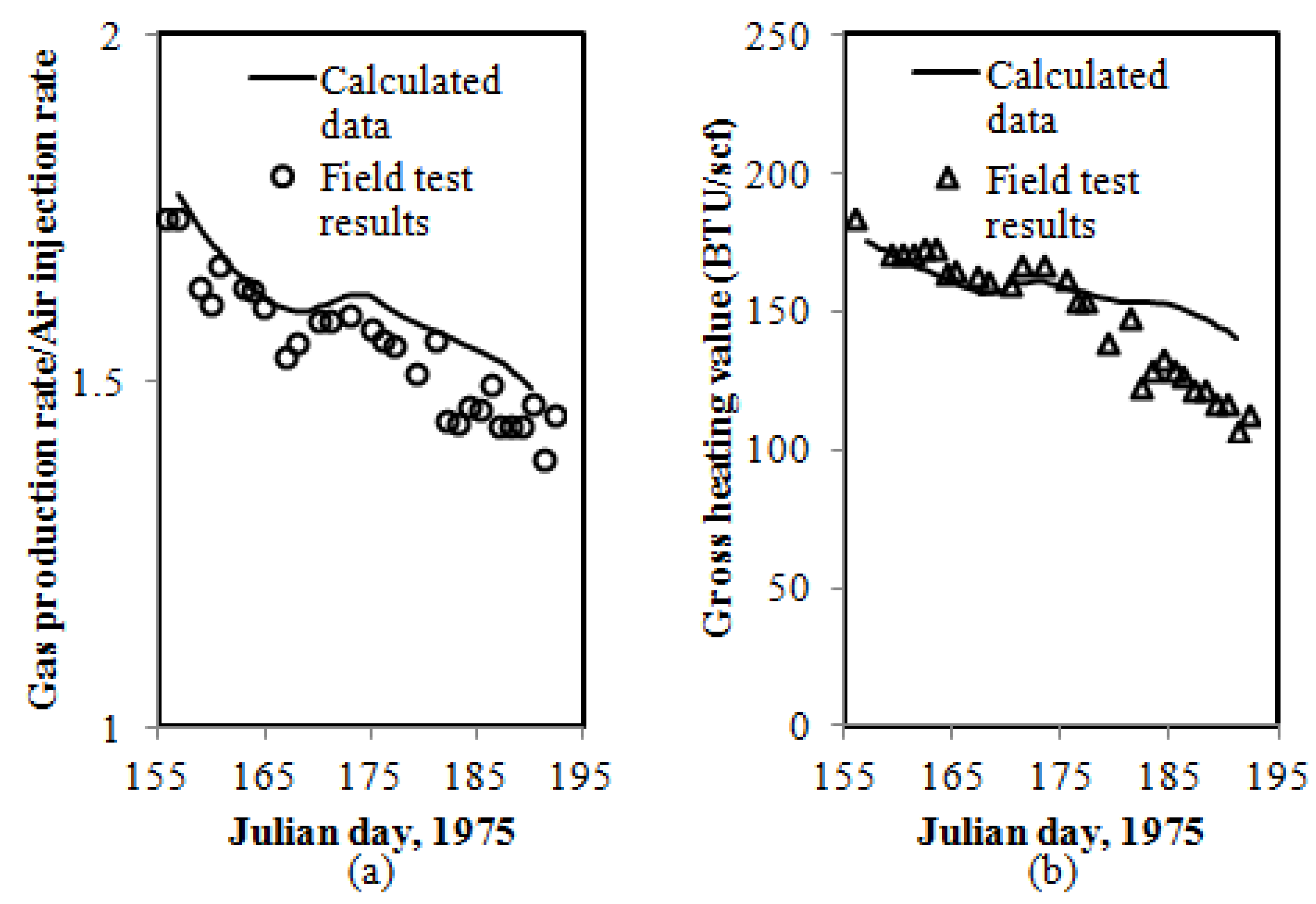
Figure 11a,b). However, according to them, a better prediction can be obtained by increasing the optimization variables. Their model lacks some detailed information such as particle diameter, porosity, permeability,
etc., which are considered important for understanding a UCG process. Nevertheless, their model indicates that a control strategy can be employed by manipulating the inlet flow rate to maintain a desired heating value in the presence of disturbances.
Figure 10.
Flow rate of the injected air with time [
43].
Figure 10.
Flow rate of the injected air with time [
43].
Figure 11.
Experimental and simulated (
a) heating values and (
b) mole fractions of important gases of the product gas mixture with time (reproduced from Uppal
et al. [
43]).
Figure 11.
Experimental and simulated (
a) heating values and (
b) mole fractions of important gases of the product gas mixture with time (reproduced from Uppal
et al. [
43]).
In 1986, Thorsness and Kang [
51] developed a generalized 2D model for describing reacting flows through the packed bed using the following governing equations:
Mass balance:
Conservation of gas species:
Overall solid conservation:
Solid species conservation:
Energy balance:
They assumed an identical gas and solid temperature and incorporated one energy equation for the combination of gas and solid as follows:
Considering the negligible difference between the gas and solid temperature obtained by the earlier models [
47,
48], the assumption of identical gas and solid temperature seems to be justified.
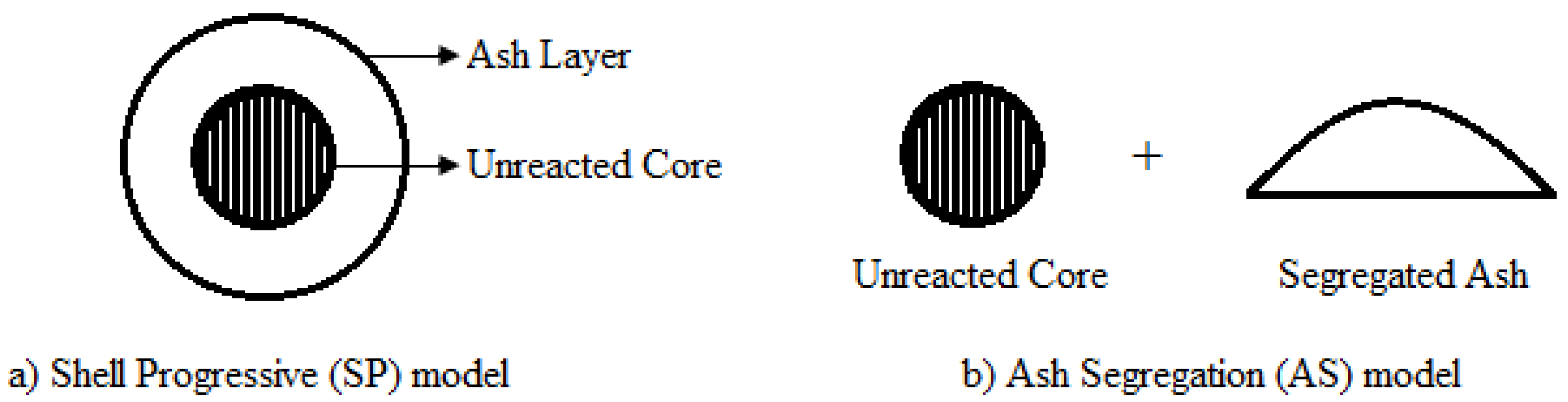
In their model, they incorporated diffusion effects, wall transport, and also char combustion and water-gas shift reaction rates based on Shell Progressive (SP) and Ash Segregation (AS) reaction models. In the SP model, a core of unreacted solid was assumed to be surrounded by a shell of ash through which the gas phase reactants diffuse (
Figure 12a). On the other hand, the AS model assumed continuous exposure of unreacted material to the gas stream due to the ash segregation (
Figure 12b).
Figure 12.
Different reaction regimes in packed bed model.
Figure 12.
Different reaction regimes in packed bed model.
Reaction rates for these two models were as follows:
Because of the generalized nature of their model, they tested various cases (
i.e., transient concentration and thermal wave, steady heat transfer phenomena,
etc.) for non-reacting packing materials through the packed bed and compared them favourably with other available studies. Although their generalized model is 2D, only one case (steady heat transfer phenomena) was solved using the 2D model. For all other cases, the 1D model was considered. For validation of a UCG model, they calculated gas composition, temperature, and carbon fraction considering a steady 1D model with very limited gas species and compared the results with the analytical data obtained from literature. They analyzed the following three disparate situations related to the UCG process which were not considered in the earlier models:
- -
Case 1: Transient water injection into the midpoint of the packed bed during gasification.
- -
Case 2: Coal wall drying using a hot gas flow.
- -
Case 3: Wall regression during gasification.
Table 10 shows the input parameters for the above situations. For the first case, seven gas species (N
2, O
2, H
2, CO, CO
2, water vapor, and CH
4) and eight reactions (reactions 3–11) were considered. However, drying and pyrolysis reactions were ignored. During gasification process, when the product gases reached a reasonably steady state, water was injected at the midpoint of the bed, slightly downstream of the reaction front, and continued until the mole fraction of CO and CO
2 were observed to approach steady values. However, the liquid water influx was assumed to turn into steam instantly with a flow rate of 8 × 10
−4 mol/s. A sudden change in CO and a gradual change in H
2 were noted after the water injection; however, the gases undergoing changes returned to pre-injected conditions as seen in
Figure 13.
Table 10.
Input parameters for the three situations considered by Thorsness and Kang [
51].
Table 10.
Input parameters for the three situations considered by Thorsness and Kang [51].
| Input Parameters | Case 1 | Case 2 | Case 3 |
|---|
| Packed Bed Dimension | L = 150 cm, D = 5 cm | L = 25 cm, D = 10 cm | L = 1 m, D = 1 m |
| Initial Gas Temperature | 900 K | 900 K | 900 K |
| Initial Bed Temperature | | 300 | |
| Gas Composition | |
| H2O | 74% | 100% (or N2) | 66.6% |
| O2 | 26% | | 33.3% |
| Injected Gas Flow Rate | 1.5 × 10⁻³ mole/s | 8 × 10⁻³ mole/s
(1 mol/s-m2 of bed) | 6 moles/s |
Figure 13.
Product gas changes during gasification with midpoint water injection [
51].
Figure 13.
Product gas changes during gasification with midpoint water injection [
51].
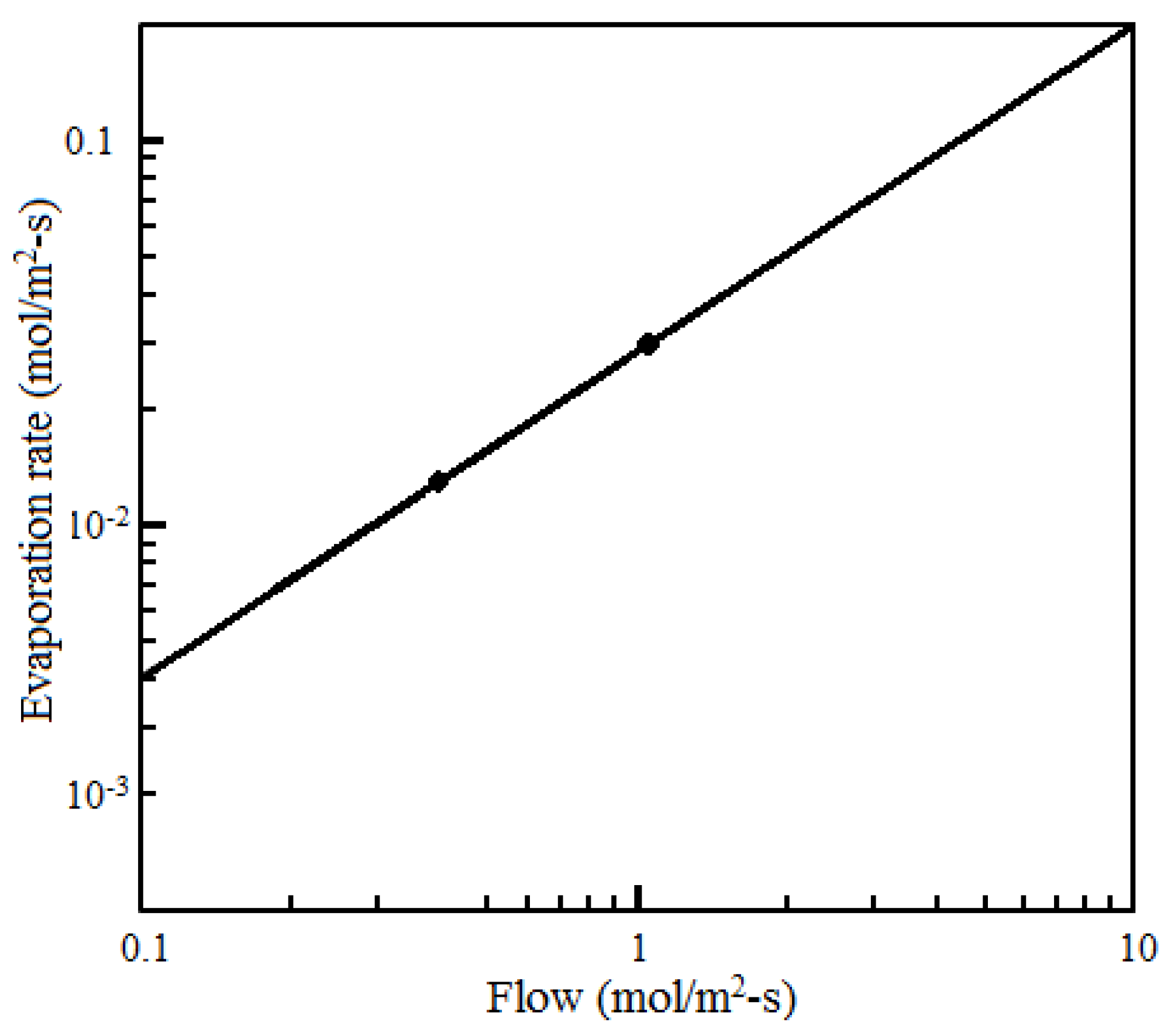
For case 2, a uniformly permeable non-reacting bed with a water-saturated wall at steam temperature was assumed through which hot gas was passed. It was observed that the time to reach steady state increased rapidly with a decreasing flow rate as if the average wall-drying rate is a function of the injected gas flow (
Figure 14). However, the wall-drying rate was found to be limited by the available energy for too low injected hot gas due to the insufficiency of the total heat injected.
Figure 14.
Drying rate
vs. flow rate (log-log plot, from Thorsness and Kang [
51]).
Figure 14.
Drying rate
vs. flow rate (log-log plot, from Thorsness and Kang [
51]).
For case 3, the model system was considered to be filled with rubble material consisting of ash in the center and char near the walls and at the top. The walls were considered as coal that can proceed with gasification reactions. The objective of this model system was to determine the thickness of the char bed at the wall that would lead to a self-sustaining system. Calculations were performed using all seven gas species. The computed wall regression rate (
i.e., the carbon production rate) was found nearly constant with the increasing char layer thickness, while the carbon consumption varied linearly with the char thickness (
Figure 15). A wall char bed thickness of 7.5 cm was found close to a self-sustaining system, since the rate of carbon consumption was nearly equal to the carbon production. However, the calculated average wall regression rate of 7.7 × 10
−7 m/s (0.07 m/day), when comparing the characteristic field result (~0.5 m/day), indicates that their model is missing some additional physics.
Figure 15.
Carbon production rate
vs. wall char layer thickness [
51].
Figure 15.
Carbon production rate
vs. wall char layer thickness [
51].
In 1976, in parallel to LLNL, Gunn and Whitman [
45] also developed a 1D linear mathematical model separately for UCG. Their work is particularly important as their model is the only packed bed model cited in the literature that was compared with the field trials (Hanna, Wyoming) and exhibited a fairly good agreement with the experimental data (
Table 11). However, field test data was considered at a time span when a steady-state condition was observed in order to conform closely to the assumption of their model. In addition to the gas composition, temperature, and heating value, they also determined the ratio of the gas production rate to the gas injection rate, the effect of reservoir water influx on the heating value of gas, the distribution of thermal energy and thermal efficiency during the gasification process that closely matched the experimental observations and, thus, provided enhanced understanding of the UCG process.
Table 11.
Comparison of experimental and calculated data for an air injection rate = 1631 Mcf/day [
45].
Table 11.
Comparison of experimental and calculated data for an air injection rate = 1631 Mcf/day [45].
| Components | Composition (Mole Percent) |
|---|
| Field Test Results | Calculated Data (Average Value) |
|---|
| H2 | 18.57 | 18.60 |
| CH4 | 4.10 | 4.92 |
| N2 + Ar | 47.81 | 47.13 |
| CO | 16.35 | 15.83 |
| CO2 | 12.33 | 13.29 |
| H2S | 0.04 | 0.07 |
| Ethan + | 0.80 | 0.14 |
| Gas Production Rate (Mcf/day) | 2728 | 2734 |
| Gas Production Temperature, °F | 493 (measured at the surface) | 533 (measured at the bottom of the well) |
| Maximum Temperature, °F | 1871 | 1951 |
| Heating Value, Btu/scf | 170.6 | 164.6 |
| Thermal Efficiency (%) | 89.2 | 87.4 |
Unlike the above models, the water-gas shift reaction and methanation were not included in their model. Methane was considered to be produced solely through pyrolysis. Only two reactions, water-gas and combustion reactions, were considered. The reaction rate of the water-gas reaction was adopted from the work of Gadsby
et al. [
53]; however, the constants were determined from the gasification of the pitch coke. For the combustion reaction, the reaction data of Lewis
et al. [
54] was used that was obtained from the combustion of metallurgical coke. Even the correlation of the thermal conductivity they used was not intended for subbituminous coal. Drying was not considered in their model. Despite this and the large errors in the reaction rate, they observed only negligible errors in the model predictions.
In their model, water vapor, carbon monoxide, hydrogen, carbon dioxide, oxygen, inert gases (nitrogen and argon), and devolatilized material from the coal were considered. For convenience, the volatile products resulting from the pyrolysis of coal were treated as a single pseudocomponent; however, the pseudocomponent was broken down into individual gases for the purpose of calculating total gas composition. From the proximate and ultimate analysis of the experimental subbituminous coal (from the Hanna field test), they also formulated a correlation between the weight fraction of volatile matters and the temperature with high accuracy. In order to obtain the composition of devolatilized gas, they considered the experimental devolatilized data of the Hanna I coal seam at 900 °C along with the assumption that the tars (16.2%) and light oil (0.9%) and water (13.3%) in that analyses cracked to the stoichiometric proportion of methane, carbon monoxide, and hydrogen. Their assumption led to the composition for devolatilized products listed in
Table 12.
Table 12.
Composition of devolatilized products assumed by Gunn and Whitman [
45].
Table 12.
Composition of devolatilized products assumed by Gunn and Whitman [45].
| Components | Percent |
|---|
| H2 | 42.26 |
| CO | 28.53 |
| CO2 | 3.79 |
| CH4 | 24.36 |
| H2S | 0.37 |
| Ethane + | 0.69 |
| Total | 100 |
| Average molecular wt. | 14.76 |
Their model transformed the set of partial differential equations into a set of ordinary differential equations by considering the pseudo-steady-state approximation. They considered nine integrated continuity equations (two for overall solid and mass balances and others for individual gas species), a partially integrated energy equation, and a macroscopic material balance equation from which a constant combustion front velocity could be calculated iteratively. The assumption of the constant combustion velocity seems to be valid, according to
Figure 6, with what was observed by Thorsness
et al. [
48].
Their model predicted the exhaust dry gas composition and obtained a close agreement with the experimental gas composition history with the exception of methane (
Figure 16). However, the deviation of methane was believed to be a result of considering a high concentration of methane in the devolatilized products. The only parameter fitted in their model from the field trial was the water influx in order to get a good prediction for the data that interferes with the water influx rate. Their calculated results were also closely matched with experimental data for ratio of gas production/air injection and gross heating value (
Figure 17 and
Figure 18). However, the declination of those quantities with time was believed to be the result of the gradual increase of water flux during field test. They calculated the heating value of gas by changing the ratio of water influx to air injection rate and observed a maximum heating value at a ratio of about 0.15. Usually the maximum heating value at a particular ratio of water intrusion to air injection rate implies the control strategy of closely maintaining the optimum value either by controlling the water intrusion rate by pressure of any other means or by changing the air injection rate.
Figure 16.
Comparison of calculated exhaust gas compositions from Gunn and Whitman [
45] with experimental results from the Hanna field trial.
Figure 16.
Comparison of calculated exhaust gas compositions from Gunn and Whitman [
45] with experimental results from the Hanna field trial.
Figure 17.
Comparison of calculated data and field test: (
a) gas production/air injection ratio and (
b) gas heating value [
45].
Figure 17.
Comparison of calculated data and field test: (
a) gas production/air injection ratio and (
b) gas heating value [
45].
Figure 18.
Effect of reservoir water influx on heating values of gas [
45].
Figure 18.
Effect of reservoir water influx on heating values of gas [
45].
The calculated values of the distribution of thermal energy released by coal combustion were also in good agreement with the experimental values (
Table 13). From the experimental data, it was observed that only a small amount of energy from a 30-foot coal seam was lost to the overburden and base rock. This implies that neglecting heat losses to the surrounding rocks does not hamper a model outcome too much. The last column of
Table 13 shows a higher heating value of the product gas when injected air was preheated at 480 °F. In order to get higher economic value and energy conservation, they suggested using a part of the heat of vaporization of the produced water to heat the inlet gas. They also reported that in all cases, the reaction zone was very narrow, generally two feet or less. This fact was verified by both model calculations and by temperature measurements in the observation wells.
Table 13.
Distribution of thermal energy from
in situ coal combustion [
45].
Table 13.
Distribution of thermal energy from in situ coal combustion [45].
| | Calculated, % | Field Test, % | Calculated with Preheating, % |
|---|
| Produced Gas | | | |
| Gross heating value | 87.4 | 89.1 | 91.3 |
| Sensible heat.... | 5.8 | 5.2 | 2.9 |
| Heat of vaporization of water vapor in produced gas | 3.4 | 3.3 | 2.4 |
| Heat Loss to Surrounding Rock | 1.3 | 3.8 | 1.3 |
| Heat Loss in Ash | 2.1 | 0.6 | 2.1 |
| Total | 100 | 100 | 100 |
Although they obtained a good agreement with the experimental results for a number of phenomena, they could not quantitatively predict the variation of the temperature and mole fraction along the bed length with the experimental value because of the poor consideration of the thermal conductivity, heat capacities, and the uncertain accuracy of the reaction rates. However, they obtained a qualitative agreement with the experimental values. Despite very close agreement with the experimental data, their model is not sufficient for predicting all aspects of gasification as their model neglected some important phenomena, such as drying, CO2 gasification, the water-gas shift reaction, gas phase reactions, etc. However, because of the low water/air ratios that were experienced with the Hanna tests, there might be little or no water-gas shift reactions. As a result, the Gunn model was not hampered by neglecting this reaction. In their model, there is also a lack of sensitivity analysis for the kinetic parameters they used. In addition, they included water influx data from a particular field trial. However, water influx is a highly variable phenomenon that depends on coal seam properties and hydrology. All these lacking parameters limit their model for general applicability in the UCG process.
Abdel-Hadi and Hsu [
8] extended previous models by developing pseudo-2D geometry with a moving burn front in the axial direction. A rectangular domain with a length of 1.5 m and width of 1 m was used in their model. Their governing equations are nearly similar to the equation considered by Winslow [
47] and Thorsness and Kang [
51]; however, they included carbon consumption in the reaction zone in order to track the burn front, and the equation is given by:
where
wc is the carbon mass fraction,
vc is the velocity of the combustion front, and
xrz is the total length of the reaction zone. They also performed an immobilization transformation of coordinates in order to formulate the irregular front motion as follows:
All other governing equations were transformed to these new coordinates (
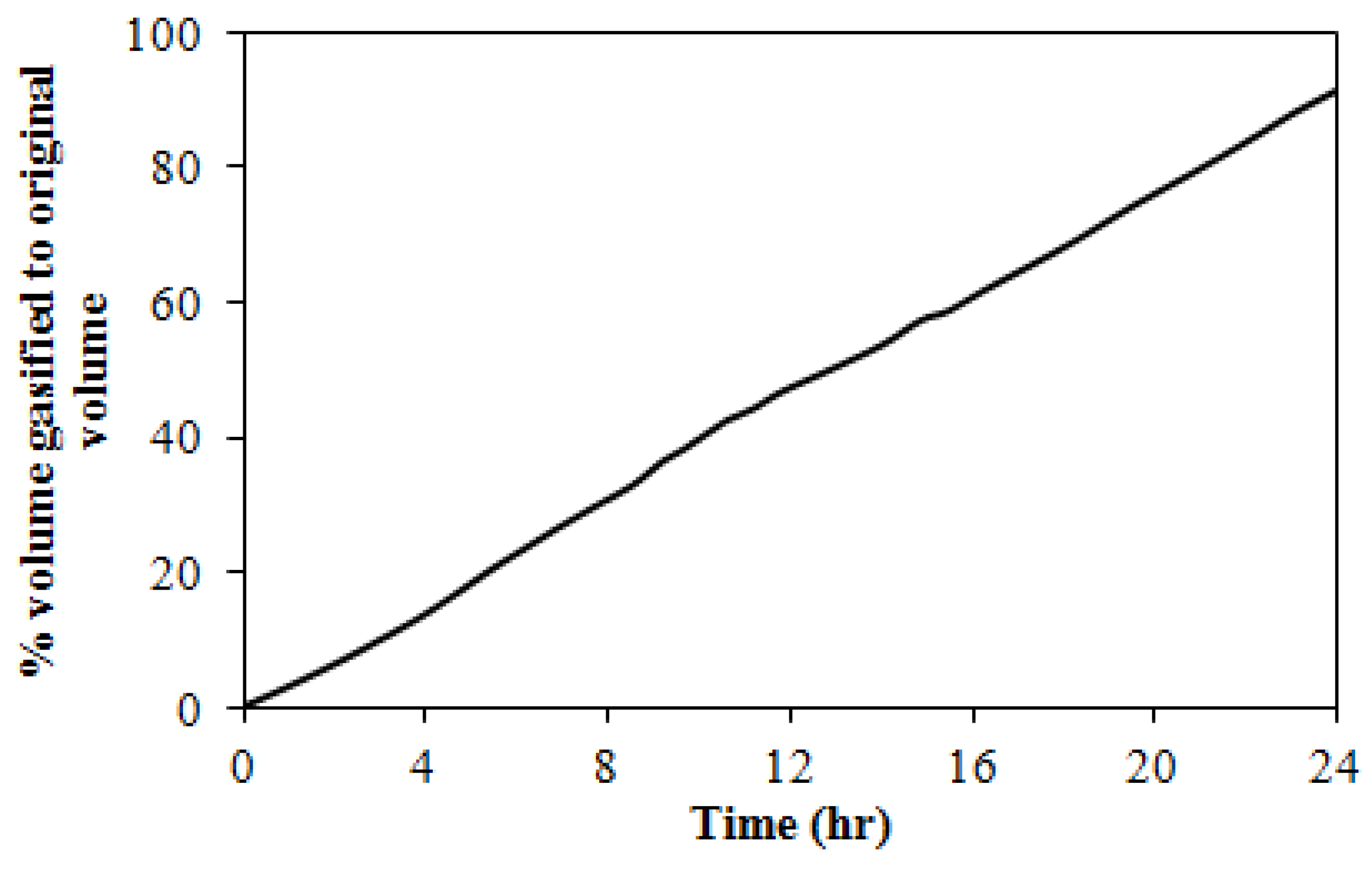
Figure 19). This allowed them to calculate the progressive configuration of the gasified zone at various stages of gasification (
Figure 20) which, in turn, facilitated the calculation of the rate of coal seam consumption (
Figure 21). The conversion rate of the coal seam is found fairly constant. In order to gain confidence for this model, they have compared their model with the laboratory results reported by Thorsness and Rozsa [
42] and obtained a good agreement with the experimental data.
Figure 19.
Schematic description of the problem: (
a) conventional coordinate system; (
b) immobilization coordinate system (redrawn from Abdel-Hadi and Hsu [
8]).
Figure 19.
Schematic description of the problem: (
a) conventional coordinate system; (
b) immobilization coordinate system (redrawn from Abdel-Hadi and Hsu [
8]).
Figure 20.
Progressive configurations of combustion fronts during gasification [
8].
Figure 20.
Progressive configurations of combustion fronts during gasification [
8].
Figure 21.
Consumption of coal during gasification [
8].
Figure 21.
Consumption of coal during gasification [
8].
The packed bed models have been validated with laboratory experiments to some extent. These models exhibit good agreement for the gas composition. In order to calculate the heat recovery and gas composition, the model can be very effective. However, the extension of these models to field trials is infeasible, since other cavity growth mechanisms such as thermo-mechanical failure could not be incorporated into the models. Also, as pointed out by Winslow [
47], this method requires a fine grid at the vicinity of the reaction front that limits its applicability to three-dimensional field-scale trials. However, recent advancement of computational power can easily overcome this limitation.
2.2. Channel Models
Beside packed bed models, a number of channel models have also been developed in the first decades of modeling. The channel model assumes that coal is gasified only at the perimeter of the expanding permeable channel [
19]. In this approach, the UCG process is represented by an expanding channel when two distinct zones of rubble/char and open channel exist. This approach is considered due to the observation of the formation of the open channel structure after the gasification phase is terminated in different field tests of coal seams [
55,
56].
Figure 22 shows the basic concept and physics behind this approach: “Air or oxygen flows down the central channel and is convected by turbulent flow to the boundary layer along the channel wall. The oxygen diffuses through the boundary layer to the solid surface and reacts. The hot combustion gases diffuse back through the boundary layer to the channel” [
40]. The channel model is more useful for analyzing sweep efficiency [
19].
Table 14 and
Table 15 represent a glimpse of a list of channel models discussed here with their essential features and reaction rate control mechanisms of the main reactions in the gasification process, respectively.
Figure 22.
Reactions and transport phenomena in channel model (redrawn from Gunn and Krantz [
40]).
Figure 22.
Reactions and transport phenomena in channel model (redrawn from Gunn and Krantz [
40]).
Table 14.
Some essential features of reported channel models.
Table 14.
Some essential features of reported channel models.
| Researchers | Dimension and Time Dependence | Heat Transfer | Mass Diffusion | Fluid Flow | Thermo Mechanical Failure | Water Influx | Heat Loss |
|---|
| Conduction | Convection | Radiation |
|---|
| Dinsmoor et al. [44] | 2D and T | √ | √ | √ | | P | | √ | |
| Eddy and Schwarz [57] | 1D and T | √ | √ | √ | √ | M | √ | √ | √ |
| Luo et al. [58] | 2D and T | √ | √ | | √ | | | | |
| Batenburg et al. [55] | 1D and SS | √ | √ | √ | | D | | | |
| Pirlot et al. [59] | 2D and S | √ | √ | | √ | D | | √ | |
| Kuyper [56,60] | 2D and T | √ | √ | √ | √ | NS | | | |
| Perkins and Sahajwalla [61] | 2D and T | √ | √ | √ | √ | NS | | | |
Table 15.
Reaction rate control mechanisms of the main reactions in the gasification process.
Table 15.
Reaction rate control mechanisms of the main reactions in the gasification process.
| Researchers | Drying | Pyrolysis | Char Reaction | Water-Gas Shift Reaction | Gas Phase Reaction |
|---|
| C + O2 → CO2 | C + CO2 → 2CO | C + H2O → CO+ H2 | C + 2H2 → CH4 | CO + H2O↔ CO2+ H2 | CO + 0.5O2 → CO2 | H2 + 0.5O2 → H2O | CH4+2O2→ CO2+2H2O |
|---|
| Dinsmoor et al. [44] | | | K | K | K | | | P | P | |
| Luo et al. [58] | | | P | P | P | P | P | P | P | P |
| Batenburg et al. [55] | | | | E | E | E | E | | E | |
| Pirlot et al. [59] | | | | E | E | E | E | E | E | E |
| Kuyper [56,60] | | | | D | | | | M | | |
| Perkins and Sahajwalla [61] | | | | P | | | | M | | |
Dinsmoor
et al. [
44] developed a steady-state, 1D channel model by assuming that the gasifier behaves as an expanding cylindrical cavity in the coal seam with reactions taking place at the walls. In their model, for simplicity, no pyrolysis reactions were considered. Heat transfer included conduction for solids only; however, both convection and radiation were included between the wall and gas. Axial heat conduction in the gas phase was neglected. They also considered water influx as evenly distributed along the length of the tube. Char reactions (reactions 3–5) and two gas phase reactions (reactions 9 and 10) were considered in their model. Because of slow channel evolution, they incorporated a pseudo-steady-state assumption for changes associated with the gas phase. They treated a fully developed flow process with the channel despite the initial cylindrical channel diameter (0.3 m) being much smaller than the channel length (60 m). Considering forced convection as the dominating mechanism of mass transfer, they simulated coal gasification with a forced convection mass transfer correlation. For heterogeneous reaction kinetics, they considered the surface reaction rate constant and wall diffusion resistances. For wall diffusion resistances, the mass transfer coefficients were calculated from a standard correlation for the turbulent flow of gases in tubes. Inlet gas was assumed to be air at 330 K and 6.9 atm with no water added. Their predicted gas compositions and temperature profile showed clear evidence of the presence of a separate oxidation and reduction zone; however, a very high temperature (2400 K) was noted near the inlet (
Figure 23). According to them, this high temperature was due to neglecting heat loss at the end of the tube and including the radiation heat transfer. However, it appears that apart from their explanations, neglecting the pyrolysis reaction could be another reason for getting high temperature initially, as during ignition, a significant amount of heat is used to create char by the pyrolysis of coal.
Figure 23.
Typical channel temperature (gas and wall) and gas composition profiles without water influx [
44].
Figure 23.
Typical channel temperature (gas and wall) and gas composition profiles without water influx [
44].
The quality of the predicted product gas observed was inferior to the gas quality usually obtained in the packed bed model for similar situations. For a constant blast velocity, the reaction rates were observed to decrease with the evolution of the channel due to the constant mole fraction of the oxygen. As a result, the oxidation zone became longer which, in turn, was responsible for increased heat losses and the deterioration of gas quality. Compared to the packed bed combustion front (approximately 0.2 m), the oxidation zone (approximately 20 m) was much longer. However, these observations were not supported by any field observations. Apparently, because of the long oxidation and reduction zones, they concluded that “a successful UCG system cannot be operated in the channel regime”.
Almost at the same time, the above conclusion was negated by the work of Schwartz
et al. [
62] as they found an increase of mass transfer by several orders of magnitude when natural convection in channels was considered as the controlling mechanism of mass transfer instead of forced convection alone. The intense mixing of the injected blast with the boundary layer gases depends on the Grashof number (Gr) of the natural convection flow. A good mixing begins when the Grashof number exceeds 10
8 and becomes intense at about 10
10 [
63]. However, for dominant natural convection flow, the gases within the boundary layer produce a circulatory flow within the cylinder and a good mixing is obtained. However, Schwartz
et al. [
62] assumed two different modes of the circulatory pattern based on coal seam thickness as depicted in
Figure 24.
Figure 25 shows the difference of cavity growth with and without considering the natural convection. Later, it was established by mathematical correlation that the models assuming forced convection mass transfer as the controlling mechanism for cavity growth were not born out of field trials [
15].
Figure 24.
Assumed circulation patterns in the thick seam and thin seam configurations (redrawn from Schwartz
et al. [
62]).
Figure 24.
Assumed circulation patterns in the thick seam and thin seam configurations (redrawn from Schwartz
et al. [
62]).
Figure 25.
A comparison of cavity growth via forced convection and natural convection [
62].
Figure 25.
A comparison of cavity growth via forced convection and natural convection [
62].
Schwartz
et al. [
62] were the first investigators to consider the natural convection as the controlling mechanism of heat and mass transfer in UCG cavities. In their later paper, Eddy and Schwarz [
57] developed a 2D model and described the evolution of the cavity based on the movement of the cavity wall. The blast from the injection well was transported through the reacting walls of a constant temperature via the convection process and ultimately diffused to the wall and reacted with the coal. The oxygen diffusion rate was calculated by natural and forced convective heat and the mass coefficient. The roof and floor of the cavity were assumed to be non-reacting surfaces. They considered neither subsidence nor rubblization. They included the water-gas shift reaction and two other gas phase oxidations along with three char reactions (reactions 3–5) as considered by Schwartz
et al. [
62]. In order to capture the experimentally proven teardrop shape of the cavity formation, they divided the cavity growth into different regions,
i.e., a hemispherical region in the vicinity of the injection well and a series of non-equal diameter cylinders (step cylinder) downstream from the injection well, according to the flow process and a cylindrical link zone (
Figure 26). At any location, the cavity was assumed to be a cylindrical cross-section until the cavity diameter was equal to the seam thickness, which is when the model switches to a rectangular cross-section. It was assumed that all coal volume located in the hemispherical region was consumed in the reaction with oxygen. The volume of char was calculated from the mass of char burned due to the combustion and the density of the char. The half-body volume was then fit to the calculated char volume. Flow was treated as an entrance region of pipe, as the calculated entrance length was much larger than the vertical well distance. The entrance length was calculated using the following equation:
where
Le is the entrance length and
d is the pipe diameter. The minimum Reynolds number in the system was 4000, which resulted in an entrance length of 48.8 m. The entrance length was considered to increase with the increase of the cavity diameter. According to them, as fresh blast proceeds down the axis and products of combustion are released at the walls, the forced and natural convection results in a swirling flow that ultimately helps mix the flows and enhance the flow of oxygen to the vicinity of the wall where boundary layer convective diffusion dominates. The transport of heat and species inside the cavity was considered to be governed by empirical correlations for the turbulent transport phenomena in enclosures. The model was able to reproduce the results of the Hanna II and Pricetown field trials qualitatively.
Figure 26.
Conceptual sketch of the linked vertical well computer model geometry (redrawn from Eddy and Schwarz [
57].
Figure 26.
Conceptual sketch of the linked vertical well computer model geometry (redrawn from Eddy and Schwarz [
57].
Recently, Luo
et al. [
58] extended the Schwartz
et al. [
57] model by including heat transfer and more coal wall and gas phase reactions (reactions 3–10). Flow inside the cavity was solved based on irrotational fluid flow inside an enclosure, which describes velocity potential based on geometric features of the enclosure. The geometry is shown in
Figure 27. The stream function and velocity potential were calculated using the following equations:
Velocity potential:
where
U is the velocity of the uniform stream and
ṁ is the mass flow rate. Pressure distribution in the cavity was determined using Bernouli’s equation:
Figure 27.
UCG cavity defined in the work of Luo
et al. [
58].
Figure 27.
UCG cavity defined in the work of Luo
et al. [
58].
In the Luo model, Fluent was used to predict the cavity shape at different times based on heterogeneous reaction rates at the cavity wall. In order to quantify the turbulent intensity, they used the standard k-ε model for the turbulent kinetic energy and dissipation. For heterogeneous and homogeneous reactions, they used kinetics/the diffusion control process and a finite rate/eddy dissipation model, respectively. Their model was validated with Chinchilla field trials. The calculated coal consumption closely matched the Chinchilla trial field data (
Figure 28). For sweep cavity geometry, their model was further validated with the data from the Hanna II and III UCG trials. There is less than 5% error between the results generated with the model (Hanna II: 2436.6 tons of coal gasified in 25 days; Hanna III: 4139.3 tons in 38 days) and reported data (Hanna II: 2500 tons of coal gasified in 25 days; Hanna III: 4200 tons in 38 days). Their model predicts a hemispherical shape for the cavity geometry; however, the model is limited since heat and mass transfer characteristics of the cavity are unknown. Also, the coupling of this model with the mechanical failure of the coal would be cumbersome, since the accumulated rubble in the cavity changes the transport phenomena inside the cavity.
Figure 28.
Coal consumptions for modeling and Chinchilla trial data [
58].
Figure 28.
Coal consumptions for modeling and Chinchilla trial data [
58].
Batenburg
et al. [
55] developed a semi-steady-state 2D model for UCG in open channels for the developed gasifier only. Unlike other models, they assumed that oxygen instantaneously reacts with the combustible gases present in the channel instead of reacting with the coal surface. Their interest was only to investigate the process within the channel after the injection gas percolates through the inert permeable rubble zone. Reaction rates were calculated based on resistances in the system including boundary layer, pore diffusion, surface phenomena, and chemical kinetics. For laminar and turbulent natural convection along a smooth vertical wall, they used the Sherwood number (Sh) that is correlated with the Grashof number (Gr) and Schmid number (Sc) as follows:
For forced convection-dominated flow the Sherwood number was expressed in terms of the Reynolds number (Re) as follows:
Heat transfer was modeled by radiation between the walls of the channel. They also included the effect of natural convection due to the temperature difference. Their results showed that the effect of pressure on gas composition is negligible (
Figure 29). Their results also indicated that natural and forced convection transfer coefficients are in the same order of magnitude and both of them are important.
Figure 29.
Net fluxes and temperature as a function of process pressure for oxygen injection rate = 0.1 mol/m/s and water injection rate = 0.05 mol/m/s [
55].
Figure 29.
Net fluxes and temperature as a function of process pressure for oxygen injection rate = 0.1 mol/m/s and water injection rate = 0.05 mol/m/s [
55].
Pirlot
et al. [
59] developed a 2D steady-state model by extending the idea of Batenburg
et al. [
55] with two distinct zones: a low-permeability rubble and ash around the injection point and a high-permeability peripheral zone along the coal wall (
Figure 30). After a short transitory starting phase, those two zones were identified by other researchers [
64,
65] for a thin seam at great depth. During initial combustion, a cavity was identified partially filled with inert materials near the injection hole [
64,
65]. Their simulation for cavity evolution was based on one main parameter, the permeability ratio between the low- and high-permeability zones. The gasifying agent was assumed to pass through the low-permeability zone surrounding the injection point prior to its arrival in the high-permeability zone, where reactions with the coal wall occur. They combined two separate models: (1) a flow model for the calculation of the flow through the low-permeability porous zone using Darcy’s law and the continuity equation; and (2) a chemical model for the calculation of the chemical processes occurring between gas and the coal wall in the high-permeability zone using empirical correlations for mass and heat transfer for the packed bed by assuming plug flow in the gas phase. The coal consumption rate was calculated only on the channel wall. Their model did not consider the details of moisture and volatile matter released by drying and pyrolysis. They assumed that volatile matter is released in the form of water and hydrogen in proportion to the consumption rate of carbon. They concluded that the permeability ratio is one of the main parameters for determining the success of underground coal gasification because of the observation of the increasing final gasifier area, power, and trial duration with the increase of the permeability ratio. According to them, the cavity growth and shape obtained from their model were in reasonable agreement with the Pricetown field trials.
Figure 30.
Conceptual sketch of the two separate zones and species flow direction (redrawn from Pirlot
et al. [
59]).
Figure 30.
Conceptual sketch of the two separate zones and species flow direction (redrawn from Pirlot
et al. [
59]).
Kuyper [
56,
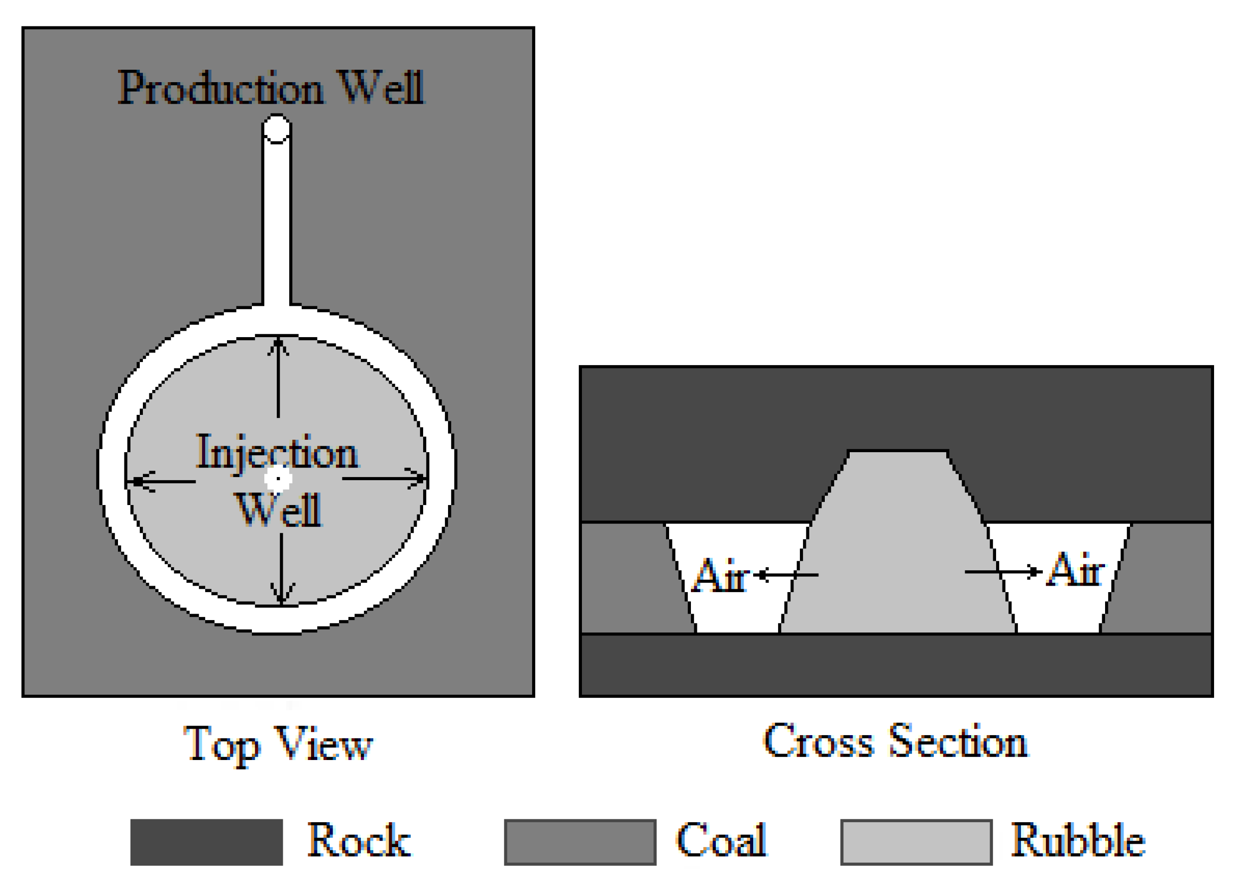
60] developed a 2D model to describe UCG process in a cross-section of an open channel (
Figure 31) for a typical western European coal layer of thin seams (1–2 m). Field trials of UCG indicated the growth of the cavity upwards and radially outwards around the injection well as gasification proceeds [
66]. As a result, at thin seams, the top wall is exposed to rock materials and failure of the overburden is apparently expected. Such a failure would create open channels around the rubble materials deposited on the floor just about the injection hole; as shown in
Figure 31. Considering this fact, in their model, the top and bottom walls were assumed as impermeable and adiabatic rock materials. However, the main focus of their work was to obtain an insight for heat and mass transfer due to double-diffusive turbulent natural convection in which both the temperature and concentration gradients play a role in the transport process. The justification of using double-diffusive turbulent natural convection was based on the expectation that Gr/Re
2 >> 1, considering the Grashoff number (Gr) of the natural convection flow in the process is approximately 10
10 while the Reynolds number (Re) of the forced convection flow is about 10
4. In this situation, if the forced convection flow is superimposed on the natural convection flow, the heat and mass transport phenomena inside the cavity will be dominated by double-diffusive natural convection and a spiral flow can be expected. The justification for this assumption can be found elsewhere [
67]. The Navier-Stokes equation and the
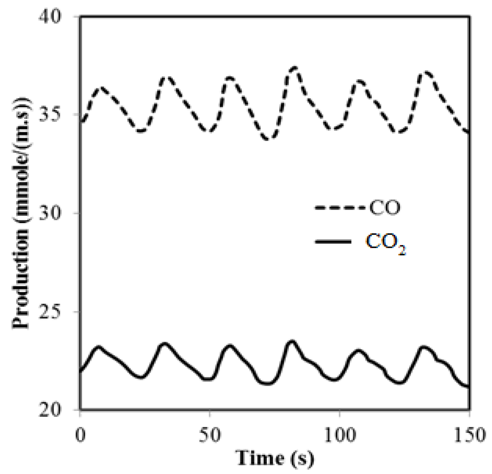
k-ε turbulence model were used to describe fluid flow due to large gradients of density and concentration in the channel. Radiation and convection were assumed to be the major heat transfer mechanisms in the channel. Model results showed that oxygen is consumed far from the coal wall by combustible gases. The double-diffusive natural convection in the channel was observed to cause the periodic generation and collapse of CO
2 bubbles (
Figure 32). Also, mass transfer was reported to be the controlling mechanism (the rate-limiting step) for reduction reactions at the coal wall. They also studied the effect of CO
2 injection into the coal seam and reported that CO
2 injection has a similar effect as adding steam, although to a lesser extent.
Figure 31.
Channel formation in thin seams (Modified from Kuyper
et al. [
60]).
Figure 31.
Channel formation in thin seams (Modified from Kuyper
et al. [
60]).
Figure 32.
Production of CO and CO
2 as function of time for κ = 0.12 m
−1 and an oxygen injection rate of 47 mmole m
−1s
−1 [
60].
Figure 32.
Production of CO and CO
2 as function of time for κ = 0.12 m
−1 and an oxygen injection rate of 47 mmole m
−1s
−1 [
60].
Because of the identification of UCG application in thick coal seams and the presence of a porous bed of ash overlying the injection point and a void space above the UCG cavity based on field trial excavation [
66,
68,
69] as depicted in
Figure 33, Perkins and Sahajwalla [
61] considered a thick coal seam and expanded Kuyper’s model by including an ash layer at a lower part of the channel (
Figure 34). They developed a 2D axisymmetric model by using Fluent to investigate double-diffusive natural convection along with relevant reactions in a partially filled cavity. Although the bottom wall was considered to be inert and adiabatic, the side and top walls were considered to be carbon due to the thick coal seam. The temperature of the gas and the porous ash bed were assumed to be in thermal equilibrium. The flow though the porous ash bed was modeled using a laminar approximation; however, the turbulence model is only applied to the void region of the cavity. The low Reynolds number turbulence model of Launder and Sharma [
70] was employed for the turbulent model by replacing the constants in the standard
k-ε model with the function of the turbulent Reynolds number in order to extend the model’s applicability to low-turbulence regions that are close to walls. The following turbulent kinetic energy (
kt) and the turbulent dissipation rate (
ε) equations were used in order to account for turbulent intensity:
Figure 33.
Schematic of an underground coal gasification cavity from field observation (redrawn from Perkins and Sahajwalla [
61]).
Figure 33.
Schematic of an underground coal gasification cavity from field observation (redrawn from Perkins and Sahajwalla [
61]).
Figure 34.
Channel geometry in Perkins and Sahajwalla [
61].
Figure 34.
Channel geometry in Perkins and Sahajwalla [
61].
For other conservation equations for void space, they followed the standard governing equations developed for porous media with the exception of φ (porosity) = 1. For the simplicity of their model, only three chemical reactions (reactions 2, 8, and partial char combustion) were considered. They found that the flow behaviour in the void space is dominated by a single buoyant force due to the temperature gradient resulting from the combustion of oxygen with CO produced from the gasification of CO
2 at the walls. From the observable entity, by changing the injection point, they concluded that oxygen should be injected at the bottom of the channel, otherwise valuable gasification products would be oxidized, leading to a low heating value of the production gas. The model was verified with Biezen’s experiments [
71] for double-diffusive natural convection in a trapezoidal channel.
Considering the importance of the flame front propagation in the gasification channel for viable operations in UCG, Saulov
et al. [
72] developed a simplified physical model to describe the primary features of the flame behaviour in a long channel through a coal block. According to their model, a number of factors, such as air flow rate, flame temperature, oxidizer diffusion rate, and radiative heat transport,
etc., are the decisive factors to determine if the flame tends to propagate toward the injection point (reverse combustion) or the downstream direction (forward combustion). The flame speed is affected by the air flow rate through the energy balance in the channel. Their model predicts the flame propagation toward the injection point (upstream) for a low air flow rate and toward the downstream direction for a high air flow rate. These predictions from their model are in agreement with qualitative observation by Chernyshv [
73]. The flame speed is affected by the air flow rate through the energy balance in the channel. The introduction of oxygen instead of air is found to increase the flame temperature and reactions rates and, as a result, the flame propagates at a faster rate. They also reported a quantitative comparison with the experimental data reported in the book by Skafa [
20].
Figure 35 demonstrates two burn velocities,
i.e., upstream end velocity, s, and downstream end velocity, s
b, as functions of the injection air speed in the upstream undisturbed section of the channel. It is noted that positive values of the velocity mean that the flame front propagates downstream, while negative values imply that the front moves upstream.
Figure 35.
Dependence of burn velocity on the air flow rate [
72]: (
a) experimental data from Skafa [
20], and (
b) calculated data from Saulov
et al. [
72].
Figure 35.
Dependence of burn velocity on the air flow rate [
72]: (
a) experimental data from Skafa [
20], and (
b) calculated data from Saulov
et al. [
72].
In the case of very hot and diffusion-controlled flame, Saulov
et al. [
72] considered the limit of high temperatures, a high activation energy, and a strong air flow. Under these conditions the surface of the channel is considered to have two zones, cold and hot. The temperature is found insufficiently high in the cold zone to initiate reactions, while in the hot zone any oxygen on the surface exhausted quickly due to instant reactions. These zones are separated only by a very small distance due to high activation energy. The overall reaction rate is determined by the rate of diffusion of oxygen to the hot zone, while the oxygen concentration on hot walls is essentially nil. Under such conditions the flow in the gasification channel is turbulent and the turbulent flame is fully controlled by diffusion. The injection rate is found to have no control over the flame position. On the other hand, if the combustion of coal begins with devolitalization reactions at low temperatures and these reactions play a noticeable role in initiating the rest of the oxidation process or in the overall energy balance, the flame position is affected by the air speed and becomes controllable. On the other hand, if the devolitalization reactions during the combustion of coal begin at low temperatures and play a noticeable role in initiating the rest of the oxidation process or in the overall energy balance, the flame position is affected by the air speed and becomes controllable. In this case, the flame is not very hot and the cooling effect of the air flow is strong.
The consideration of natural convection is found to be one of the main phenomena in the channel model development. Natural convection plays an important role for the mixing of injected blast gas and the gases coming from the channel wall. The channel model is found to better calculate sweep efficiency. However, most of the channel models neglected drying and pyrolysis which are considered very important in the coal block model. In order to determine cavity shape and size, the channel model is preferred.
2.3. Coal Slab Models
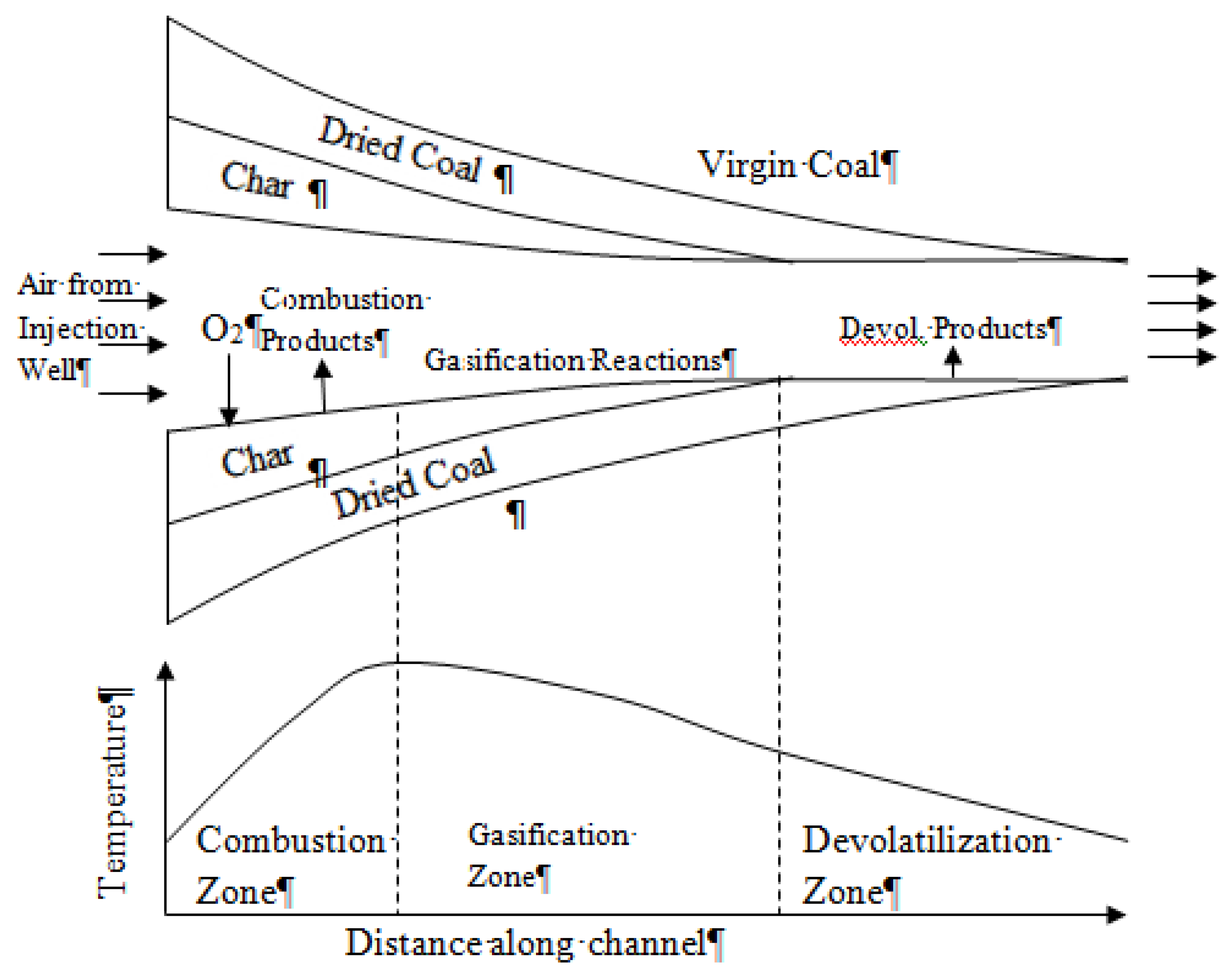
Some models have attempted to describe the UCG coal seam as a coal slab. These models describe the process by movement of various defined regions in a coal slab perpendicular to the flow of the injected blast gas. These regions usually include the gas film, ash layer, char region, dried coal, and virgin coal. The existence of different regions is due to the slow heating rate of the UCG. At a very high heating rate, there is a possibility of the coincidence of a drying front with a combustion front [
74]. The general framework of these models is shown in
Figure 36. Tsang [
74] was the first to use this approach considering the observation of the development of drying, pyrolysis, and gas-char reactions zones around the most permeable path in the coal seam. In addition, the profiles of temperature and saturation as well as the direction of heat and mass transfer exhibited from the pyrolysis experiment (
Figure 37) of a small coal block performed by Westmoreland and Forrester [
75] inspired him to consider necessary assumptions, such as the existence of a drying front, heat flux, and mass transfer direction,
etc., for this approach. In that experiment, a constant heat was applied to the coal surface and career gas was supplied along the length of the cylinder. Some researchers considered the virgin coal region as a wet zone due to the presence of water which is separated from the dry zone by the evaporation/drying front. The evaporation of water is assumed to take place entirely at the retreating drying front. Thus, the model following this approach must be a moving boundary value problem with phase change which is known as the “Stefan” problem. In this approach, as can be speculated from
Figure 36, there is an efflux of steam, devolatilized materials, and “self-gasification” products from the wall to the cavity, while there is a counter-current flux of heat towards the cavity wall. “Self-gasification” is considered as the reaction of the gases (steam and devolatilized gases) with hot char while they pass through it before flowing into the cavity. Because of the consideration of different layers, unlike other types of models, for each layer separate mass and energy balances are usually considered. As a result, the governing equations for mass and energy balances are of split boundary types. The mass flux is considered to be diffusion dominant.
Table 16 and
Table 17 represent a glimpse of a list of coal slab models discussed here with their essential features and reaction rate control mechanisms of the main reactions in the gasification process, respectively.
Figure 36.
Scheme of coal block models (modified from Perkins and Sahajwalla [
76]).
Figure 36.
Scheme of coal block models (modified from Perkins and Sahajwalla [
76]).
Figure 37.
Schematic diagram of temperature and saturation profile and heat and mass transfer in coal block (redrawn from Tsang [
74]).
Figure 37.
Schematic diagram of temperature and saturation profile and heat and mass transfer in coal block (redrawn from Tsang [
74]).
Table 16.
Some essential features of reported coal slab models.
Table 16.
Some essential features of reported coal slab models.
| Researchers | Dimension and Time Dependence | Heat Transfer | Mass Diffusion | Fluid Flow | Thermo Mechanical Failure | Water Influx | Heat Loss |
|---|
| Conduction | Convection | Radiation |
|---|
| Tsang [74] | 1D and T | √ | √ | √ | √ | | | √ | |
| Massaquoi and Riggs [77,78] | 1D and S | √ | √ | | | D | | | √ |
| Park and Edgar [79] | 1D and T | √ | √ | | | D | | | |
| Perkins and Sahajwalla [76,80] | 1D and PS | √ | √ | √ | √ | NS | √ | √ | |
Table 17.
Reaction rate control mechanisms of the main reactions in the gasification process.
Table 17.
Reaction rate control mechanisms of the main reactions in the gasification process.
| Researchers | Drying | Pyrolysis | Char Reaction | Water-Gas Shift Reaction | Gas Phase Reaction |
|---|
| C + O2 → CO2 | C + CO2 → 2CO | C + H2O → CO+ H2 | C + 2H2 → CH4 | CO + H2O↔ CO2+ H2 | CO + 0.5O2 → CO2 | H2 + 0.5O2 → H2O | CH4+2O2→ CO2+2H2O |
|---|
| Tsang [74] | H | P | | P | P | | K | | | |
| Massaquoi and Riggs [77,78] | H | P | | P | P | | E | I | I | |
| Park and Edgar [79] | H | P | D | P | P | | | I | I | |
| Perkins and Sahajwalla [75,80] | H | P | | P | P | P | E | | | I |
As stated earlier, Tsang [
74] was the pioneer of the approach and developed a 1D unsteady UCG model considering the two regions of a coal block: the wet zone, and dry zone. In the wet zone, heat conduction and liquid transfer are solved. It was assumed that all drying happens in one moving point (Stefan model). In this model, the movement of the drying front was described using the following equation:
where Δ
Hv is the heat of the evaporation of water,
is the location of the drying front.
This model neglected the effects of steam convection and assumed that the drying process was dominated by conduction. In the wet zone, the liquid diffusion was considered as a function of saturation; however, for the dry zone, multicomponent diffusion was calculated using viscous flow. In the dry region, the pseudo-steady-state assumption was adopted to solve mass balance, heat transfer, and gas flux. Pyrolysis reactions were modeled as simultaneous independent reactions with kinetic parameters obtained from the works of Campbell [
49]. Porosity and permeability were set to change with the extent of the reactions with correlations obtained from oil well acidization. This model neglected the combustion and provided the heat by setting a high temperature at the boundary. The experimental results of Forrester [
81] were used for model validation. The calculated drying front locations with time were found to be in good agreement with the experimental data (
Figure 38). However, the effect of the heating rate on the location of the drying front shows that a higher surface heating rate causes a shallower penetration of the drying front into the coal block (
Figure 39). This observation indicates the possibility of the coincidence of the drying front with the combustion front at a very high heating rate. Finally, it was concluded from the model that drying cannot be neglected in the UCG model as it is a factor that dominates the heat transfer rate.
Figure 38.
The location of the drying front as a function of time [
74].
Figure 38.
The location of the drying front as a function of time [
74].
Figure 39.
Effect of the heating rate on the location of the drying front [
74].
Figure 39.
Effect of the heating rate on the location of the drying front [
74].
Massaquoi and Riggs [
77,
78] extended Tsang’s 1D model by including the combustion of char and volatiles at the boundary while solving for a steady-state case. Beside the zones shown in
Figure 36, they included another zone of bulk gas that is composed of water vapor, CO
2, O
2, and some inert gases outside the gas film. The developed model was used to describe the simultaneous combustion and drying of a wet Texas lignite coal. The flow of gases in the porous dry coal was modeled by Darcy’s law and heat transfer was considered by both conduction and convection. However, in the wet zone, only conduction was considered for heat transfer. Radiation heat transfer was also considered between the edge of the ash and the bulk gas. Because of the drop in the total pressure across the dry coal and the high permeability of pyrolyzed coal, mass flux was assumed to happen mainly by viscous flow. Multi-component diffusion was assumed to occur at different zones. They considered almost all the reactions listed in
Table 1 except for methanation. Following the approach of Tsang [
74], pyrolysis reactions were modeled as simultaneous independent reactions with kinetic parameters obtained from the works of Campbell [
49]. Because of steady-state assumptions, all the governing equations were written in ordinary differential equations in terms of the moving coordinates. The cavity wall and the drying front movements were considered to have same velocity. In their model, two different cases for combustion were assumed: (i) homogeneous char combustion with the flame located at the ash; and (ii) heterogeneous char combustion with the flame located at the coal surface, and finally a criterion was defined for the transition from heterogeneous to homogenous combustion. For the case of Wyodak subbituminous coal, their result indicated that the criteria principally depend on the conditions of bulk oxygen concentration, bulk gas temperature, coal surface temperature, and coal burning rate. However, different solutions can be obtained at different conditions. For example, as seen in
Figure 40, it is found that, for a given bulk gas temperature, there is a limiting bulk oxygen concentration and an oxygen concentration above the limiting bulk; for a fixed oxygen concentration and bulk gas temperature there are two possible solutions (
Figure 40): one with the flame at the coal face (at a lower surface temperature) and another with the flame in the ash (at a higher surface temperature). However, heterogeneous combustion was considered unstable due to the decrease of the coal face temperature with the increasing bulk gas temperature for a constant oxygen concentration. In contrast, homogenous combustion was considered stable because of the experimental observation reported in the literature [
82,
83,
84]. They also indicated a maximum value of the bulk gas temperature above which the flame is always away from the coal surface.
Figure 40.
Effect of bulk gas temperature of the combustion of wet Wyodak coal [
78].
Figure 40.
Effect of bulk gas temperature of the combustion of wet Wyodak coal [
78].
In addition, they have concluded that the burn rate would be nearly linear with the increase in the concentration of oxygen when the flame front is located in the char face, and the burn rate increases when the flame is located in the gas film (
Figure 40). In their model, the effect of the ash layer thickness, coal moisture content, and film transport coefficients were also discussed. A higher film mass transfer coefficient and a lower moisture content and ash layer are observed to shift the transition line towards higher coal surface temperatures corresponding to the higher burning rate for a constant bulk oxygen concentration. For the homogeneous combustion model, the performance of the model was in good agreement with the experimental data [
83,
84].
Park and Edgar [
79] developed an unsteady 1D model with a moving burning front based on the work of Massaquoi and Riggs [
77,
78] to describe lateral cavity growth in UCG. However, unlike the assumption of Massaquoi and Riggs [
77,
78], they did not consider having the same velocity for the cavity wall and drying front during the early stage. Beside char gasification, they included coal shrinkage due to drying and pyrolysis, as well as the “self-gasification” of drying and pyrolyzed products (steam and CO
2) in the region between the cavity wall and the drying front in order to consider the additional movement of the cavity wall. The cavity wall movement was determined by the rate of the removal of coal by chemical reactions and the physical movement of the cavity wall due to the shrinkage of the coal. In their simulation, an increase of the cavity growth was noticed during the transient period due to the shrinkage of the coal; however, the cavity growth with and without considering the shrinkage eventually merged into one rate when the steady state was reached (
Figure 41). However, they suggested that the movement of the cavity wall due to shrinkage is only important in lab-scale processes and can be neglected in larger-scale processes because of the long timescales in which the transient period is negligible compared to the steady-state period. Their results indicate that cavity growth is controlled by the rate of oxygen transfer to the cavity wall, when the flame is located at the char surface. If the flame is separated from the cavity wall, CO
2 and steam gasification determine the cavity growth rate. The moisture content in coal was found to be a complex parameter for cavity growth. Although the surface temperature decreased with increasing moisture content, the higher moisture content indicated a higher cavity growth at a high coal surface temperature (above 1000 °C). This observation implies that the availability of water in the coal, rather than the reaction temperature, controls the steam gasification reaction rate. They validated their results with the experimental data of lateral cavity growth from a Texas lignite core combustion performed by Poon
et al. [
85]. From the models discussed above [
77,
78,
79], it can be speculated that under oxidizing conditions, the cavity growth rates are controlled by mass transfer.
Figure 41.
Effect of the shrinkage on the cavity growth rate [
79].
Figure 41.
Effect of the shrinkage on the cavity growth rate [
79].
Perkins and Sahajwalla [
76,
80] also developed a 1D transient coal block model with an extension of Tsang’s study [
74] by including multicomponent diffusion and the random pore model to account for changes of heterogeneous reaction rates with conversion. For multicomponent diffusion, Stefan-Maxwell equations and the bi-dispersed dusty gas model were used for the gas film and dried coal matrix, respectively. Because of experimental evidence (
Figure 42) of different sizes of pore distribution in the porous structure of coal, a bimodal porous structure (macropores and micropores) was considered where the macropores act as the major conduits for species flow and the micropores act as the dominant region for gasification reactions.
Figure 42.
Pore structure of raw American coals on dry and ash-free basis [
70].
Figure 42.
Pore structure of raw American coals on dry and ash-free basis [
70].
They have proposed that cavity growth occurs at reducing conditions, therefore only heterogeneous gasification reactions are solved, and required heat was provided by defining a constant temperature at the char surface. The char surface was allowed to participate in radiation heat exchange with its surroundings. For pyrolysis, they followed the work of Tsang [
74]. The movements of the drying front and char front were assumed to be equal under pseudo-steady-state conditions. They assumed that solid and gas phases are in thermal equilibrium and bulk gas has a fixed composition that is representative of the product gas. In their first paper [
80], they validated their model with the experimental data obtained by Forrester [
81]. The drying front location as a function of time was in good agreement after using a scaling factor of 1.2 for thermal conductivity (
Figure 43). The temperature profile through the block at different surface temperatures also agreed well with the experimental data. However, when the cavity growth rates as a function of gas temperature for two different bulk gas compositions were compared, no significant difference was observed (
Figure 44).
Figure 43.
Drying front location as a function of time for cylindrical coal block heating experiments [
80].
Figure 43.
Drying front location as a function of time for cylindrical coal block heating experiments [
80].
Figure 44.
Cavity growth rate, as a function of gas temperature, for two different bulk gas compositions [
80].
Figure 44.
Cavity growth rate, as a function of gas temperature, for two different bulk gas compositions [
80].
In a later paper [
76], they extended their work by including the ash layer and water influx and investigated the effect of various parameters and operating conditions (e.g., temperature, pressure, water influx, gas composition) on the process performance and cavity growth rate. In order to compare the relative effect on cavity growth due to operating conditions and coal properties, they explored the sensitivity of the cavity growth rate (
vcv) to changes in parameters (
pr) using the following finite difference formula:
where
s(pr) is the sensitivity of the parameter,
pr° is the base value of the parameter, and Δ
pr is a perturbation to the value of the parameter.
A ranking was established according to the sensitivity of the parameters to the cavity growth rate. A positive value was considered as an increase in
vcv, while a negative value was considered in reverse order.
Table 18 and
Table 19 show the sensitivity of the cavity growth rate to perturbation in operating conditions and coal properties around the base values,
p°. Since the summation of the composition of proximate analysis is equal to one, changing any one of these parameters was followed by adjusting the other parameters in order to maintain the constraint of the summation of one.
Table 18.
Sensitivity of the cavity growth rate to changes in operating conditions [
76].
Table 18.
Sensitivity of the cavity growth rate to changes in operating conditions [76].
| Parameter | p° | Δp/p° = 10−3 | Δp/p° = 10−2 | Rank |
|---|
| Bulk gas temperature, K | 1.5 × 10³ | 5.276 | 5.276 | 1 |
| Water mass flux, kg/m2·s | 1.0 × 10⁻³ | −0.114 | −0.115 | 2 |
| Mole fraction of steam in bulk gas | 2.0 × 10⁻¹ | 0.066 | 0.071 | 3 |
| Ambient pressure, Pa | 1.5 × 10⁶ | 0.079 | 0.067 | 4 |
| Mole fraction of CO2 in bulk gas | 1.2 × 10⁻¹ | −0.009 | −0.009 | 5 |
| Mole fraction of H2 in bulk gas | 1.6 × 10⁻¹ | 0.008 | 0.008 | 6 |
| Heating rate, K/s | 1.0 × 10⁻² | 0.006 | 0.007 | 7 |
| Mole fraction of CO in bulk gas | 8.0 × 10⁻² | 0.005 | 0.005 | 8 |
Table 19.
Sensitivity of the cavity growth rate to changes in coal properties [
76].
Table 19.
Sensitivity of the cavity growth rate to changes in coal properties [76].
| Parameter | p° | Δp/p° = 10−3 | Δp/p° = 10−2 | Rank |
|---|
| Critical conversion of carbon at which the coal spalls | 9.50 × 10⁻¹ | −3.719 | −3.741 | 1 |
| Mass fraction of fixed carbon from proximate analysis | 3.35 × 10⁻¹ | −1.359 | −1.370 | 2 |
| Solid material density (kg/m3) | 1.47 × 10³ | −0.913 | −0.925 | 3 |
| Mass fraction of ash from proximate analysis | 2.40 × 10⁻¹ | 0.714 | 0.728 | 4 |
| Ash layer thickness (m) | 5.00 × 10⁻³ | −0.689 | −0.703 | 5 |
| Mass fraction of volatile matter from proximate analysis | 3.00 × 10⁻¹ | 0.589 | 0.576 | 6 |
| Mass fraction of moisture from proximate analysis | 1.25 × 10⁻¹ | 0.344 | 0.331 | 7 |
| Emissivity of ash (for radiation) | 8.50 × 10⁻¹ | 0.114 | 0.127 | 8 |
| Initial specific surface area (m2/m3) | 1.23 × 10⁷ | 0.105 | 0.105 | 9 |
Results of their parametric study indicate that temperature of the coal surface, water influx, and coal composition have the highest impact on the cavity growth rate. Decreasing fixed carbon was found to increase the cavity growth rate. This implies that the cavity growth rate is more for low-rank coal due to the smaller fraction of fixed carbon in the proximate analysis. Perkins and Sahajwalla [
76] graphically demonstrated the variation of cavity growth due to the variation of different parameters through their modeling. In addition, they incorporated the coal spalling model by changing the value of the critical conversion,
Xcritical. Due to lack of information on coal spalling, they considered the critical conversion of fixed carbon as an indicator of coal spalling by assuming a level of carbon conversion at which some fixed carbon and volatile matter are unconverted and detach from the coal block due to mechanical stress and breakage. Critical conversion was found sensitive to the bulk gas temperature, molar flux of product gas, and water influx.
Finally, they compared the estimated cavity growth rate from their simulation with six different field trials (Hanna I, Pricetown, Large Block Test No. 5 (LBK-5), Partial Seam CRIP (PSC), Rocky Mountain I (RM I), and El Tremedal) using the available operating conditions and coal properties of those field trials and obtained a good agreement with the data from the field trials (
Figure 45) despite some uncertainty of the field data. Although they conducted a detailed study of the coal block model, they did not consider char combustion and other gas phase reactions (except the water-gas shift reaction) which are strong functions of the temperature. Rather, the assumption of a constant temperature and fixed gas composition at the boundary limits the applicability of the model to field trials.
Figure 45.
Comparison of estimated cavity growth rates from six UCG field trials with model simulations [
80].
Figure 45.
Comparison of estimated cavity growth rates from six UCG field trials with model simulations [
80].
The special feature of the coal slab model is the tracking of the drying and combustion front movement. This model can successfully demonstrate the drying and devolatilization behaviour of large coal particles; however, this model is yet to be validated using UCG field trial data. Due to the assumption of semi-infinite coal slab, it can be speculate that this model is only good for a thick coal layer. All the models developed thus far by considering the coal slab are one-dimensional (1D). As a result, information on cavity shape cannot be obtained from these models.


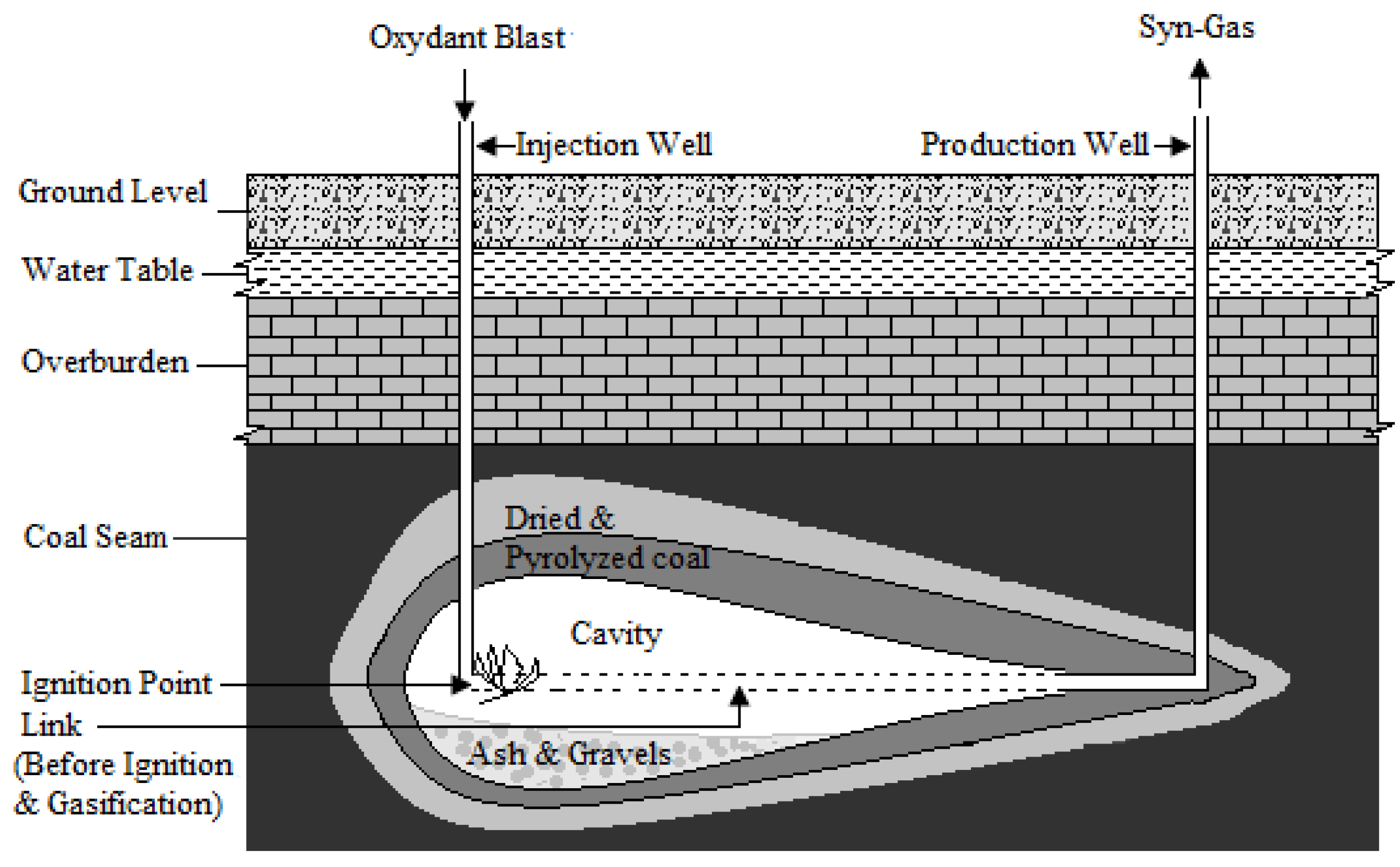
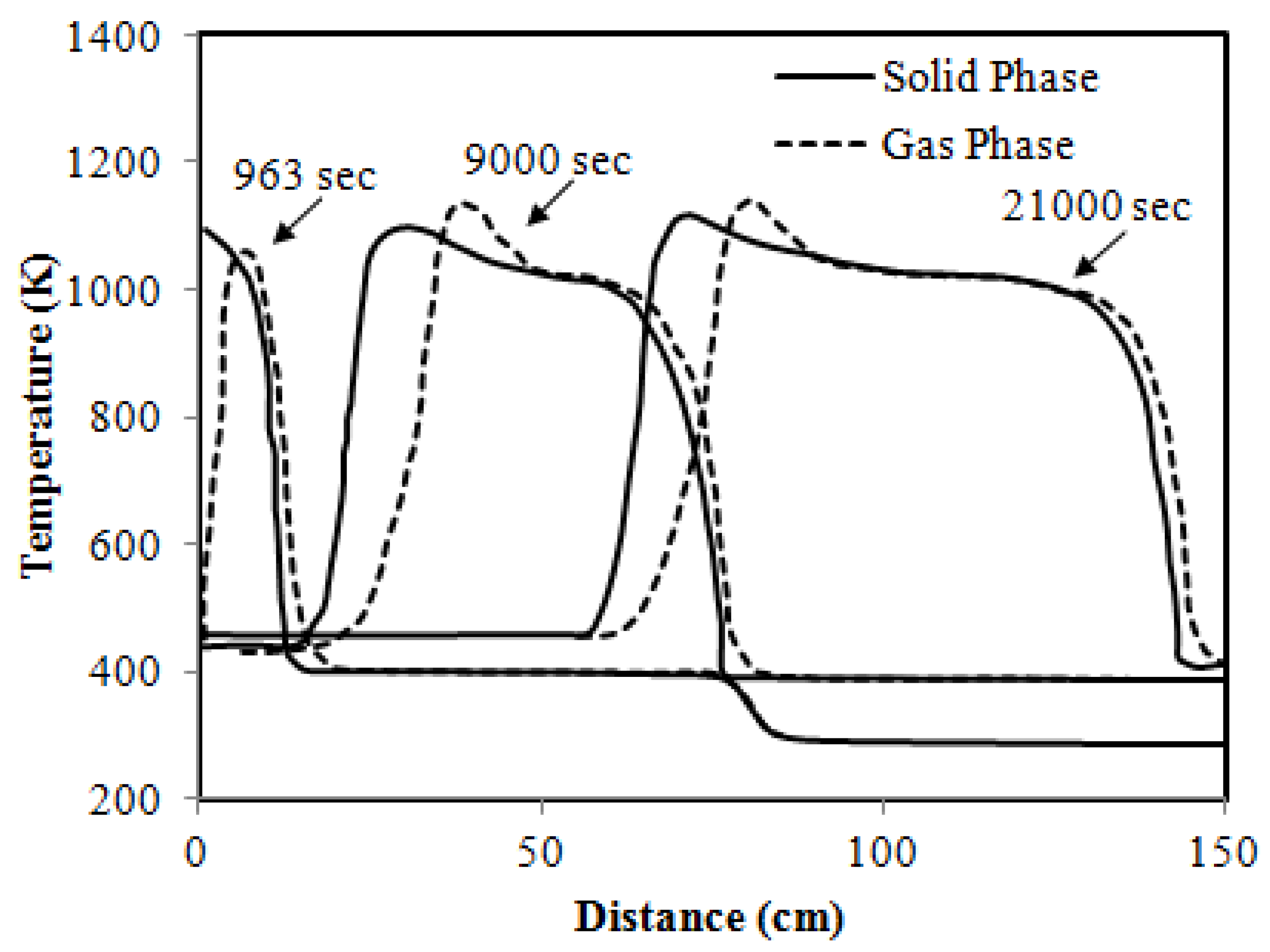
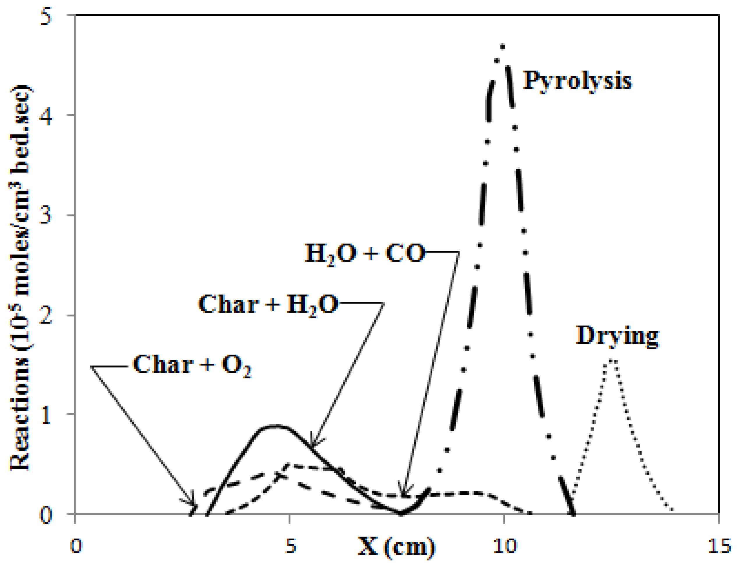
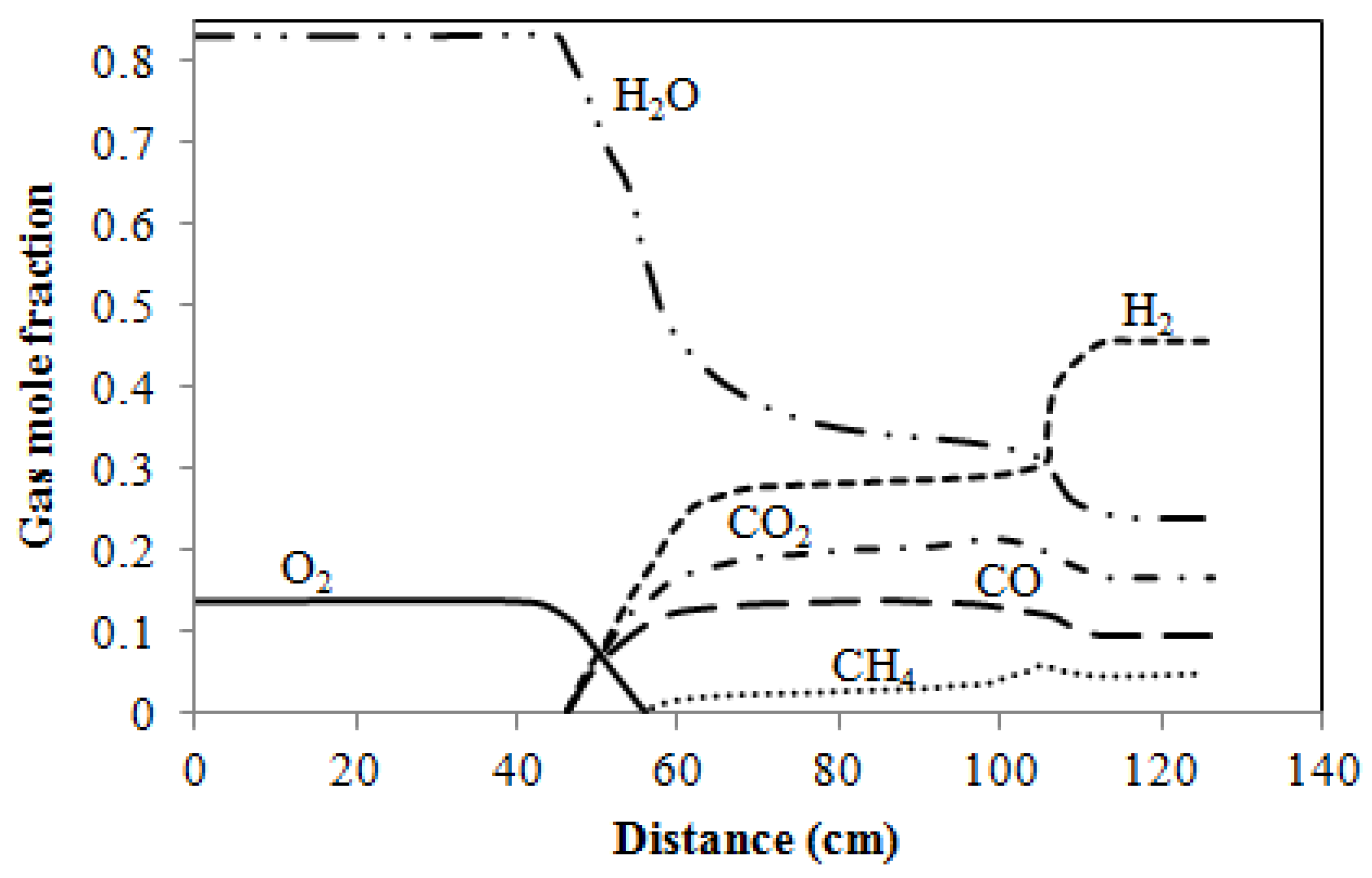
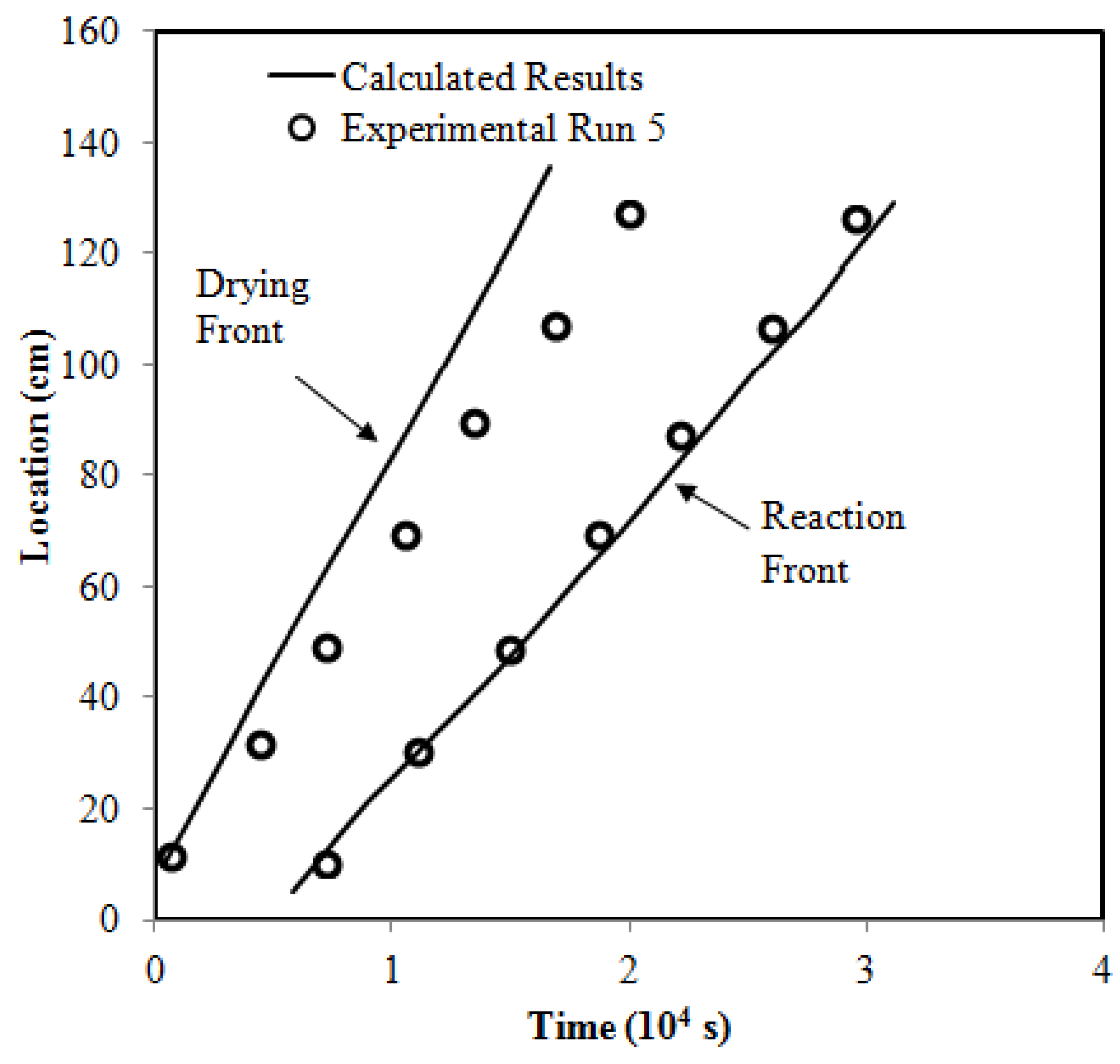
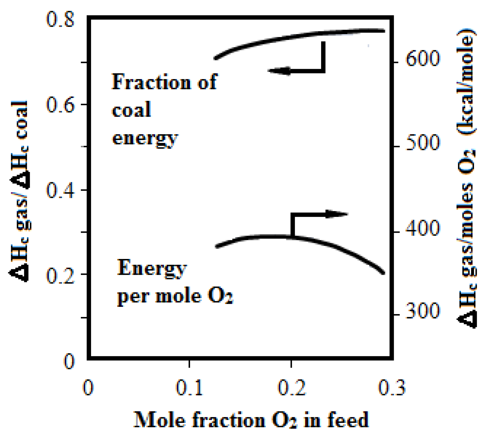
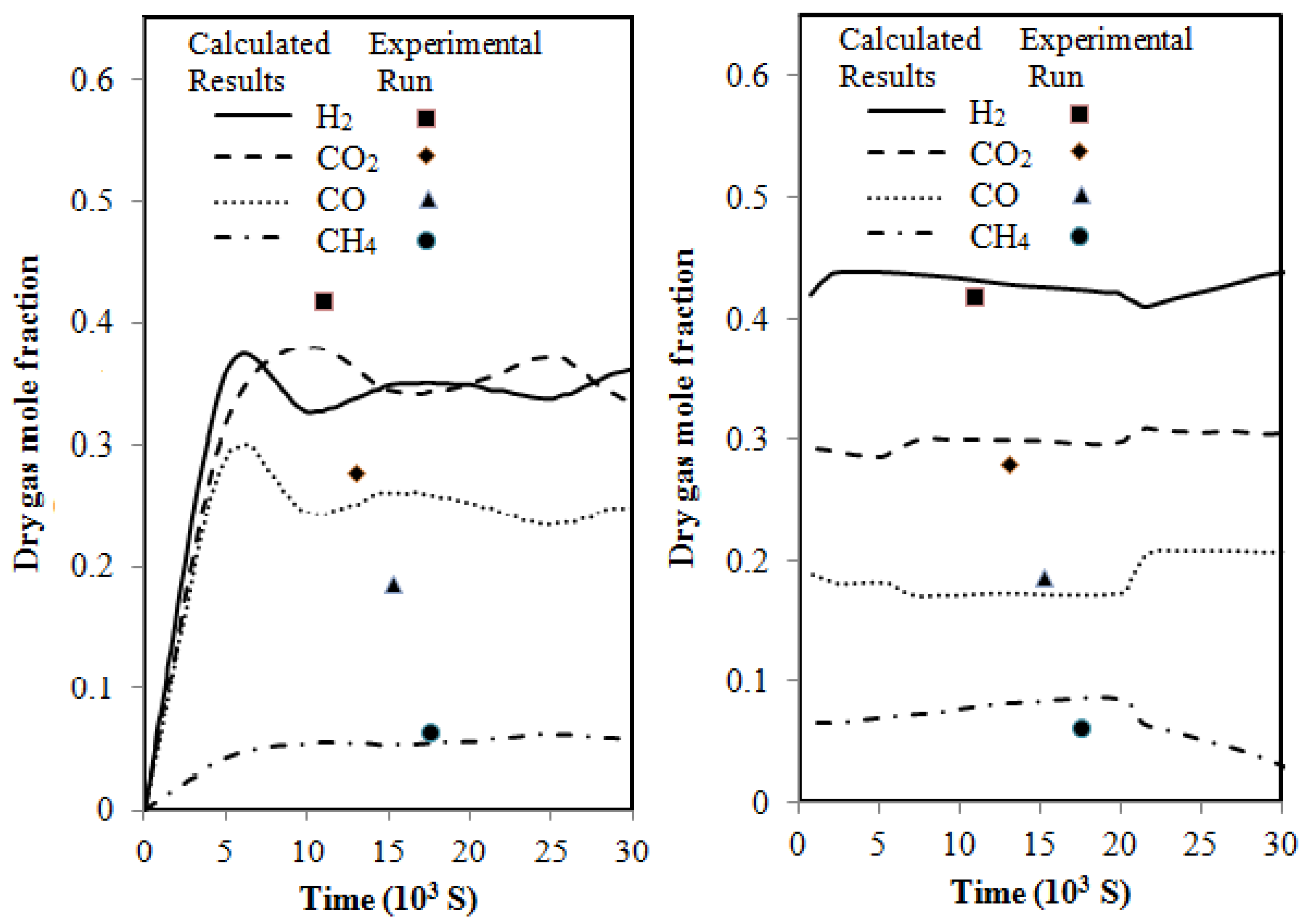
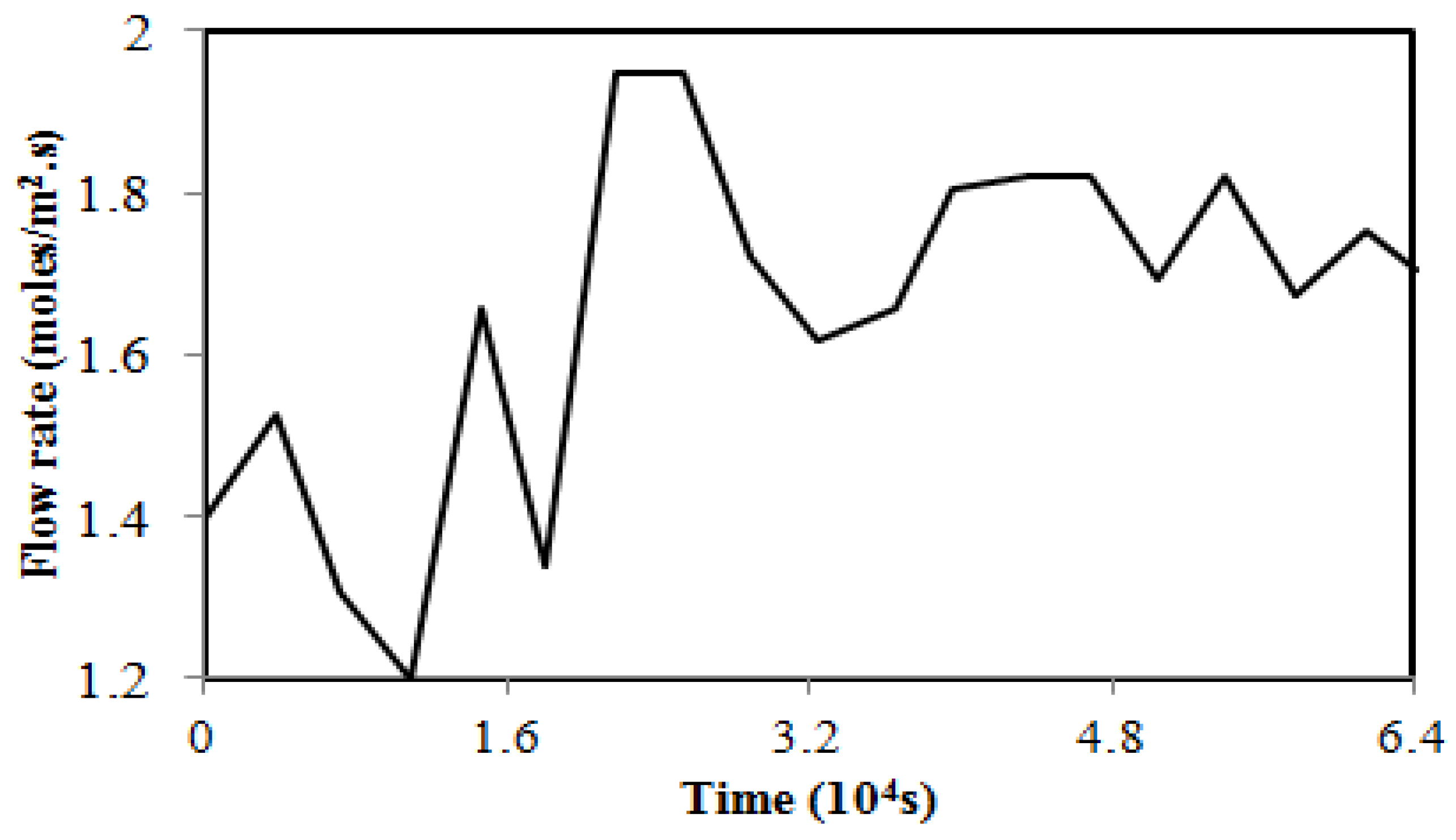
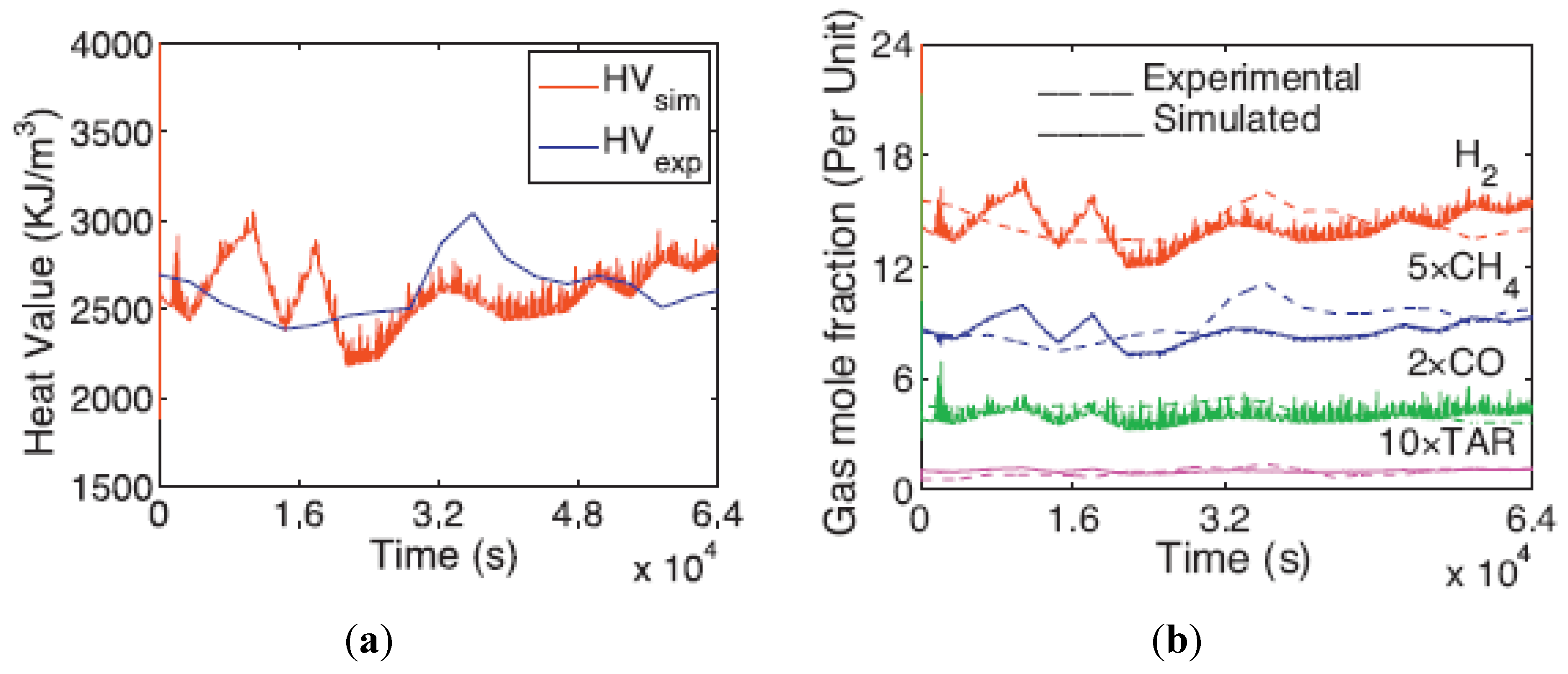
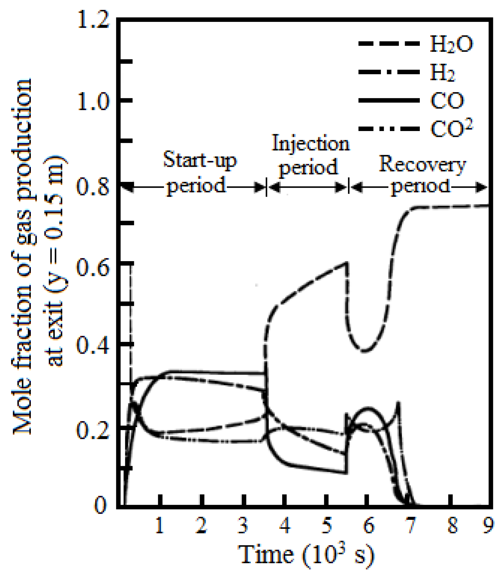
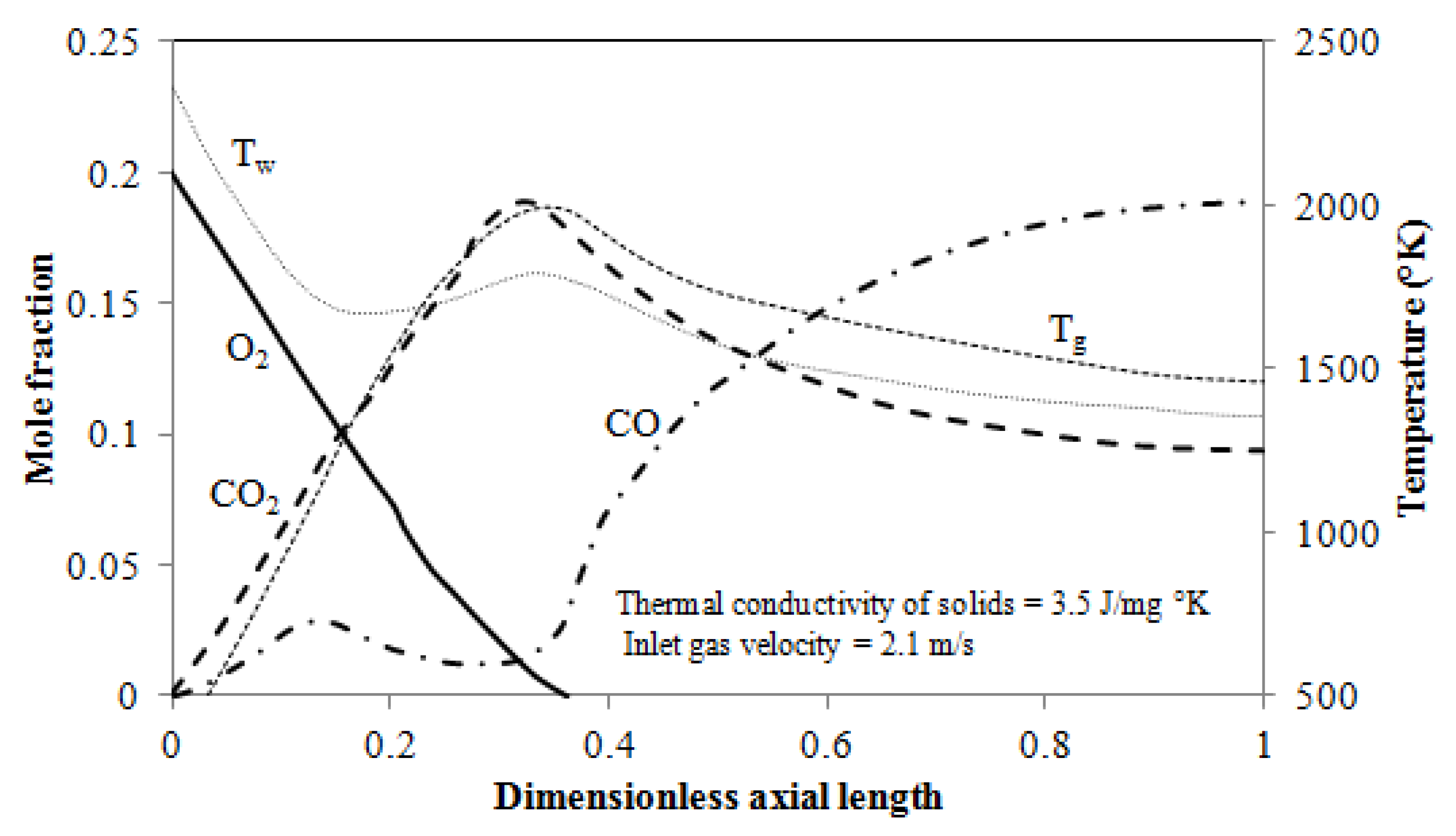
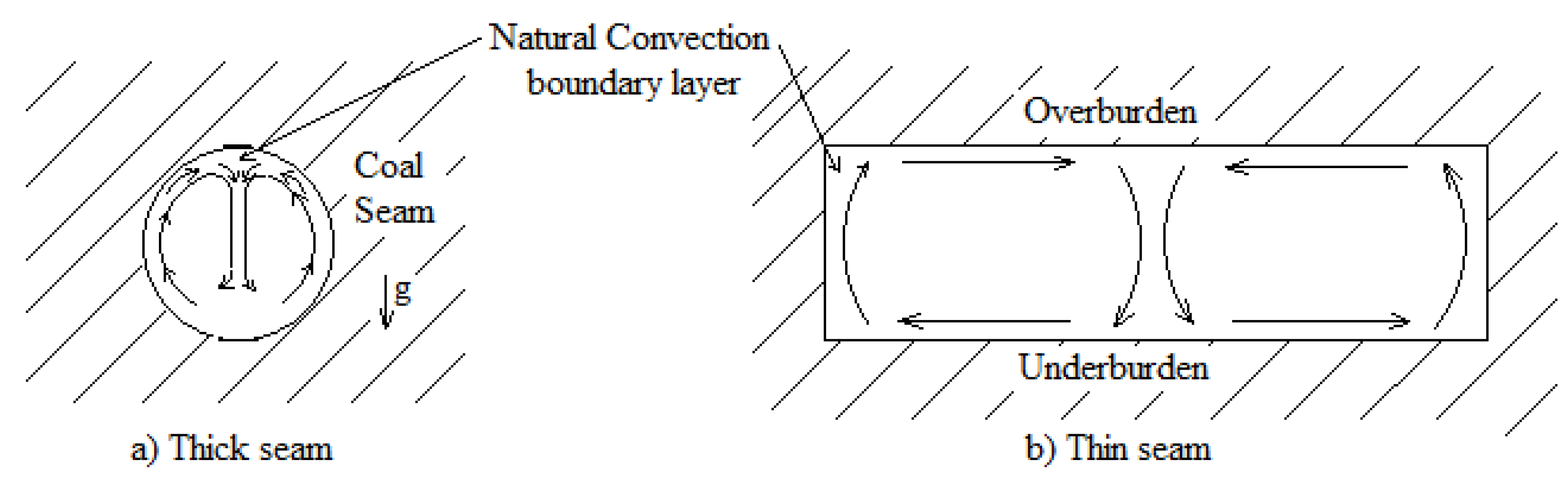
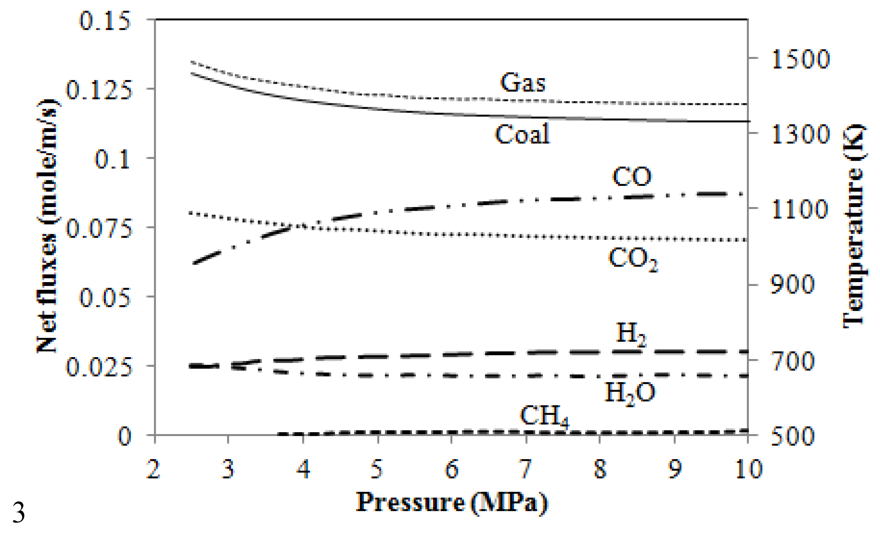
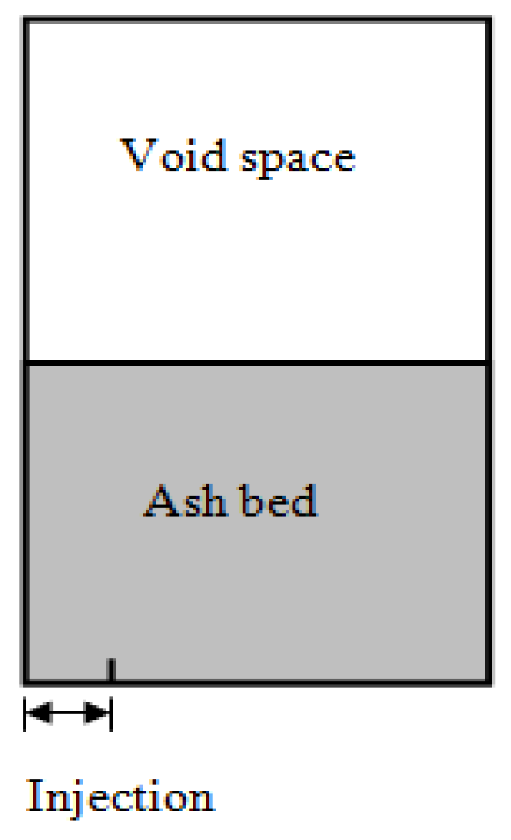
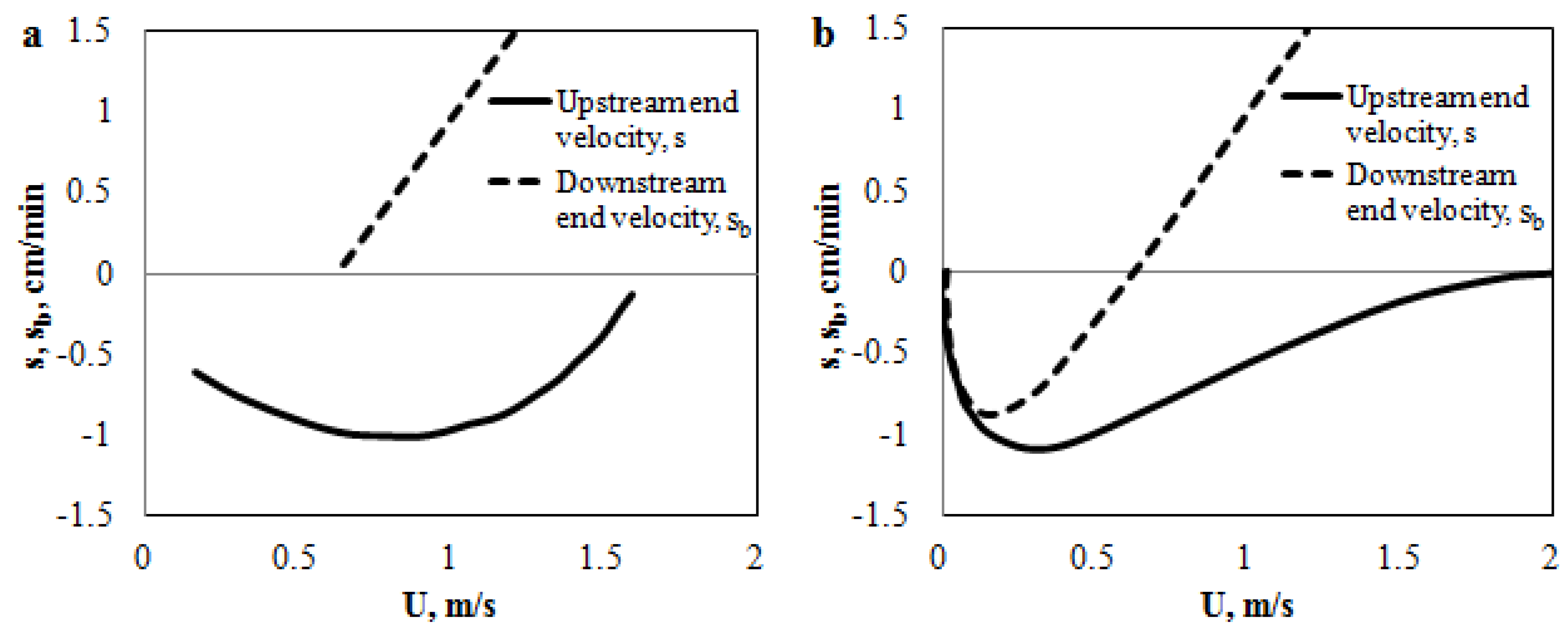
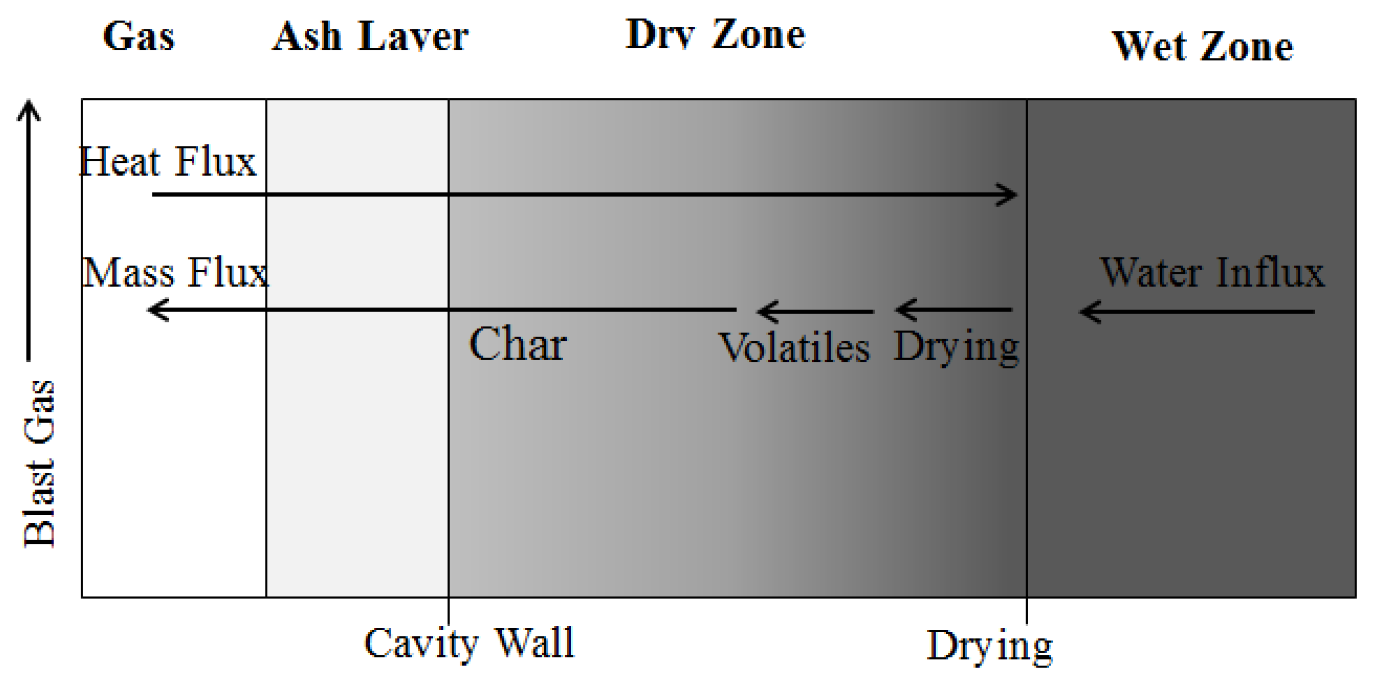
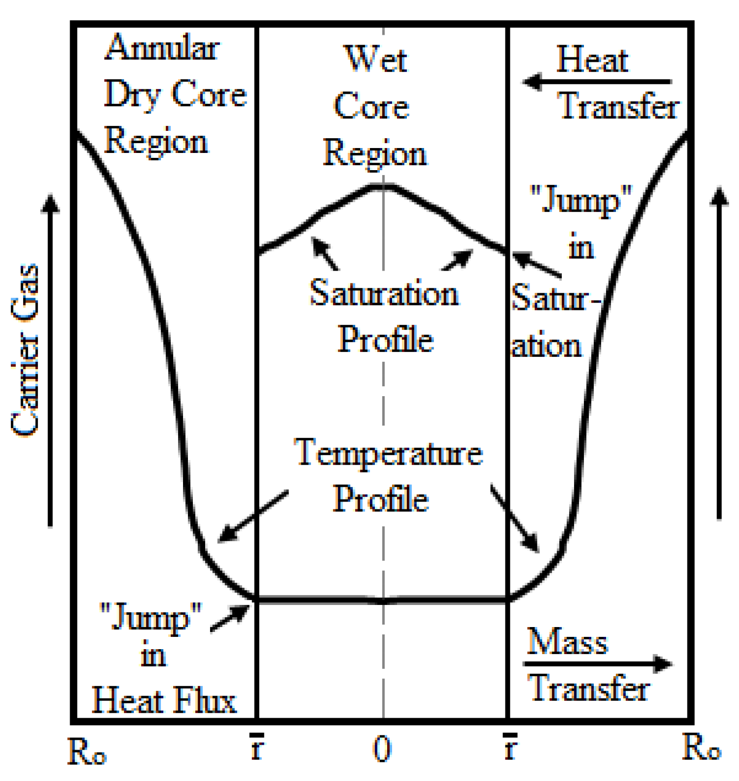
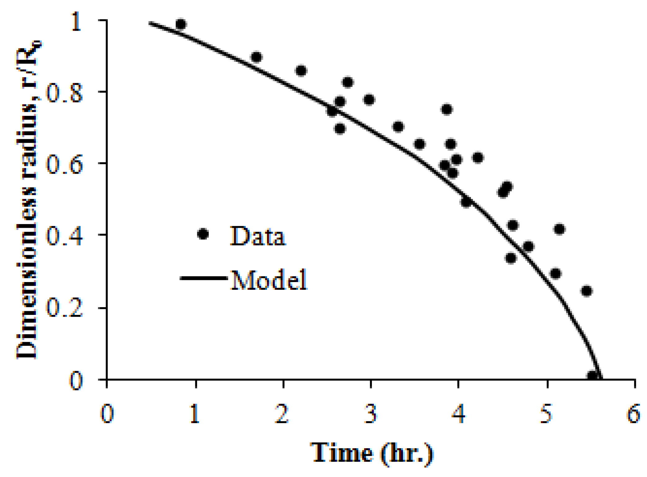
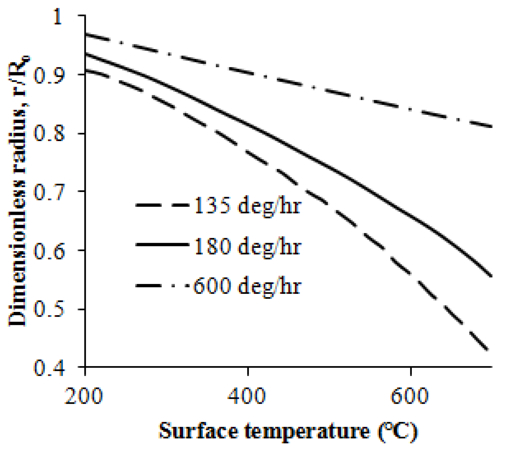
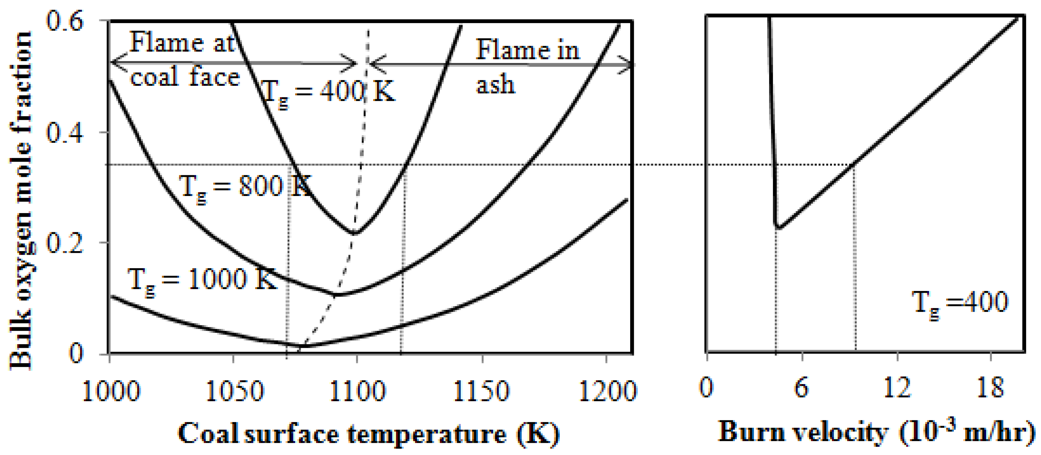
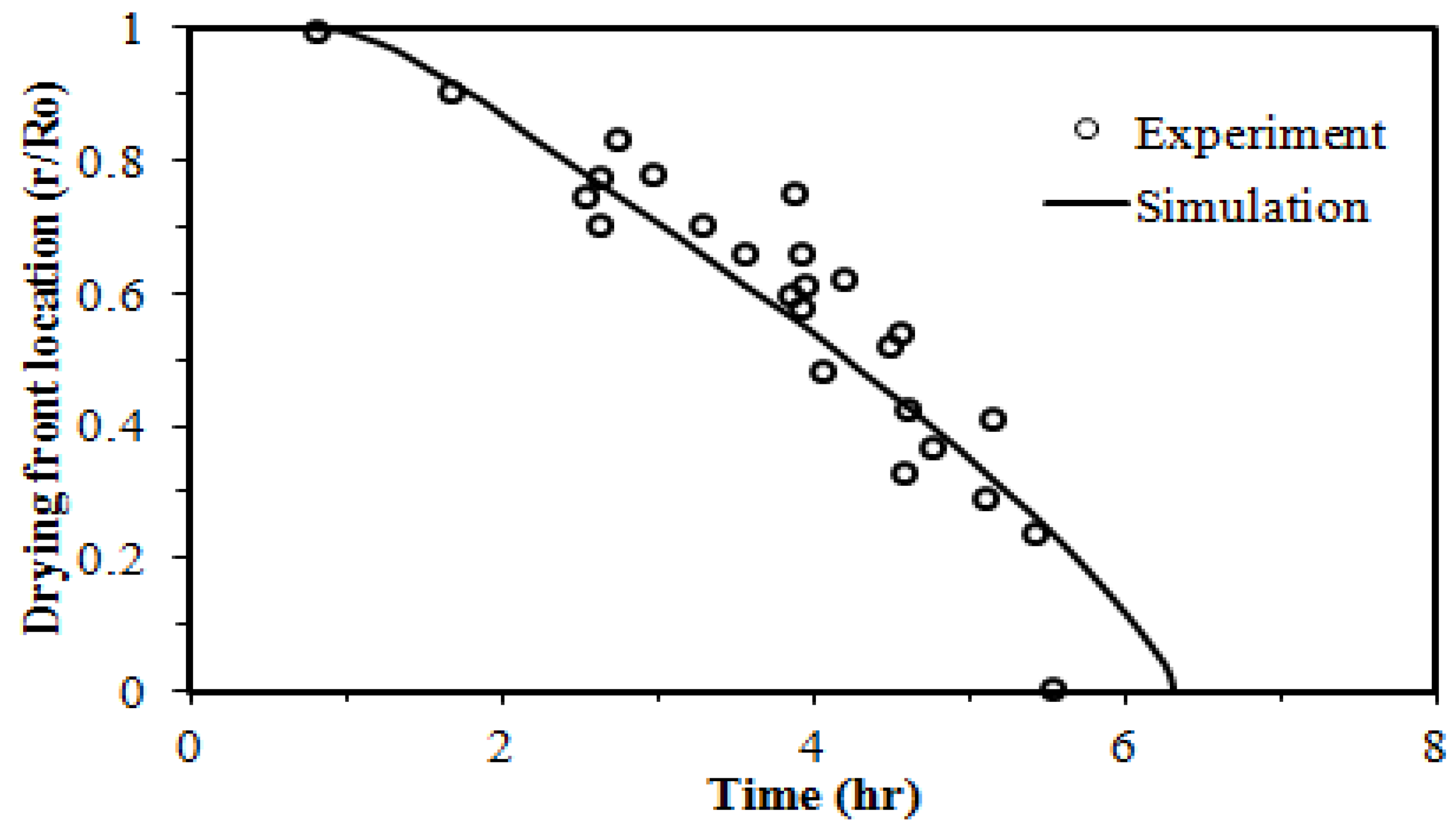
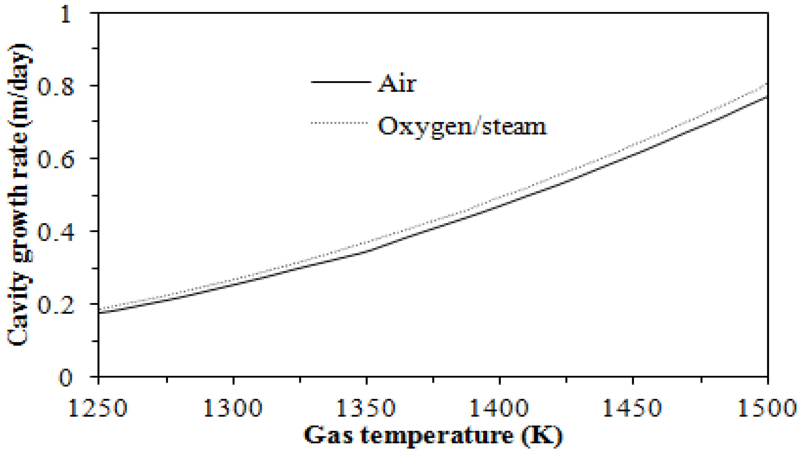
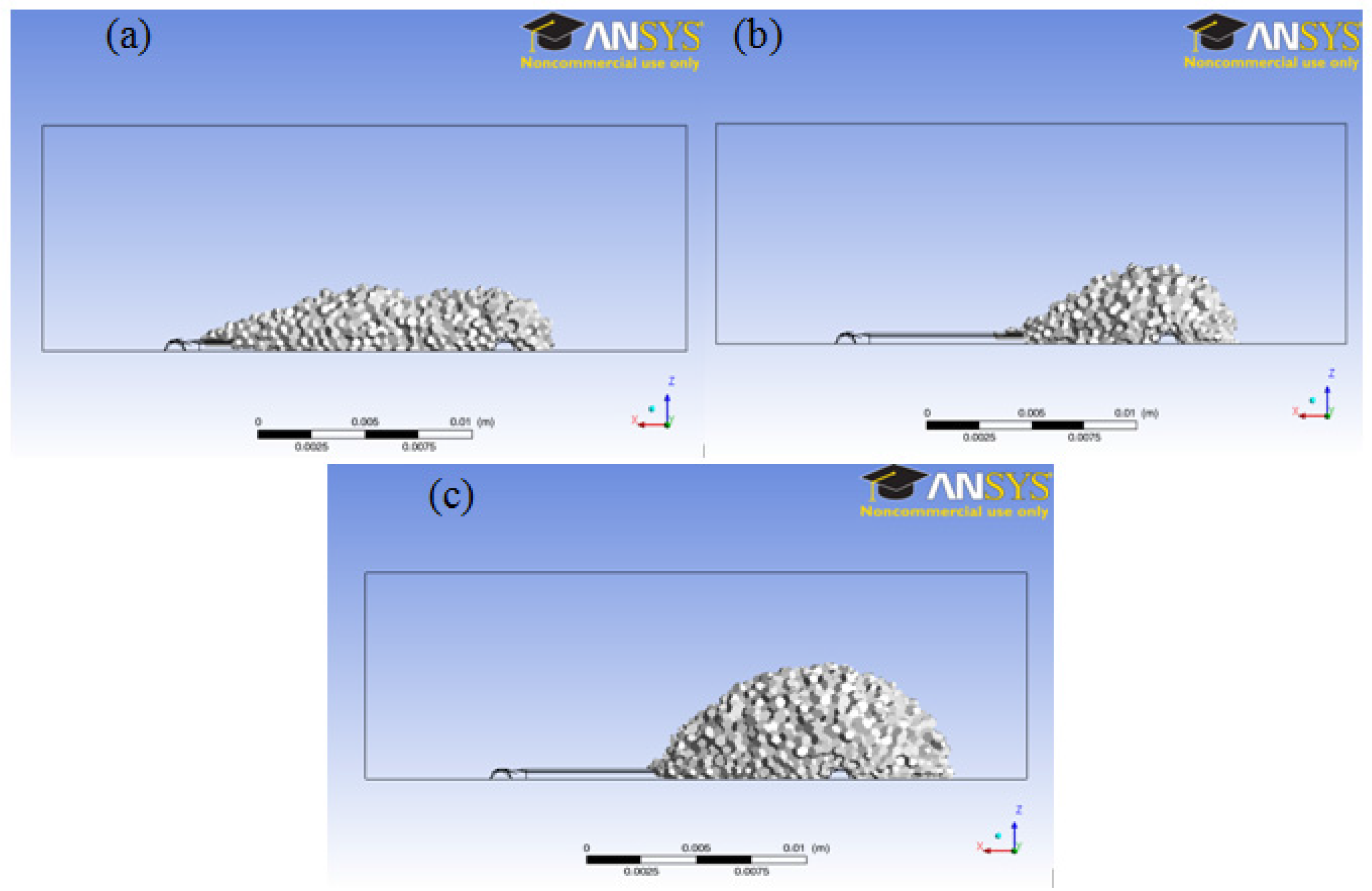
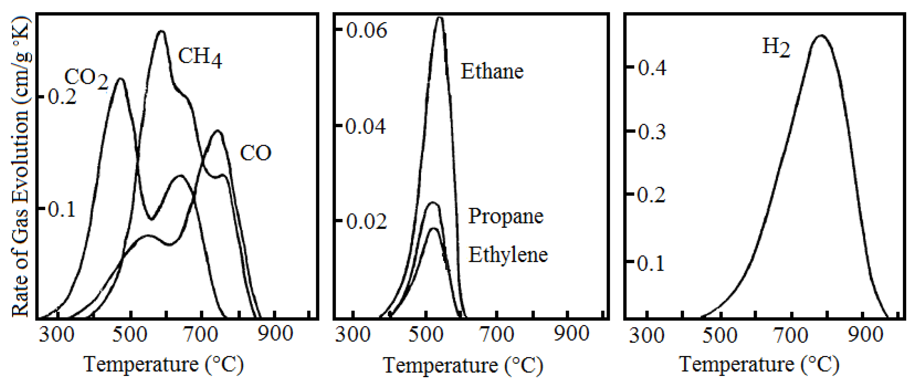
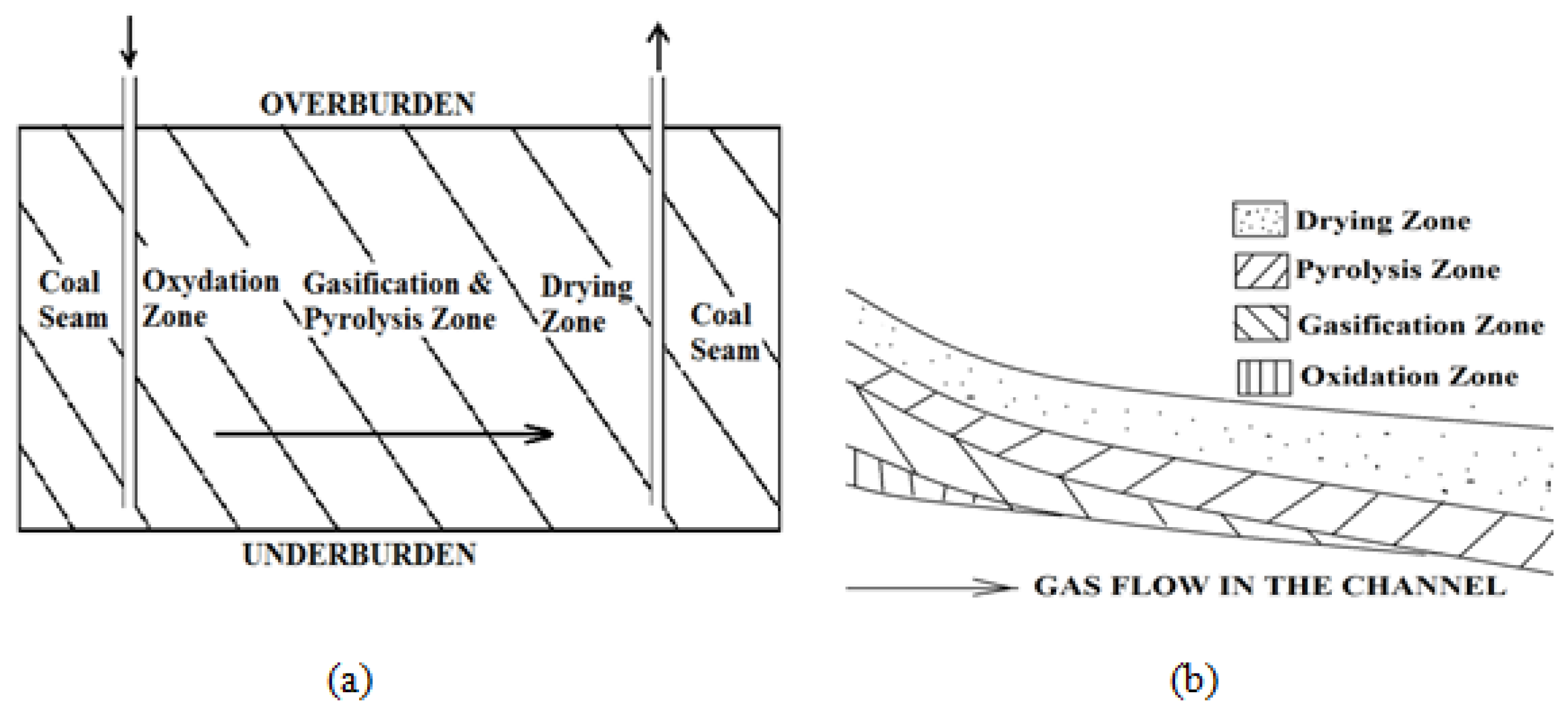