A First-Order Study of Reduced Energy Consumption via Increased Thermal Capacitance with Thermal Storage Management in a Micro-Building

Abstract

This study uses a first-order approximation of a micro-building to investigate the major factors determining how increased thermal capacitance (ITC) with thermal storage management (TSM) can reduce energy consumption in locations with relatively mild weather conditions such as the southeastern part of the United States of America. In this study, ITC is achieved through water circulation between a large storage tank and pipes embedded within the building envelope. Although ITC results in a larger dominant time constant for the thermal response of a building, an adaptive allocation and control of the added capacitance through TSM significantly improves the benefits of the extra capacitance. This paper compares two first-order models for a micro-building: a reference case model with a single lumped thermal capacitance associated with the building, and another model, with the building’s capacitance plus the capacitance of the water system. Results showed that the ITC/TSM system reduced the cost of conditioning the building by reducing the operating time of both the cooling and the heating systems. May through September, the air conditioning operating time was reduced by an average of 70%, and October through April, the operation of the heating system was reduced by an average of 25%.

1. Introduction

Increased thermal capacitance has been a subject of research for many decades [1,2,3,4]. Researchers such as Madhumathi et al. [5] and Zhu et al. [6] investigated the use of phase change materials to improve energy consumption due to climate control in dwellings located in hot environments. Similarly, Tan et al. [7] and Shi et al. [8] investigated the use of phase change coatings for heat management. In the early 60s, increased capacitance was part of a solar building plan through the study of geodesic domes [9,10]. However, the use of thermal management was not combined with thermal capacitance. A drawback of using a fixed thermal capacitance, i.e., without thermal management, is that the increased time constant associated with the added thermal capacitance can be detrimental to the operation of an air conditioning (AC)/heating system in situations when the temperature of the fixed capacitance remains above or below the thermal comfort specifications for a prolonged period of time.

Thermal energy storage is typically classified into passive and active operation. Passive methods allow free convection, conduction, and other natural heat transfer modes, whereas active methods uses forced convection as the main mode of heat transfer [1]. Passive methods for controlling the thermal conditions of a building are beneficial for multiple reasons. Passive designs can take advantage of building properties to avoid wasting electricity or fossil fuel, and thus can reduce operating costs for a building [1]. More important, however, is the environmental impact that passive methods have by reducing dependence on electricity and fossil fuel. Many government entities are providing tax credits to reduce the carbon footprints of residential homes. As an example, consider California’s Zero Net Energy initiative, whose goal is that all new residential buildings produce the same amount of energy consumed per year [11]. Passive methods such as earth coupling, where buildings are constructed to benefit from consistent temperatures below the surface of the earth [2], can have a negative influence on building operating costs. This is because of the permanent additional capacitance during seasons when minimal capacitance is optimal. In this paper, simulations for a primarily passive method are considered. A fixed additional capacitance could be considered a solely passive method, but the proposed method is semi-passive in that it uses water flowing through pipes in the walls. It has been found that a relatively small mass flow rate flowing through pipes embedded in the walls provides modest energy savings in achieving thermal comfort [3].

Using transient simulations for a one-room enclosure incorporating an increased thermal capacitance (ITC) system, Carpenter et al. [3] determined that the most beneficial placement of the additional capacitance is the ceiling, i.e., to circulate water from a tank through piping embedded in the ceiling. However, the energy savings due to their ITC methodology were rather modest, not taking full advantage of the weather conditions. In order to improve on the work of Carpenter et al. [3], a more advanced thermal management system (TSM) is proposed in this paper. The proposed ITC/TSM discussed in this paper takes advantage of daily maximum or minimum ambient temperatures to control the temperature of the water used in the ITC. Daily maximum temperatures during the winter months are used to heat the water and daily minimum temperatures during the summer are used to cool the water. The idea is to operate the ITC in such a way that the additional capacitance can be disengaged from the building envelope when the operation is unfavorable to the energy consumption of the building. Furthermore, an additional heat exchanger to the environment is incorporated into the water loop so as to help improve the temperature of the water for further energy savings.

Micro homes are very small houses, typically less than 18.56 m² (200 ft²) and can be as small as 9.29 m² (100 ft²) [12,13]. The building selected for this study is comparable to such micro homes. Although the size of the building in this study is small in comparison with standard residential dwellings, it will serve as a good start to establish the merit of the ITC/TSM concept, as well as to provide results that can be readily tested by constructing a micro home with ITC/TSM. Once the results for the ITC/TCM are established for a micro home, and lessons are learned regarding implementation of the ITC/TCM, this research will be adapted and extended to residential dwellings of standard sizes. Furthermore, a micro home lends itself well to first-order transient modeling, using a simple thermal lumped capacitor/resistance model. This will help lead to a better understanding of how to design the TSM without dwelling into the many complexities of a comprehensive and exhaustive building simulation. Although a first-order thermal model will not account for all features of a standard residential building, first-order transient approximations are commonly used to provide improved assessment of the dynamic performance of a building over pure static models [4], and are often used to understand the main aspects governing the response of a system that are not necessarily apparent from detailed and complex computational models. In addition to the above, simple models are much more suitable for real time implementation in actual control systems. As mentioned above, the models developed in this study use lumped resistance/capacitance (RC) thermal circuit elements. Two simple circuits, a reference circuit, and an ITC/TSM circuit were simulated on a month-by-month basis for an entire year and the temperatures for the building and the embedded envelope were calculated every 20 s. The energy required by the AC/heating subsystem to maintain the building at the required temperatures is estimated for both the reference case and the ITC/TSM case to determine how the ITC/TSM can reduce energy consumption in locations with relatively mild weather conditions such as the southeastern part of the United States of America.

2. Models

Two simple thermal circuits were developed for comparison purposes: a reference model with the capacitance of the building, and a second model featuring the ITC/TSM. Each of these circuits is correspondingly modified to account for warm season operation and for cold season operation. During the warm season, a simulated AC system is used, while during the cold season a simulated heating system is used.

2.1. Reference Model

The RC thermal circuit for the reference model takes into account the lumped thermal capacitance for an 11 m² (118.4 square feet) single room dwelling with 2.46 m high ceiling, interior and exterior brick walls, concrete flooring, and a metal roof with insulation. Using a small sized building offers opportunities for construction and experimentation after all computational analyses are completed. Constructing a typical residential home for experimentation would not be as feasible as the building mentioned above. Once the experimental building is constructed and any discrepancies in the proposed model are rectified, the simulation can be expanded to apply to typical residential homes. The first-order differential equation seen in Equation (1) was used to determine the relationship between the time constant of the building, ${\tau }_{Building},$ and the building properties as follows:

$${\tau }_{Building}\times \frac{d{T}_{Building}}{dt}+T_{Building}=T_{amb}\left(t\right)$$

(1)

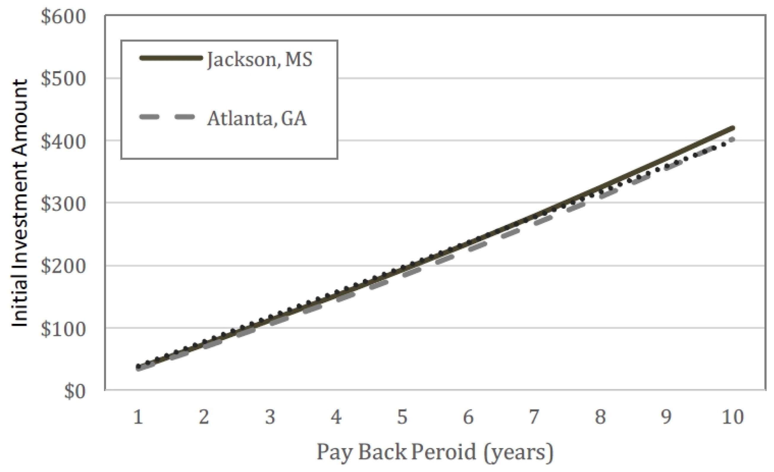
where $T_{amb}\left(t\right)$ is the ambient temperature, which is the hourly dry bulb temperature collected by the National Renewable Energy Laboratory for Jackson, MS [14]; and $T_{Building}$ is the internal temperature of the building.

The time constant of the building seen in Equation (2) is found by multiplying the envelope resistance, $R_{Building}$; by the thermal capacitance of the building, $C_{Building}$. The envelope resistance and thermal capacitance values were obtained from Lombard and Mathews [4].

$${\tau }_{Building}=R_{Building}\times C_{Building}$$

(2)

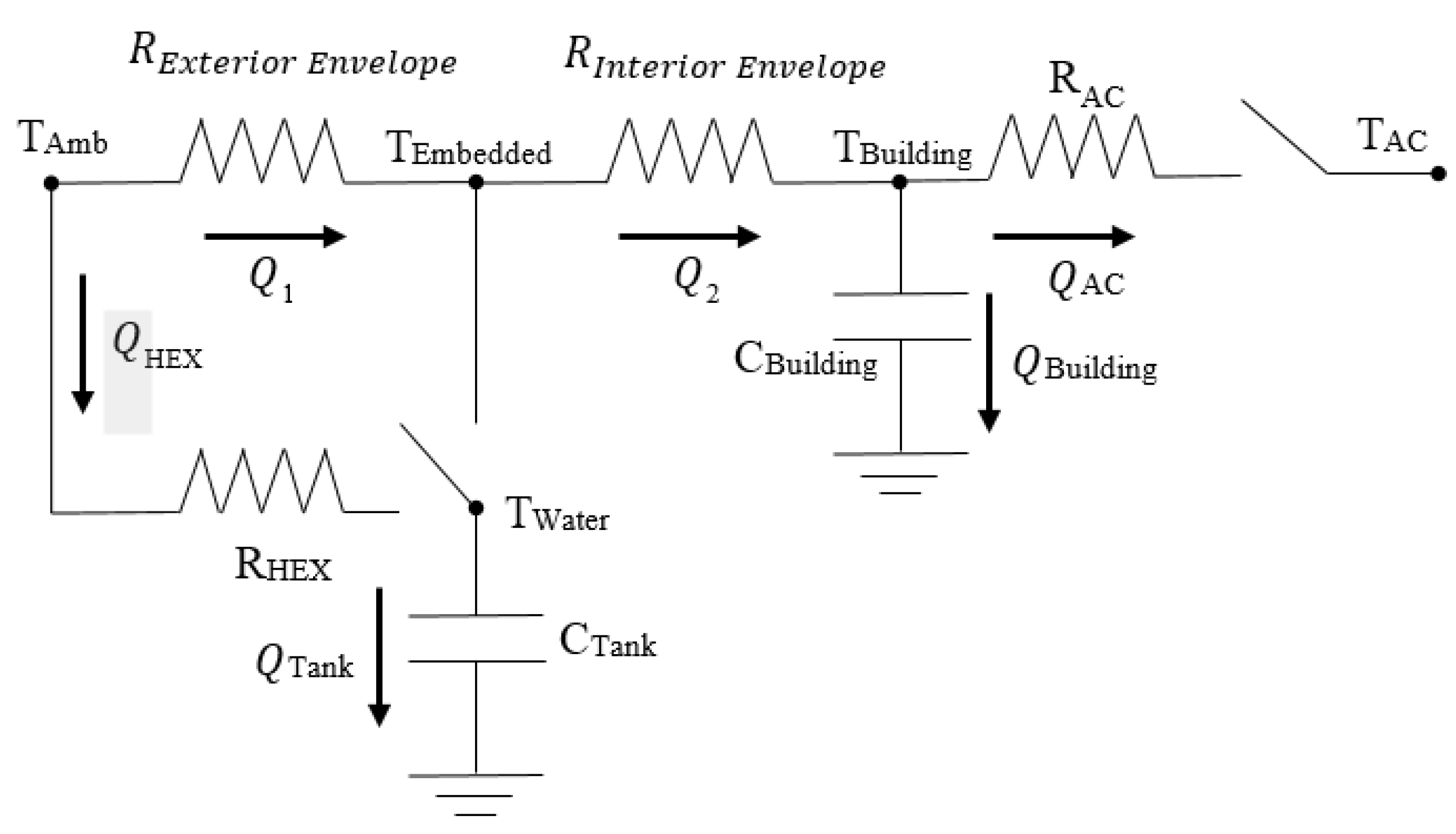
Preliminary simulations that were run in this study show that ITC is more beneficial when the piping for the ITC is placed close to the interior of the room. Following this idea, the thermal resistance of the building envelope is divided in two, resulting in an interior envelope and exterior envelope with piping for the ITC between these two regions. The exterior envelope, Equation (3), was selected to account for 90% of the thermal resistance, and the interior envelope, Equation (4), accounted for 10%, indicating that the water piping is closer to the interior side of the building.

$$R_1=R_{Exterior Envelope}=\frac{9}{10}\times R_{Building}$$

(3)

$$R_2=R_{Interior Envelope}=\frac{1}{10}\times R_{Building}$$

(4)

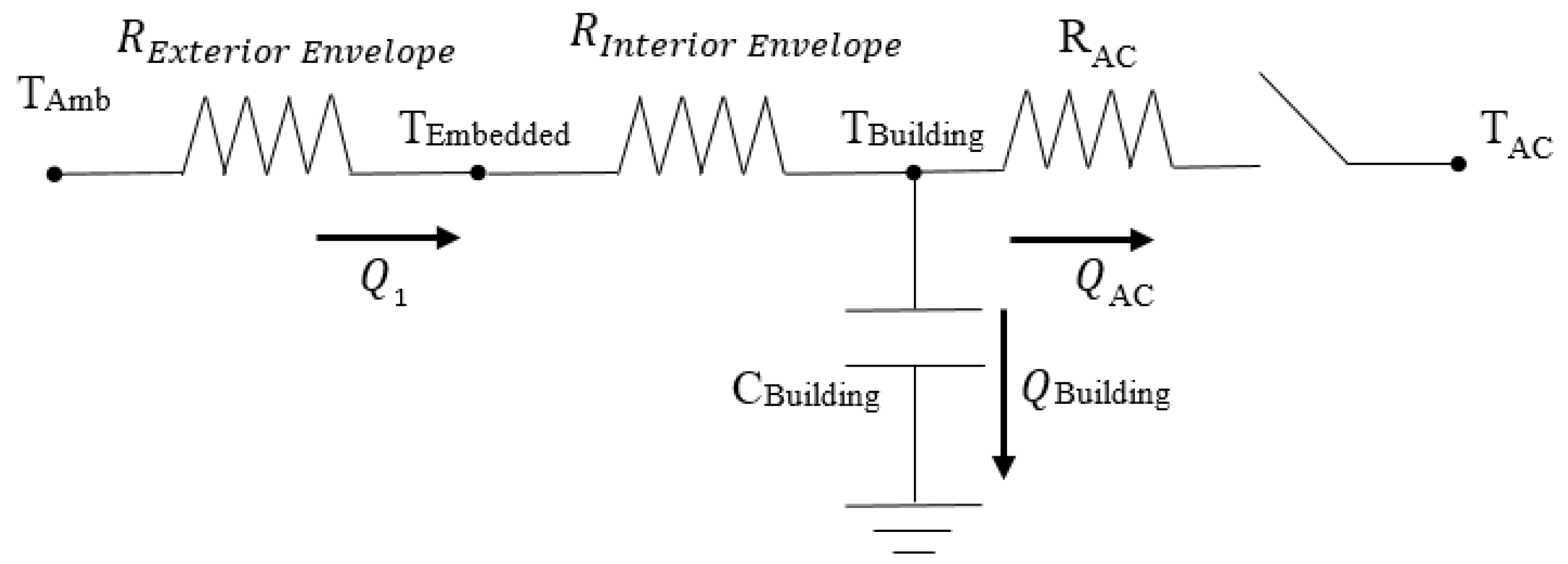
Although the reference model does not take advantage of the ITC, for comparison purposes, resistances for the exterior and interior envelopes are used in the reference model. The thermal circuit for the reference model is shown in Figure 1. $R_1$ and $R_2$ account for exterior and interior lumped thermal resistances, respectively. The AC system is modeled as room air circulating through constant-temperature cooling or heating coils. The resistance R_AC accounts for the net thermal resistance between the coil temperature and the temperature of the room air circulating through the coils. R_AC was selected by sizing an AC unit for an 11 m² building. A 2.64 kW (9000 Btu/h) unit was selected for this building [15]. Multiple air conditioner sizes were considered when calculating the AC resistance value, however larger units did not provide any considerable benefits. A 4.4 kW unit only affected the required energy of the AC subsystem by 3% and an 800 W unit increased the required energy by only 4%. R_AC resistance variations are explored in the sensitivity analysis discussed later in Section 3.1. The building properties used in the simulations are presented in Table 1. Details for the AC/heating subsystem are given in Section 3, and operating conditions and temperatures for the AC/heating subsystem can be found in Table 2 and Table 3.

Figure 1. Reference building circuit.

Figure 1. Reference building circuit.

Table 1. Building properties for a single room with brick cavity brick walls.

Building Properties	Values
Outer envelope resistance (R1)	2.6 × 10−2 K/W
Inner envelope resistance (R2)	2.9 × 10−3 K/W
HEX resistance (RHEX)	5.4 × 10−4 K/W
AC resistance (RAC)	2.7 × 10−3 K/W
Building capacitance (CBuilding)	4 × 106 J/K
Water tank capacitance (CTank)	2.4 × 107 J/K
Building time constant	32 h

Table 1. Building properties for a single room with brick cavity brick walls.

Building Properties	Values
Outer envelope resistance (R1)	2.6 × 10−2 K/W
Inner envelope resistance (R2)	2.9 × 10−3 K/W
HEX resistance (RHEX)	5.4 × 10−4 K/W
AC resistance (RAC)	2.7 × 10−3 K/W
Building capacitance (CBuilding)	4 × 106 J/K
Water tank capacitance (CTank)	2.4 × 107 J/K
Building time constant	32 h

Table 2. Constant operating temperature for the temperature node T_AC.

Operating Temperature	(°C)
Cooling	13
Heating	82

Table 2. Constant operating temperature for the temperature node T_AC.

Operating Temperature	(°C)
Cooling	13
Heating	82

Table 3. Upper and lower dead-band operation temperatures for T_Building.

	Cooling (May–September)	Heating (October–April)
8 am–8 pm on temperature	23 °C	22 °C
8 am–8 pm off temperature	21 °C	24 °C
8 pm–8 am on temperature	22 °C	22 °C
8 pm–8 am off temperature	20 °C	21 °C

Table 3. Upper and lower dead-band operation temperatures for T_Building.

	Cooling (May–September)	Heating (October–April)
8 am–8 pm on temperature	23 °C	22 °C
8 am–8 pm off temperature	21 °C	24 °C
8 pm–8 am on temperature	22 °C	22 °C
8 pm–8 am off temperature	20 °C	21 °C

The transient model consists of a state variable equation for a first-order lumped parameter system. The state variable, $T_{Building}$, represents the temperature of the lumped thermal capacitance of the building. A variable S is used as a flag to determine the operation of the AC/heating system. When S is equal to 1, the AC/heating subsystem is active, and when S is equal to 0, the AC/heating subsystem is inactive. Equation (5) shows the state variable equation for the internal temperature of the building, $T_{Building}$.

$$\frac{d{T}_{Building}}{dt}=\frac{1}{C_{Building}}\times Q_{Building}$$

(5)

where $Q_{Building}$ is the heat transfer through the building.

Depending on the season, i.e., warm season vs. cool season, the equation for $Q_{Building}$ varies; Equation (6) is used in the warm season requiring cooling, while Equation (7) is used in the cool season requiring heating. In both equations $T_{cooling}$ and $T_{heating}$ are constant set point temperatures and the rest of the temperatures are time-varying.

$$Q_{Building}=\{\begin{array}{cc}\frac{T_{amb}-T_{Building}}{R_1+R_2}-\frac{T_{Building}-T_{cooling}}{R_{AC}}& if S=1\\ \frac{T_{amb}-T_{Building}}{R_1+R_2}& otherwise\end{array}$$

(6)

$$Q_{Building}=\{\begin{array}{cc}\frac{T_{amb}-T_{Building}}{R_1+R_2}-\frac{T_{Building}-T_{heating}}{R_{AC}}& if S=1\\ \frac{T_{amb}-T_{Building}}{R_1+R_2}& otherwise\end{array}$$

(7)

The flag S was used in simulating the more realistic scenario of dead-bands in the AC and heating systems. The AC system begins to operate once the building temperature reaches the upper dead-band limit, $T_{Coolon}$. Once the temperature decreases below the upper dead-band limit, the AC system continues to operate while inside the dead-band region. Once the temperature reaches the lower limit, $T_{Cooloff}$, the AC will shut off and allow the ambient temperature to increase the building temperature until the upper limit is reached again. 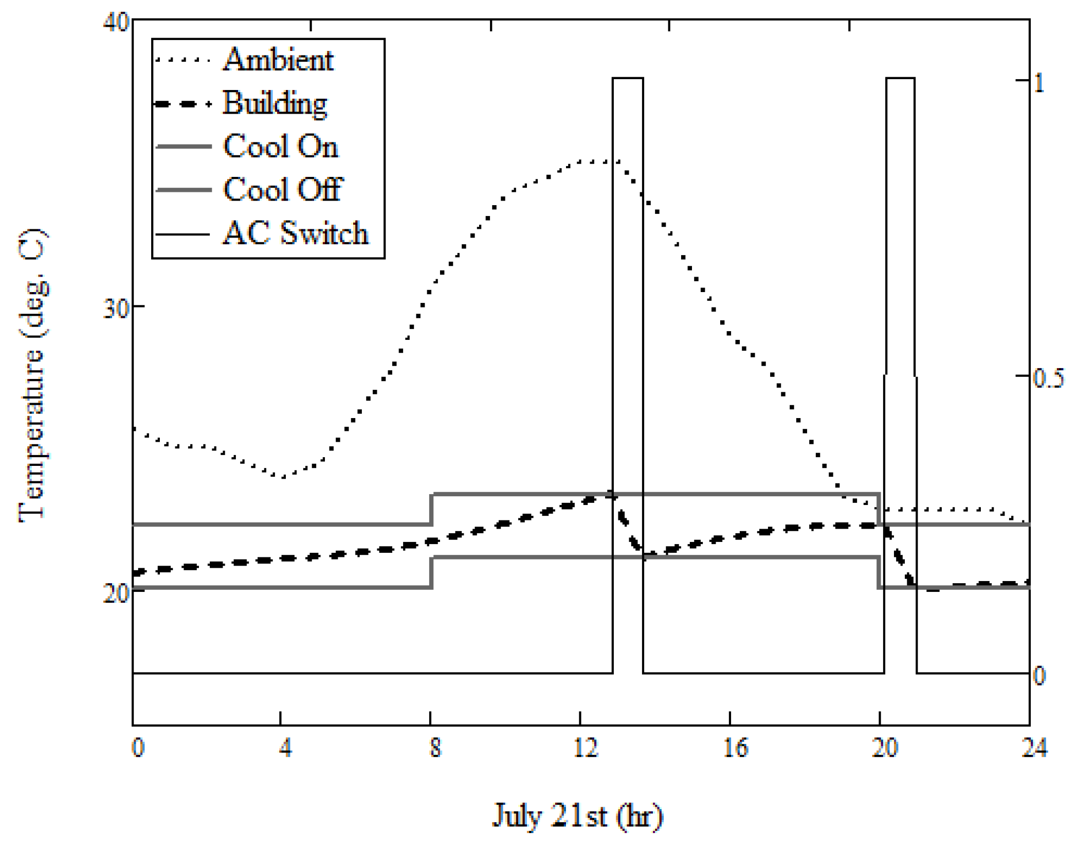Conversely, when using heating during the cool season, the simulation will allow ambient temperatures to lower the temperature of the building until the lower dead-band temperature limit, $T_{Heaton}$, is reached, then the heating will turn on and increase the building temperature until it reaches the high dead-band temperature limit, $T_{Heatoff}$, and the heating turns off. An example of the AC operating with a dead-band for 21 July can be seen in Figure 2. In addition, the ambient, building, cool on, and cool off temperatures are also illustrated in this figure. The dead-band shifting at 8 am and 8 pm is to simulate a typical residential building where the occupant desires to save energy and allows the building to reach a higher temperature while it is unoccupied. Some differential equation solvers do not allow to track time-varying variables other than state variables. For this reason, in order to track the value of S, a state variable equation for S was developed assuming that the simulation time step is constant. The state variable equation for S during the warm season and the cool season can be seen below in Equations (8) and (9), respectively. The equations were created such that the value of S can change between 0 and 1 within a single time step of Δt.

Figure 2. Air Conditioning Example from July 21st.

Figure 2. Air Conditioning Example from July 21st.

$$\frac{dS}{dt}=\{\begin{array}{cc}\frac{-S+1}{\Delta t}& if T_{Building}\ge T_{Coolon}\\ \frac{-S}{\Delta t}& if T_{Building}\le T_{Cooloff}\\ 0& otherwise\end{array}$$

(8)

$$\frac{dS}{dt}=\{\begin{array}{cc}\frac{-S+1}{\Delta t}& if T_{Building}\le T_{Heaton}\\ \frac{-S}{\Delta t}& if T_{Building} \ge T_{Heatoff}\\ 0& otherwise\end{array}$$

(9)

For all the simulations presented in this paper, Δt is 0.2 min, i.e., there are 5 data points of the building temperature and the state of the AC taken every minute.

A third state variable equation was added to integrate the heat rate from the AC, $Q_{AC}$, such as to determine the total energy extracted, $E_{AC}$, by the AC subsystem. Similarly, during the cool season, the total energy added, $E_{Heat}$, by the heating subsystem is obtained by integrating the heat rate from the heater, $Q_{Heat}$. The state variable equations for each case are shown below in Equations (10) and (11).

$$\frac{d}{dt}{E}_{AC}=Q_{AC}=\{\begin{array}{cc}\frac{T_{Building}-T_{cooling}}{R_{AC}}& if S=1\\ 0& otherwise\end{array}$$

(10)

$$\frac{d}{dt}{E}_{Heat}=Q_{Heat}=\{\begin{array}{cc}\frac{T_{heating}-T_{Building}}{R_{AC}}& if S=1\\ 0& otherwise\end{array}$$

(11)

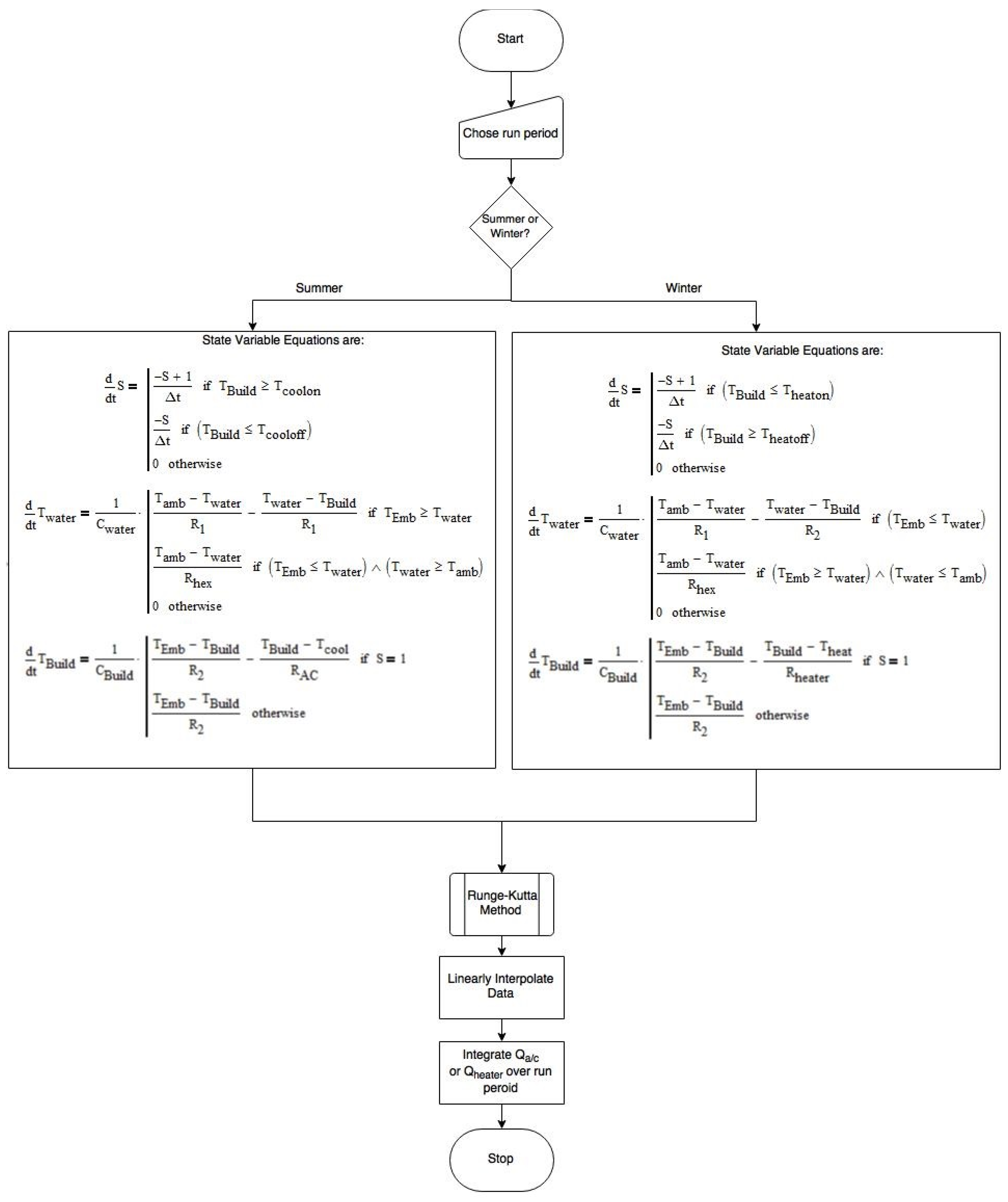
In summary, the system of first order ordinary differential equations, i.e., state variable equations, solved during the cooling season is composed of Equations (6), (8), and (10). Conversely, the state variable equations solved during the heating season are composed of Equations (7), (9), and (11). To avoid errors in selecting the initial building temperature, numerical data was collected only after the first 24 h of simulation, once the effects of the initial conditions subsided.

2.2. Increased Thermal Capacitance with Thermal Storage Management Model

A second circuit was developed to study how the ITC/TSM system can reduce the operating time for the AC system and the heating system. The ITC/TSM as described in Figure 3, has the same lumped thermal capacitance of the building presented in Section 2.1, but, in addition, copper pipes carrying water are embedded between the inner and outer building envelopes. A heat exchanger exposed to ambient temperatures was also added to improve the temperature of the water in the tank whenever favorable. For instance, during warm seasons, the water will circulate through the external heat exchanger if the ambient temperature is lower than the temperature in the water tank, and during the cold seasons the water will circulate through the heat exchanger when the ambient temperature is higher than the water tank temperature.

Figure 3. ITC/TSM building circuit.

Figure 3. ITC/TSM building circuit.

This thermal storage system saves energy for the entire system by taking advantage of the climate. Using the properties of copper piping found in [3] and the building envelope properties found in [4], it was found that the envelope resistance is 200 times greater than the resistance of the copper pipe; therefore, the copper piping’s contribution to the net resistance will be omitted in this first order analysis. As with the reference model, the thermal building envelope resistance is also split into two sections, R₁ and R₂. The pipes allow water to circulate through the building and back to a storage tank. This tank has a volume of approximately 5.7 m³ (1500 gallons). The total water in the pipes and in the storage tank increases the thermal capacitance of the building presented in Section 2.1 by a factor of six. The water tank capacitance was calculated using the specific heat, density and volume of the water in the tank. The sensitivity of the results to the tank size are presented later in Section 3.1.

The time constant for the building was significantly increased by the addition of the water tank. The time constant was also found from the simulation results by disconnecting the AC system and setting the ambient temperature to a constant value that will decay the building temperature to zero i.e., $T_{Amb}=0$. Equation (12) below was used to solve for the time constant obtained from the lumped parameter models.

$$T_{Building}\left(t\right)=T_{Building}\left(0\right)\times e^{-\frac{t}{\tau }}$$

(12)

where $T_{Building}$ is the temperature of the building at a given time; and $T_{Building}\left(0\right)$ is the initial temperature of the building. Equation (12) was rearranged to solve for the time constant as follows:

$$\tau =\frac{-t}{\text{ln}\left(\frac{T_{Building}\left(t\right)}{T_{Building}\left(0\right)}\right)}$$

(13)

2.2.1. Verification of the Time Constants Using TRNSYS

Transient simulations using the software TRNSYS 17 [16] were conducted to verify the magnitude of the time constants used in the lumped parameter system presented in this paper. A detailed model was constructed using the software TRNSYS 17. The reference building was simulated using predefined standard ASHRAE wall, roof and flooring materials provided by the TRNSYS library. The walls were double brick as defined in Lombard and Mathews and have a standard thickness of 92 mm [17]. A constant weather input temperature of 10 °C was used when determining the time constant. The time constant was obtained from the response from the TRNSYS 17 assuming that after some time, transients with smaller time constant will decay and the dynamics of the response will follow the dominant time constant. Equation (14) was used to model the response of the dominant time constant of the TRNSYS 17 model, assuming the response to faster time constants has already decayed.

$$T_{Building}\left(t\right)=A\times e^{\frac{-t}{\tau }}+C$$

(14)

where C is the constant weather temperature; and A is a constant of integration. For purely first order systems $A=T_{Building}\left(0\right)$ is the initial temperature of the building, but for a higher order model consisting of several time constants, the value of A associated with the dominant time constant will not necessarily be equal to $T_{Building}\left(0\right)$.

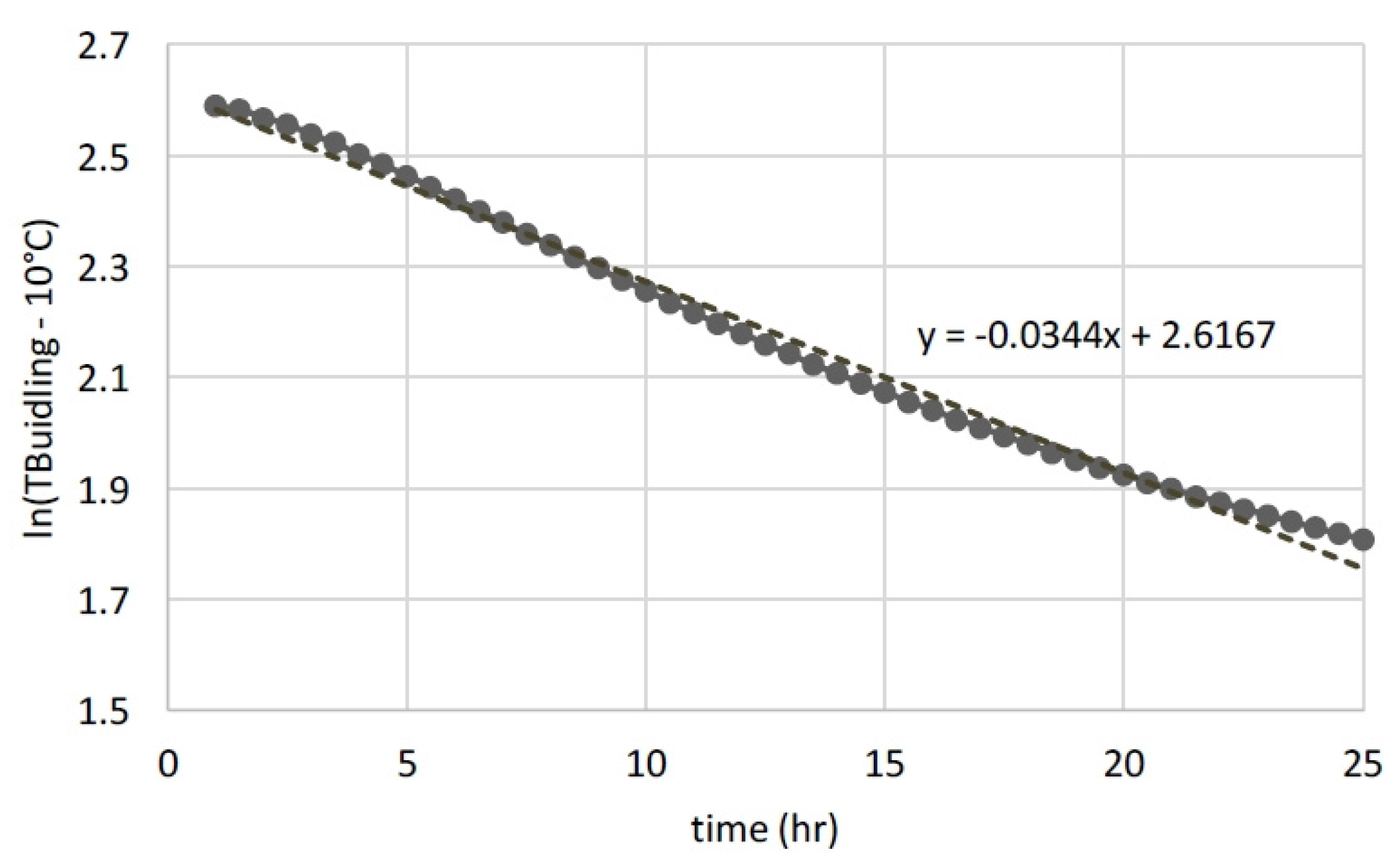
In order to extract the time constant information from the data obtained from TRNSYS 17 model, the above equation was rearranged as shown in Equation (15) where it is shown that the slope of the curve obtained by plotting the data in a semilog plot, i.e., as $\text{ln}\left(y-C\right)$ vs. t, is the inverse of the time constant. Figure 4 shows this plot and the trendline used to calculate the time constant. It was found that the time constant was 29 h, which is consistent with the initial calculated time constant for the reference building of 32 h and provides verification for the seemingly large value.

$$\text{ln}\left(T_{Building}-C\right)=\text{ln}\left(A\right)-\frac{1}{\tau }\times t$$

(15)

Figure 4. Trendline used to calculate the time constant for the TRNSYS simulation.

Figure 4. Trendline used to calculate the time constant for the TRNSYS simulation.

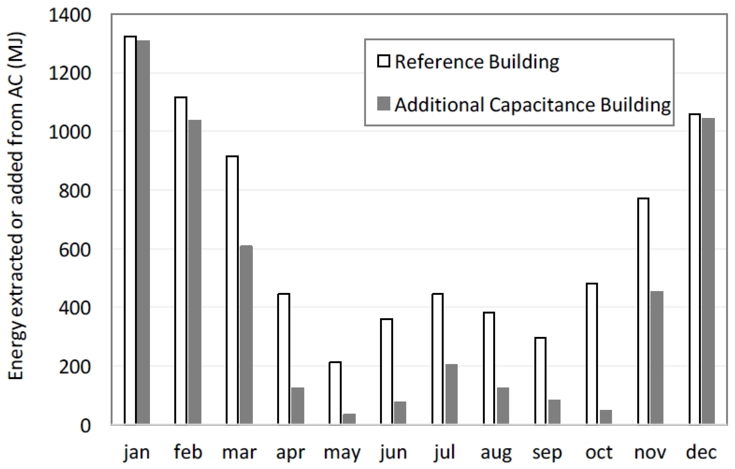
The second TRNSYS simulation used the same building that was constructed for the time constant verification, but TMY2 weather data was used during the simulation rather than the constant temperature input. Only the dry bulb temperature of Jackson, MS was used, and it was applied to the ambient temperature. It should be noted that all effects from radiative heat transfer have been neglected in both the TRNSYS simulation and the circuit analysis. The heat extracted by the building was collected for the months of February and July for both methods of solving the system. For the month of February, the TRNSYS simulation required 1246 MJ of heating and the circuit analysis required 1171 MJ, a 6% difference between the two simulations. During the month of July the TRNSYS simulation required 480 MJ of cooling and the circuit analysis required 446 MJ, a 7.1% difference between the two simulations.

2.2.2. Operation of the ITC/TSM System

The ITC/TSM system is based on three modes of operation. In Mode 1 water is circulated through the water tank and the building. In Mode 2, water is only circulated between the water tank and the heat exchanger. Mode 3 corresponds to the inactive state, where water is not circulated through the building or the heat exchanger. Mode 3 is used exclusively for storage. In all modes, the original capacitance of the building is used when calculating the room temperature. In Figure 3, the heat exchanger is modeled as a single resistance in series with the ambient temperature. The value of this resistance, seen in Table 1, was calculated by sizing a water-to-air heat exchanger [18] and by using the ambient and water temperatures.

$T_{Embedded}$ is the temperature at the location where the water pipes are embedded within the envelope thermal resistance. The requirements for circulating water through the building depend on $T_{Embedded}$, the temperature of the water in the water tank, and the season. During warm months, May through September, the water circulates if $T_{Embedded}$ is greater than the temperature in the water tank. When water circulation from the tank capacitance is disconnected from the building envelope, the resulting $T_{Embedded}$ in Equation (16) is found using a “voltage divider” equation across the inner and outer envelope resistances, $R_1$ and $R_2$, between the ambient temperature and the temperature of the building. Otherwise, the $T_{Embedded}$ is assumed to be at the same temperature as the water tank temperature, $T_{Water}$. All temperatures in Equation (16) are time-varying.

$$T_{Embedded}=\{\begin{array}{l}{T}_{Water} if \left(T_{amb}-\frac{T_{amb}-T_{Building}}{R_1+R_2}\times R_1\right)\ge T_{Water}\hfill \\ \left(T_{amb}-\frac{T_{amb}-T_{Building}}{R_1+R_2}\times R_1\right) otherwise\hfill \end{array}$$

(16)

During the cool months, October through April, the operation of the ITC/TSM is opposite of that in the warm months, resulting in Equation (17).

$$T_{Embedded}=\{\begin{array}{l}{T}_{Water} if \left(T_{amb}-\frac{T_{amb}-T_{Building}}{R_1+R_2}\times R_1\right)\le T_{Water}\hfill \\ \left(T_{amb}-\frac{T_{amb}-T_{Building}}{R_1+R_2}\times R_1\right) otherwise\hfill \end{array}$$

(17)

The temperature of the water in the water tank, $T_{Water}$, is an additional state variable described in Equation (18) where $Q_{Water}$ represents the heat transferred into the water.

$$\frac{d{T}_{Water}}{dt}=\frac{1}{C_{Water}}\times Q_{Water}$$

(18)

There are two equations associated with $Q_{Water}$, one for the warm season and one for the cool, shown in Equations (19) and (20), respectively.

$$Q_{Water}=\{ \begin{array}{l}\frac{T_{Amb}-T_{Water}}{R_1}-\frac{T_{Water}-T_{Building}}{R_2} if T_{Embedded}\ge T_{Water}\hfill \\ \frac{T_{Amb}-T_{Water}}{R_{HEX}} if \left(T_{Embedded}\le T_{Water}\right) and \left(T_{Water}\ge T_{Amb}\right)\hfill \\ 0 otherwise\hfill \end{array}$$

(19)

$$Q_{Water}=\{\begin{array}{l}\frac{T_{Amb}-T_{Water}}{R_1}-\frac{T_{Water}-T_{Building}}{R_2} if T_{Embedded}\le T_{Water}\hfill \\ \frac{T_{Amb}-T_{Water}}{R_{HEX}} if \left(T_{Embedded}\ge T_{Water}\right) and \left(T_{Water}\le T_{Amb}\right)\hfill \\ 0 otherwise\hfill \end{array}$$

(20)

Equations (21) and (22) describe the heat rate to the building, $Q_{Building}$, during warm and cool seasons, respectively.

$$Q_{Building}=\{\begin{array}{l}\frac{T_{Embedded}-T_{Building}}{R_2}-\frac{T_{Building}-T_{cooling}}{R_{AC}} if S=1\hfill \\ \frac{T_{Embedded}-T_{Building}}{R_2} otherwise\hfill \end{array}$$

(21)

$$Q_{Building}=\{\begin{array}{l}\frac{T_{Embedded}-T_{Building}}{R_2}-\frac{T_{Building}-T_{heating}}{R_{AC}} if S=1\hfill \\ \frac{T_{Embedded}-T_{Building}}{R_2} otherwise\hfill \end{array}$$

(22)

To avoid errors in selecting the initial building temperature, numerical data was collected only after the first 8 days of simulation, once the effects of the initial conditions have subsided. This is greater than the reference case because of the increased time constant. Note that this is only one time constant, not the typical 5 τ that is required for a simulation to fully reach steady-state. Reducing the computational time only affected the collected data by 0.17%. This was found by comparing the extracted energy on 21 July with 8 days of simulation and 50 days of simulation prior to collecting data.

A summary of the state variables equations and the process used when solving these equations can be seen in the flowchart shown in Figure 5.

2.3. Cooling and Heating Subsystem

The cooling system operates only for the months of May through September, and the heating system operates from October through April. The cooling and heating system each operate at a constant temperature and were modeled as a single temperature node (T_AC) and resistance (R_AC) since they would never operate simultaneously. This constant temperature node is intended to represent a working fluid, such as water or a refrigerant, coming in contact with heating or cooling coils. These constant temperatures are listed in Table 2. The AC operates on a cycle. During the evening hours, from 8 pm to 8 am, the house is kept at a cooler temperature than during the day hours, i.e., from 8 am to 8 pm. Occupational Safety and Health Administration (OSHA) requires that a workplace temperature must be kept in the range of 20 °C to 24 °C [19]. Thus the average daytime summer temperature was chosen to be 22 °C with an on/off cycle of 1 °C, i.e., the cooling system begins to operate when the building reaches 23 °C and stops operating when the building temperature drops to 21 °C. The heating system operates in a similar fashion, but the off temperatures are set slightly higher to allow the building to reach a higher temperature during the winter. Table 3 lists the upper and lower limit building temperatures.

Figure 5. Flowchart for state variable equations for the ITC/TSM system.

Figure 5. Flowchart for state variable equations for the ITC/TSM system.

3. Results and Discussion

Simulations were performed to provide a month-by-month comparison of the heat rate associated with the AC of each circuit. The total energy transferred each month was calculated by numerically integrating the heat transfer rate, Q_AC, over the month. Figure 6 displays absolute values and does not distinguish between whether the energy is extracted or added to the building. The energy extracted by the AC system is a result of the cooling system operating, May through September, and the energy added to the building is the result of the heating system operating between the months of October through April. For the months of March through November, there are significant benefits from using the ITC/TSM system, but the simulation shows that there are only slight benefits from using the system from December through February. One reason the additional capacitance system is not beneficial during the winter months is because the ambient temperature does not reach a high enough temperature to assist with warming up the water. If the water temperature at the water tank, $T_{Water}$, is lower than the embedded temperature, $T_{Embedded}$, the water will not circulate through the building and the building operates using the heating system in the same manner as the reference case. Though the system is not very beneficial for three months of the year, the benefits that occur during the 9 remaining months compensate for these winter months. May through September, the average reduction of the AC energy requirement is about 70% and May alone has a reduction of nearly 85%.

Figure 6. Energy required for reference building and ITC/TSM building.

Figure 6. Energy required for reference building and ITC/TSM building.

All monthly energy requirements can be seen in Figure 6. Though May has a high percentage of energy reduction, the month of October has the greatest reduction of energy required. The month of May does not heavily rely on the use of the AC subsystem and the ITC/TSM system almost eliminates the need for the AC subsystem completely. However, the month of October does rely on the use of the heating system, and the ITC/TSM system is able to provide the greatest reduction in required extracted/added energy. A month-by-month comparison for the difference in energy for the reference system and the ITC/TSM can also be seen in Figure 7.

Figure 7. The difference in required energy and the percent energy reduction.

Figure 7. The difference in required energy and the percent energy reduction.

The spike in the heat transfer rate through the heating system during the winter months can be explained by the difference between AC/heater temperature and the building temperature for the summer versus the winter. During the summer this temperature difference is roughly 9 °C and in the winter this temperature difference is 60 °C. Since the AC/heater resistance remains constant, the heat transfer rates depend on the temperature difference between the building and the AC/heater operating temperature. Therefore, it takes more energy to heat the house during the winter than it does to cool the house during the summer.

3.1. Sensitivity Analysis

A sensitivity analysis was conducted for the following variables: the heat exchanger resistance, the AC/heating resistance, the building capacitance and the tank capacitance. The sensitivity analysis used 21 January for the simulation day and was conducted only for the circuit with the ITC/TSM system. Table 4 shows a summary of the variables which were altered and the resulting effect on the simulation. Each chosen variable was increased and decreased by 3% to show that it did not have a large impact on the calculation of the energy added by the heater. Increasing and decreasing each variable by 3% had less than a 2.3% effect on the energy added by the heater. The largest variance was from the increased building capacitance. This was expected since this effectively increases the building’s mass and thus increases the required energy to maintain thermal comfort. All other variables, including the tank size, have less than a 0.6% effect on the energy added to the system.

Table 4. Sensitivity analysis results.

Variable	Modified Amount	Percent Change from Original Energy Added by Heater
Heat exchanger resistance	Increased 3%	0.07%
	Decreased 3%	−0.6%
Heater resistance	Increased 3%	0%
	Decreased 3%	−0.53%
Building capacitance	Increased 3%	2.1%
	Decreased 3%	−2.3%
Water tank capacitance	Increased 3%	0.07%
	Decreased 3%	−0.6%

Table 4. Sensitivity analysis results.

Variable	Modified Amount	Percent Change from Original Energy Added by Heater
Heat exchanger resistance	Increased 3%	0.07%
	Decreased 3%	−0.6%
Heater resistance	Increased 3%	0%
	Decreased 3%	−0.53%
Building capacitance	Increased 3%	2.1%
	Decreased 3%	−2.3%
Water tank capacitance	Increased 3%	0.07%
	Decreased 3%	−0.6%

3.2. Economic Analysis

This section addresses the potential economic benefits of the proposed system. Three different cities were considered during the economic analysis: Jackson, MS; Jacksonville, Florida; and Atlanta, Georgia. This was done to show that the proposed system could be beneficial for climates similar to Jackson MS. An initial investment amount to install the proposed system was calculated by selecting the number of years desired for the payback period. To calculate the electricity consumption, the following equation was used [20]:

$$Electricit{y}_{in}\left[W\right]=\frac{Coolin{g}_{power}\left[\frac{BTU}{hr}\right]}{EER or HSPF}$$

(23)

where EER is the energy efficiency ratio and HSPF is the heating seasonal performance factor. As can be seen from Equation (23), the electricity consumption will strongly depend on the system selected, which will have different EER and HSPF values. For illustration purposes, a system with a typical average EER of 13 and an average HSPF of 10 was selected to estimate the potential savings and the initial investment amount that would be available to install the proposed system. During the cool season the HSPF value was used during calculations and during the warm season the EER value was used to calculate the require electricity.

Both the reference case and the ICT/TSM systems were simulated for a full year and the difference in electricity consumption between the two was multiplied by the electricity cost for each state. Electricity costs were taken from the U.S. Energy Information Administration [21]. To account for the inflation of the electricity cost, the increase in electricity cost was considered for the five previous years. The average of the percent increase for each year was the value used during the calculations, and these values and the electricity cost for each city are presented in Table 5. The ITC/TSM system was able to reduce the operating costs of the Jackson, Atlanta, and Jacksonville buildings by 31%, 23%, and 44%, respectively. Figure 8 shows the initial investment amount available to install the proposed system for payback periods up to 10 years. It can be seen that Jackson does produce the largest initial investment, though Atlanta and Jacksonville provide similar results. Though these initial investments might seem inadequate, they are due to the building being very small, and are limited by the fact that the building does not require much electricity to operate.

Table 5. Average retail price of electricity to residential sector, July 2014–2010 [21].

State	2014 (Cents/kWh)	2013 (Cents/kWh)	2012 (Cents/kWh)	2011 (Cents/kWh)		2010 (Cents/kWh)	Average % increase
Mississippi	11.63	10.88	10.07	10.41	10.29		3%
Georgia	12.55	12.31	11.96	12.07	10.95		4%
Florida	11.96	11.39	11.56	11.82	11.72		1%

Table 5. Average retail price of electricity to residential sector, July 2014–2010 [21].

State	2014 (Cents/kWh)	2013 (Cents/kWh)	2012 (Cents/kWh)	2011 (Cents/kWh)		2010 (Cents/kWh)	Average % increase
Mississippi	11.63	10.88	10.07	10.41	10.29		3%
Georgia	12.55	12.31	11.96	12.07	10.95		4%
Florida	11.96	11.39	11.56	11.82	11.72		1%

Figure 8. Initial investment amount (USD) per payback period.

Figure 8. Initial investment amount (USD) per payback period.

This analysis can be extrapolated to a bigger building in which the proposed system would potentially provide more savings and the initial investment to install the proposed system would be higher. In addition, the same estimation can be done for different systems that would have different values of EER and HSPF.

4. Conclusions

The purpose of this study was to determine if the proposed ITC/TSM system could potentially reduce the energy required for thermal comfort in a building. This was achieved by comparing two circuits, a reference circuit and a circuit implementing the ITC/TSM system, both simulated for a year to determine the energy required by the AC/heating subsystem. The first-order simulations determined that there were significant reductions in the energy consumption of the AC subsystem when the ITC/TSM system was used in a simple one-room micro building with climate conditions corresponding to Jackson, Mississippi. However, since the simulations correspond to a first-order model approximation, the benefits would likely not be as large as the 70% reduction seen during summer operation. The largest monthly reductions for the evaluated ITC/TSM system occur in the months of March through November. It is expected that the ITC/TSM system would be able to deliver a similar performance for locations with climate conditions similar to these months, as reference temperatures during these seasons reach as high as 37 °C, and as low as −7 °C in the beginning of March and at the end of October. The ITC/TSM is frequently active in Mode 1 or Mode 2 and is occasionally operating in Mode 3, the inactive state, which is equivalent to the reference case. The greatest benefits are gained from the ITC/TSM system when the building does not operate in Mode 3. The ITC/TSM system is often active from March to October, which suggests that a significant portion of these months consistently take advantage of ITC/TSM system. Future work will include incorporating a phase change material into the tank to further control the water temperature, integrating radiative heat transfer from the ambient conditions to provide a more accurate simulation, modifying the model to include various types of buildings and providing an experimental verification of the analytical simulations using a micro building.

References

1. Karlssoon, J. Possibilities of Using Thermal Mass in Buildings to Save Energy, Cut Power Consumption Peaks and Increase the Thermal Comfort; Licentiate; Lund Institute of Technology: Lund, Sweden, 2012. [Google Scholar]
2. Rearson, C.; McGee, C.; Milne, G. Thermal mass. In Your Home: Australia’s Guide to Environmentally Sustainable Homes; Department of Industry: Sydney, Australia, 2013; pp. 178–187. [Google Scholar]
3. Carpenter, J.; Mago, P.; Luck, R.; Cho, H. Passive energy management through increased thermal capacitance. Energy Build. 2014, 75, 465–471. [Google Scholar] [CrossRef]
4. Lombard, C.; Mathews, E.H. Efficient, steady state solution of a time variable RC network, for building thermal analysis. Build. Environ. 1992, 27, 279–287. [Google Scholar] [CrossRef]
5. Madhumathi, A.; Sundarraja, M.C. Energy efficiency in buildings in hot humid climatic regions using phase change materials as thermal mass in building envelope. Energy Environ. 2014, 25, 1405–1421. [Google Scholar] [CrossRef]
6. Zhu, N.; Wang, S.; Xu, X.; Ma, Z. A simplified dynamic model of building Structures integrated with shaped-stabilized phase change materials. Int. J. Therm. Sci. 2010, 49, 1722–1731. [Google Scholar] [CrossRef]
7. Tan, S.; Yu, S.; Xu, G.; Zhang, Y. Preparation and properties studies of paraffin/high density polyethylene composites and phase-change coatings. Process Org. Coat. 2013, 76, 1761–1764. [Google Scholar] [CrossRef]
8. Shi, Y.; Wu, Y.; Zhu, L.; Shentu, B.; Weng, Z. Preparation and properties of phase-change heat-storage UV curable polyurethane acrylate coating. J. Appl. Polym. Sci. 2014, 132, 41266. [Google Scholar] [CrossRef]
9. Tarnai, T. Geodesic Domes: Natural and man-made. Int. J. Space Struct. 2011, 26, 215–227. [Google Scholar] [CrossRef]
10. Standridge, T. Building a desert dwelling. Countrys. Small Stock J. 2013, 97, 29–37. [Google Scholar]
11. California Energy Commission. New Residential Zero Net Energy Action Plan 2014–2020, CA Energy Efficiency Strategic Plan; State of California: San Francisco, CA, USA, 2013.
12. Cater, F. Living Small in the City: With More Singles, Micro-Housing Gets Big, 26 February 2015. Available online: http://www.npr.org/2015/02/26/389263274/living-small-in-the-city-with-more-singles-micro-housing-gets-big (accessed on 6 June 2015).
13. Netfirms, NOMAD Micro Homes. NOMAD Micro Homes Inc. Available online: http://www.nomadmicrohomes.com (accessed on 6 June 2015).
14. U.S. Department of Energy. Brief Summary of the TMY2s, National Renewable Energy Laboratory, 2014. Available online: http://www.nrel.gov/rredc (accessed on 20 January 2015).
15. AC4Life. Air Conditioning Sizing Calculator, AC Direct, 2014. Available online: http://www.acdirect.com (accessed on 27 January 2015).
16. Solar Energy Laboratory, University of Wisconsin-Madison. TRNSYS Transient System Simulation Tool, 17th ed.; University of Wisconsin-Madison: Madison, WI, USA, 2009. [Google Scholar]
17. The Belden Brick Company. Brick Dimensions Guide, Belden Brick Company, 2013. Available online: http://www.beldenbrick.com (accessed on 6 June 2015).
18. Hydraulic Heating Supplies. Heat Exchangers, Water to Air Heat Exchangers, 2015. Available online: http://www.northlanddistrib.com (accessed on 27 January 2015).
19. OSHA. OSHA Technical Manual Section III: Chapter 2, Indoor Air Quality Investigation, 1990. Available online: http://www.osha.gov (accessed on 14 January 2015).
20. The Engineering ToolBox. Heat Pumps Performance and Efficiency Ratings, 2015. Available online: http://www.engineeringtoolbox.com/ (accessed on 6 June 2015).
21. U.S. Department of Energy. Electric Power Monthly, U.S. Energy Information Administration. Available online: http://www.eia.gov/electricity/monthly (accessed on 6 June 2015).