Co-Movement Analysis of Italian and Greek Electricity Market Wholesale Prices by Using a Wavelet Approach

Abstract

We study the co-evolution of the dynamics or co-movement of two electricity markets, the Italian and Greek, by studying the dynamics of their wholesale day-ahead prices, simultaneously in the time-frequency domain. Co-movement is alternatively referred as market integration in financial economics and markets are internationally integrated if the reward for risk is identical regardless the market one trades in. The innovation of this work is the application of wavelet analysis and more specifically the wavelet coherence to estimate the dynamic interaction between these two prices. Our method is compared to other generic econometric tools used in Economics and Finance namely the dynamic correlation and coherence analysis, to study the co-movement of variables of the type related to these two fields. Our study reveals valuable information that we believe will be extremely useful to the authorities as well as other agents participating in these markets to better prepare the national markets towards the European target model, a framework in which the two markets will be coupled.

1. Introduction

The Greek and Italian wholesale electricity markets are about soon to be coupled within the framework of the European Electricity Target Model (TM), a major theme of the 3rd package (published on 14 August 2009, in the Official Journal of the EC, and its provisions came into force on 2 March 2011) [1] of European Energy legislation. The coupling of prices of different markets, in the framework of TM, requires first a deep understanding of the dynamics of prices in each market (analysis is of stylized facts or statistical characteristics of the time variation of price volatility etc.). Therefore, modeling and prediction of day-ahead, wholesale electricity prices is considered a sine qua non prerequisite for understanding their dynamic evolution [2,3]. An even more important issue, when considering the possible coupling of two electricity markets, is the analysis of their price co-movement. The findings from such an analysis, as the authors consider, will contribute constructively on the gap analysis between the Target Model and the current Greek market design, which is under development (the Italian-Greek border will be technically ready for market coupling at a later date. The go-live date of this market coupling will be decided as soon as its technical readiness to enter has been assessed within the Italian borders market coupling project).

The Greek and Italian electricity markets are two distinct complex systems, each one with a different structure, having interacting agents with different term objectives. Their dynamic evolutions correspond to processes that have time series formed by a mixture of different components operating at different frequencies. Typical time series and econometric analysis toolboxes examine frequency and time component separately. An innovative approach of simultaneous analysis in time and frequency domains is the wavelet analysis. This approach helps us to reveal hidden interactions that are difficult to detect using typical econometric tools. An advantage of the wavelet analysis is that this is a model-free method.

Wavelets have been used extensively in analyzing financial and commodity markets [4,5]. In commodity markets beginning with recent works, Voronin et al. [6] proposed an iterative forecasting methodology for prediction of normal prices as well as price spikes in the day-ahead Nordic electricity market. The methodology included a mixture of wavelet transform, ARIMA and nonlinear network models. Naccache [7] has studied the co-movement of oil prices and economic activity using wavelet. The wavelet approach, in combination with ARIMA and GARCH models, has been used in analyzing and forecasting historical day-ahead electricity prices on Spanish and PJM (Pensilvania, New Jersey, Maryland) (PJM is a regional transmission organization (RTO), that coordinates the movement of wholesale electricity in all parts of 13 states and in the district of Columbia, USA) electricity markets [8]. Connor and Rossiter [9] estimated price correlations by decomposing, via wavelet, time series of commodity prices. In the same year, Yousefi et al. [10] predicted future oil prices using this method. Early, in 1997, Davidson et al. [11], was the first to propose a semi-nonparametric regression, using wavelets, to study the dynamics of commodity price. Literature on the issue of the dynamics of energy commodity is divided in three groups: Analysis of specific commodity time series, analysis of the macroeconomic relationships of commodities and finally analysis of the dynamics of co-movement between two commodities.

A good example of the aforementioned second group of literature, regarding the macroeconomic dependence of commodities is the work of Goshray and Johnson [12]. They study trends in world energy prices by using extensive data and institutional backgrounds and found that there exist co-movements between energy commodities, but not between two different electricity markets. In the work of Grine and Diko [13] the authors use an affine jump-diffusion modeling framework to capture the strong link between electricity prices and oil, coal and natural gas prices, and have indicated how these different markets commove via their price coupling. An extremely interesting and useful case, both from an academic and practical perspective, is the co-movement or co-evolution of two neighboring (adjacent) interconnected or integrated electricity markets, but this case has been rarely studied. The work of Cianneta and Zarrage [14] refers to such a co-movement, in the form of transmission of volatility of prices between two adjacent markets. More specifically, by using Constant (CCC) and Dynamic Conditional Correlation (DCC) (for the approach see Section 3.3 below) bivariate models, with three different models (specifications) of the univariate variance processes (a GARCH(1,1) structure), they studied the coevolution of the electricity markets of Spain and Portugal (they were integrated in 2007 to create the Iberian electricity market, OMIE), as well as the coevolution of French and Spanish, interconnected markets. However, in their work, the co-movements are analyzed only in time, not in frequency, by detecting the time-varying dynamic correlation of prices, between the two markets.

To the best of our knowledge, there are no similar works, using wavelet analysis, on the co-movement of wholesale electricity prices that reflect the interaction of adjacent markets such as the Italian and Greek markets.

This paper contributes on the analysis of co-movement of two electricity markets using the innovative approach of wavelet analysis. This method gives us the potential to study the interdependence of two electricity spot prices both in time and frequency domains, providing an in depth understanding of the underlying coupling dynamics between two markets, different in their structure and degree of maturity that also encapsulate, in their history, the recent economic recessions in these two countries.

Hence, our main question is focused on whether the interconnection of the two markets varies significantly both in time and frequency. Actually, we are trying to detect the evolution of dynamic correlations, by using a powerful tool, the so-called Wavelet Coherence. By using this tool we are able to detect cyclical components distinctive in time periods and frequency domains, reflecting the way the various developments in the markets as well as the prevailing macroeconomic conditions in each country, have affected the dynamics of the two markets.

We believe that our paper tackles the important issue of wrong-way flows (flows from a high-price to a low-price area) [15], within the broader framework of the regional integration of electricity markets [16]. To be more specific, the existence of adverse or wrong-way power flows has been empirically shown on the Anglo-French Interconnector [15] and on the UK-Ireland Interconnector [17]. Theoretical explanations, on this “hot” issue have also been suggested by the work of Boffa-Scarpa [18], while a more general view on the underlying electricity flow anomalies inherent to market coupling is presented in [19].

The rest of the paper is organized as follows: In Section 1 we briefly describe the Greece—Italy Cross-border trade history as well as the methodology of wavelet in the analysis of time series. In Section 2 we point out the contribution of the wavelet analysis in the utilization of interconnections while in Section 3 we present our empirical results from the application of the aforementioned methods on the data, the system marginal prices PUN (Prezzo Unico Nationale, Italy) and SMP (ex-ante System Marginal Price, Greece) of the two markets, as well as on the zonal price GREC in Italy, providing information on the data set (sampling periods, descriptive statistics, etc.) and on the main indicators of the Italian and Greek electricity markets from 2004 to 2013.

EU Target Model and the Greece—Italy Cross-Border Trade History—Methodology Analysis via Wavelet Transform

The European Target Model for day-ahead market visualizes a single European price coupling all over the continent. Cross-border capacities at the day-ahead stage are implicitly allocated via market coupling which means that the related to TM coupling algorithm should secure such commercial cross-border day-ahead exchange programs, and enables the right direction of power flows, from the lower-to the higher-price zone (i.e., the “wrong-way flows” should diminished to zero).

The TM is designed to provide a single market rather a single price across Europe in all periods, although TM should deliver greater price convergence than the current structures. Indeed, the TM is structured around the concept that differences in zonal prices provide important locational signals for the operation of the investment in demand, generation and networks. It is expected that one single clearing price in the day ahead market will apply in each bidding zone. At the heart of the TM is the concept of price coupling, both at the day ahead and the intraday stages. Price coupling is a form of implicit auction, which means that available interconnection capacity and energy flows are effectively traded together. Price coupling is based on a single algorithm that uses bid/offer information from each zone and the available cross border capacities. The algorithm jointly establishes prices, generation volumes and interconnector flows for each coupled market taking into consideration all bids/offers from all markets.

Electricity Target Model (ETM) aims to facilitate cross-border trade, a shared vision to improve the integration of the electricity market of Member States. In brief, ETM envisages a single European Price Coupling of the DA timeframe which, eventually, will replace explicitly auctions of cross-border capacity, a single continuous trading system in the intraday timeframe, a single European System for allocating and scheduling long-term transmission rights and finally a flow-based approach in extensively meshed networks.

ETM therefore is the driver for the convergence of wholesale prices of different regions, defined according to Annex I of Regulation (EC) No 714/2009 [1]. Greece and Italy belong to the Central South East, CSE, region, together with Slovenia and Switzerland.

Regarding the options for the Greek wholesale electricity market to be compliant with the European Target Model, a recent study has indicated that the target should be that all borders of Greece will participate in one common market coupling. At this stage, however, it would be most likely that the Greece-Italian Interconnection would participate in a price coupling mechanism while the others still will be based on explicit options. When the other interconnections are ready they will be added. Italy is the market that resembles the most to the Target Model, while the markets in the other Countries exhibit substantial gaps with TM. Hence, for Greece the obvious and easiest market coupling will be with Italy. Italy is the most mature market and fully compliant with EU’s TM. On February 2015 the Italian Border Market coupling was successfully launched. The Italian-Austrian, Italian-French and Italian-Slovenian Borders have been coupled with the Multi-Regional Coupling (MRC). This coupling provides evidence of the flexibility and reliability of the Price Coupling of Regions (PCR) solution. PCR is the initiative of seven European Power Exchanges (APX Amsterdam Power Exchange, The Netherlands), Belpex, EPEX SPOT, GME (Gestore dei mercati Energitici SpA, Italy), Nord Pool Spot, OMIE (OMI-Polo Espanol S.A, Iberian Electricity Market, Spain, Portugal) and OTE (Czech electricity and gas market operator), to develop a single price coupling solution to be used to calculate electricity prices across Europe and allocate cross-border capacity on a day-ahead basis. This is crucial to achieve the overall EU target of a harmonized European electricity market. The integrated European electricity market is expected to increase liquidity, efficiency and social welfare. PCR is open to other European Power Exchanges wishing to join. Today, PCR is used to couple the Multi-Regional Coupling, covering 85% of European consumption, and the 4M Market Coupling between the markets of Czech Republic, Hungary, Romania and Slovakia.

Historically, because of the differential in wholesale electricity prices in the area, there are imports of electricity from adjacent countries north of Greece (mainly Bulgaria) and exports of electricity to Italy. Our view is that imports from Italy to Greece will continue to take place as long as photovoltaic generation in the south of Italy suppress prices close to zero, but gradually will be constrained to only critical situations. Gradually, a price convergence is expected to reduce the current profit margin of cross-border trading with Balkan Countries.

Since, as we have already mentioned, the Greek Market will be coupled with the Italian one as TM requires, the study of the co-movement of these two markets could be a valuable contribution to both the authorities (the Italian Borders Working Table, IBWT) Italian Borders Working Table (IBWT) is a joint Market Coupling project between the Transmission System Operators (ADMIE, APG, ELES, RTE, SWISSGRID and TERNA) and Power Exchanges (BSP Regional Energy Exchange, GME Gestore dei mercati Energitici SpA, Italy , EPEX European Power Exchange for Power Spot trading, EXAA Energy Exchange, and LAGIE Greek Electricity Market Operator) of Austria, France, Greece, Italy, Slovenia and Switzerland, with the support of CASC (Central Auction office for cross-border transmission capacity for Central Western Europe, Luxemburg) and ECC (European Commodity Clearing – provides clearing and settlement services for eight partner exchanges over Europe). This project aims to define the pre-coupling, post coupling and exceptional situations processes that are necessary to allow the operation of Market Coupling between MRC and the Italian-Borders day-ahead markets, responsible for technically preparing the coupling and to academics which see how a theoretical and mathematical tool (developed and applied extensively in the fields of signal processing and time series analysis) as wavelet analysis, has been applied to help solving a real problem of critical importance in the sector of energy commodities and electricity markets. From the above it is clear that the TM raises significant challenges for the Greek Electricity Market (GEM) whose existed structure is not fully compliant with the TM requirements.

In order to study the co-movement between the two markets we use an advanced analysis known as wavelet transform. The latter is used since the extraction of information about local frequency component is not possible through a basic Fourier analysis. Instead, wavelet transform has significant advantages over Fourier approach in solving this type of problems [20,21,22]). In this paper we apply tools of the Continuous Wavelet Transform (CWT), especially Wavelet Coherence (WC), in order to measure the intensity of dynamic local correlation between two series, PUN and SMP, in the time-frequency domain as well as the WC phase differences.

The CWT decomposes a time series in terms of some elementary functions, the daughter wavelets or simply wavelets ${\text{ψ}}_{\text{τ}, s }\left(t\right)$. Wavelets are “small waves” that grow and decay in a limited time period. These wavelets result from a mother wavelet $\text{ψ}\left(t\right)$ that can be expressed as function of the time position τ (translation parameter) and the scale s (dilation parameter), which is related to the frequency. The Fourier transform decomposes the time series into infinite length sines and cosines, discarding all time-localization information. The basic functions of the wavelet transform are shifted and scaled versions of the time-localized mother wavelet.

Wavelets are defined as:

$${\text{ψ}}_{\text{τ},s}\left(t\right)= \frac{1}{\sqrt{s}}\text{ψ}\left(\frac{t-\text{τ}}{s}\right)$$

(1)

where $1/\sqrt{s}$ is a normalization factor ensuring unit variance of the wavelet $\parallel {\text{ψ}}_{\text{τ},s}{\parallel }^2$, as well as to ensure that wavelet transforms are comparable across scales and time series. To be a mother wavelet, $\text{ψ}\left(t\right)$, must fulfil several conditions [22,23,24]:

(a) the admissibility condition:

$$0<C_{\text{ψ}}={\int }_0^{+\infty } \frac{{\left|\widehat{\text{ψ}}\left(\text{ω}\right)\right|}^2}{\text{ω}} d\text{ω}<+\infty$$

where $\widehat{\text{ψ}}\left(\text{ω}\right)$ is the Fourier transform of $\text{ψ}\left(t\right)$, that is, $\widehat{\text{ψ}}\left(\text{ω}\right)={\int }_{-\infty }^{+\infty }\text{ψ}\left(t\right)e^{-i\text{ω}\tau }dt.$

(b) It must have zero mean, ${\int }_{-\infty }^{+\infty }\text{ψ}\left(t\right)dt=0$, its square integrates to unity, ${\int }_{-\infty }^{+\infty }{\text{ψ}}^2\left(t\right)dt=1$, which means that $\text{ψ}\left(t\right)$ is limited to an interval of time.

The first condition allows the reconstruction of a time series x(t) from its continuous wavelet transform, $W_x\left(\text{τ }, s\right)$. Thus, x(t), $x\left(t\right)\in L^2\left(R\right)$, can be recovered from its wavelet transform through the following formula:

$$x\left(t\right)=\frac{1}{C_{\text{ψ}}}{\int }_{-\infty }^{+\infty }\left[{\int }_{-\infty }^{+\infty }\frac{1}{\sqrt{s}}\text{ψ}\left(\frac{t-\text{τ}}{s}\right)W_x\left(\text{τ},s\right)d\text{τ}\right]\frac{dt ds}{s^2}$$

(2)

The CWT of a time series x(t), with respect to $\text{ψ}\left(t\right)$ is given by the following convolution:

$$W_x\left(\text{τ},s\right)={\int }_{-\infty }^{+\infty }x(t){\text{ψ}}_{\tau ,s}^{*}\left(t\right)dt=\frac{1}{\sqrt{s}}{\int }_{-\infty }^{+\infty }x\left(t\right){\text{ψ}}^{*}\left(\frac{t-\tau }{s}\right)dt$$

(3)

where * denotes the complex conjugate. For a discrete time series, x(t), t = 1, …, N we have:

$$W_x\left(\text{τ},s\right)=\frac{1}{\sqrt{s}}{\displaystyle \sum }_{t=1}^{N}x\left(t\right){\text{ψ}}^{*}\left(\frac{t-\text{τ}}{s}\right)$$

(4)

Although it is possible to compute the wavelet transform in the time domain using Equation (4), a more convenient way to implement it is to carry out the wavelet transform in Fourier space (see, for example, Torrence and Compo [15]).

The most commonly used mother wavelet is the Morlet wavelet and is defined as:

$$\text{ψ}\left(t\right)={\text{π}}^{-\frac{1}{4}}\left(e^{i{\text{ω}}_{0}t}-e^{-\frac{{\text{ω}}_0^2}{2}}\right)e^{\frac{-t^2}{2}}$$

(5)

Since the term $e^{-\frac{{\text{ω}}_0^2}{2}}$ becomes negligible for an appropriate ${\text{ω}}_0$, the Morlet wavelet is simply defined as:

$$\text{ψ}\left(t\right)={\text{π}}^{-\frac{1}{4}}{e}^{i{\text{ω}}_{0}t}{e}^{\frac{-t^2}{2}}$$

(6)

With the corresponding Fourier transform given by:

$$\widehat{\text{ψ}}\left(\text{ω}\right)={\text{π}}^{\frac{1}{4}}\sqrt{2}{e}^{-\frac{1}{2}{\left(\text{ω}-{\text{ω}}_0\right)}^2}$$

(7)

Parameter ${\text{ω}}_0$ is called the central (dimensionless) frequency of the wavelet and t the dimensionless time. The Morlet wavelet is a complex sine wave within a Gaussian envelope whereas ${\text{ω}}_0$ is the wavenumber [25]. In practice, ω₀ is set to 6 as it provides a good balance between time and frequency localization [26,27]. In order to be able to detect any interaction between two signals, we use a bivariate technique, the wavelet coherence.

Let two time series x(t) and y(t) with wavelet transforms $W_x\left(\text{τ},s\right)$ and $W_y\left(\text{τ},s\right)$. We define the cross-wavelet spectrum (XWT), as $W_{xy}\left(\text{τ},s\right)$ = $W_x\left(\text{τ},s\right)W_y\left(\text{τ},s\right)$. The theoretical distribution of the XWT of two series that have power spectra $P_k^x$, $P_k^y$ is given in [15] as:

$$D\left(\frac{\left| W_{xy}\left(\text{τ},s\right)\right|}{{\text{σ}}_{\chi } {\text{σ}}_y}<p\right)=\frac{Z_{\nu }\left(p\right)}{\nu } \sqrt{P_k^x P_k^y}$$

(8)

where $Z_{\nu }\left(p\right)$ is the confidence level referred to the probability p for a probability density function (pdf) defined by the square root of the product of two X² distributions. In Section 3, where we show the XWT between PUN and SMP, the 5% significance level is calculated using Z₂(95%) = 3.99.

As in the case of Fourier analysis, we define the wavelet (squared) coherency transform (WTC), as the absolute value squared of the smoothed cross-wavelet spectrum, normalized by the smoothed wavelet power spectra:

$$R^2\left(\text{τ},s\right)=\frac{{\left|S\left(s^{-1}{W}_{xy}\left(\text{τ},s\right)\right)\right|}^2}{S\left(s^{-1}{\left|W_x\left(\text{τ},s\right)\right|}^2\right)S\left(s^{-1}{\left|W_y\left(\text{τ},s\right)\right|}^2\right)}$$

(9)

where S(·) denotes smoothing operator (In the absence of a smoothing, coherence is equal to one at all scales. Smoothing is possible by convolving in both time and scale. [26,28]).

We can use wavelet squared coherency to measure the extent to which two time series move together over time and across frequencies. Instead, the squared coherency in Fourier analysis only allows us to assess the frequencies. The squared coefficient of correlation, R²(τ, s) takes values between 0 and 1 with a high (low) value indicating a strong (weak) co-movement. Therefore, by examining the plot of the wavelet squared coherency we can detect the regions in the time-frequency space where the two time series co-vary and capture both time and frequency varying features. Thus, a richer picture on the co-movement between two series can be provided. Due to the fact that there is no any theoretical model for the distribution of the wavelet coherence, the test for statistical significance is done through Monte Carlo simulations. We follow, in this work, the approach described in Grinsted et al. [26] and Torrence and Compo [29].

The wavelet coherence measure described here, can be compared with findings of entropy analysis applied by Martina et al. [30], on crude oil dynamics. The authors are currently working on applying this method on PUN and SMP data.

In order to detect any delays in the oscillation or cycles between the two signals x(t) and y(t) under examination, we use the tool of wavelet coherence phase differences (CPD). Torrence and Webster [19] define CPD as:

$${\text{Φ}}_{x,y}\left(\text{τ},s\right)=ta{n}^{-1}\left(\frac{J\left\{s\left(s^{-1}{W}_{xy}\left(\text{τ},s\right)\right)\right\}}{R\left\{s\left(s^{-1}{W}_{xy}\left(\text{τ},s\right)\right)\right\}}\right)$$

(10)

where J and R are the complex and real part respectively. On the wavelet coherence plot, arrows are used to represent phase. When the examined series, at a particular scale s, move together, this is equivalent to a zero phase difference. Arrows pointing to right indicate that the two time series are in-phase or are positively correlated. When time series are anti-phase (negatively correlated) the arrows points to the left. Arrow pointing up indicates that the first time series leads the second one by 90°, while an arrow pointing down means that the second time series leads the first by 90°.

Combinations of directions have an obvious explanation. As an example, if arrows pointing up and right, then x(t) and y(t) are in phase and x(t) leads y(t) by 90°.

Because the wavelet is not completely localized, the CWT has edge artifacts. The COI (Cone of Influence) is defined as the area in which the wavelet power generated by a discontinuity at the edge dropped to e⁻² of the value at the edge. Since there is no theoretical model for the distribution of wavelet power, its statistical significance is estimated relative to the null hypothesis that the time series is generated by a stationary process of a given Power spectrum (P_k). In finance, many time series behave like a red noise that can be model by an AR (Autoregressive) (1) process. AR (1) process with lag-1 have a Fourier power spectrum given by:

$$P_k=\frac{1-a^2}{{\left|1-a{e}^{-2i\text{π}k}\right|}^2}$$

(11)

where k is the Fourier frequency index [31].

The 5% significance level against red noise (an AR (1) process) is shown as a thick contour in the plots of cross wavelet transform, CWT, and Wavelet Coherence (see below). The statistical significance level of CWT is estimated via a Monte Carlo approach. In our analysis below, we produce a large ensemble of surrogate data pairs with the same AR (1) coefficient as the input datasets. CWT then is calculated for each pair. The significance level for each scale is then estimated, using only values outside the COI. Figure 9 in next section shows that the AR (1) noise is an appropriate null hypothesis against which to test the behaviour of the spot price under question. More specifically, we can be sure that an AR (1) noise is an appropriate null hypothesis to test against by comparing the theoretical AR (1) spectrum’s power decay with that of the observed spectrum. If the two spectra behave similarly then an AR (1) model is a good model for testing null hypothesis.

The Fourier power spectrum of an AR (1) process with lag-1 autocorrelation α (estimated from the observed time series) is given by Equation (11) above. The wavelet transform can be considered as a consecutive series of band-pass filters acted on the signal. The characteristic period of the filter is linearly related to the scale of the wavelet. By using the Fourier convolution theorem, the variance of a stationary process having a power spectrum given in Equation (11), is simply the variance of the corresponding band of $P_k$. So, we can approximate the variance at a given scale by just using $P_k$ and the conversion k⁻¹ = λ_wt, where λ_wt is the characteristic period of the filter. As Torrence and Compo have shown [29], by using Monte Carlo approaches, this approximation is very good for the AR (1) spectrum. Therefore, as described in their work, the probability that the wavelet power, of a signal with given P_k, being greater than p is given:

$$\left(\frac{\left|W{\left(\text{τ},s\right)}_x\right|}{{\text{σ}}_{\chi }^2}<p\right)=\frac{1}{2}{P}_k{\text{χ}}_{\nu }^2\left(p\right)$$

(12)

where ν = 1 for real and 2 for complex wavelets. The continuous WT (CWT) of the PUN and SMP are shown in Figure 10, in Section 3.

The econometric approach of dynamic conditional correlations (DCC) (the measure DCC is a natural extension of the constant conditional correlation (CCC) model, introduced in 1990 by Bollerslev [32]) from a multivariate Generalized Autoregressive Conditional Heteroskedasticity (GARCH), proposed by Engle [33], is the standard method, used extensively in economic and financial time series [34]. In this paper we adopted the approach of dynamic co-movement or cohesion of Croux-Forni-Reichlin [35]. The cohesion is defined in the frequency domain and is suitable for co-stationary processes. In the two-dimensional case this measure is connected, but is not equal, to the coherence and coherency. On a frequency band, dynamic correlation corresponds to (static) correlation of band-pass filtered signals.

Coherence is a well-established index of the co-movement of time series, used in time series analysis and signal processing alike. Coherence analysis can provide information regarding the proportion of variance that two individual time series share in a common frequency band and the extent to which the two time series are correlated within that same frequency band [10,22]. These results are an outcome of the cross-spectral analysis of the two time series. Specifically, the coherence is given by:

$$C_{xy}\left(f\right)=\frac{{\left|G_{xy}\left(f\right)\right|}^2}{G_{xx}\left(f\right)G_{yy}\left(f\right)}$$

(13)

where G_xy is the cross-spectral density between x and y and G_xx, G_yy represent the auto-spectral density of the corresponding signals. Although coherence is an outcome of spectra, which are complex signals, it is symmetrical and real. As an outcome it disregards phase differences between variables. This can be verified by observing that the $C_{xy}\left(f\right)$ is solely a function of frequency, and therefore invariant with respect to shifting either of the signals over time [10,22].

Dynamic correlation is another metric of co-movement, also based on spectral regression. It is given by [10]:

$${\text{ρ}}_{xy}\left(f\right)=\frac{Re\left[G_{xy}\left(f\right)\right]}{\sqrt{G_{xx}\left(f\right)G_{yy}\left(f\right)}}$$

(14)

Equations (13) and (14) are similar in form, however one of the most prominent differences between them is that the latter takes into consideration time shifts. This can be understood simply by observing Equation (14), since the phase difference of the signals affects the magnitude of the numerator [10]. The value of this index ranges from one to minus one.

While coherence describes the similarities in the spectral representation of the two signals, dynamic correlation can provide us with further insight; regarding the synchronization of the spectral components. In the next section we will see how wavelet analysis provides us with even more condensed information, regarding the distribution of spectral correlations over time.

2. Wavelet and Interconnector Utilization Analysis

The level of utilization of interconnections reflects the degree of increasing interaction (or co-movement) across EU bidding zones. Cross-border capacity is traded and allocated in different timeframes, depending on the market structure (design) and the different needs of market agents. The day before delivery, long-term and day-ahead trades (i.e., trades of different frequencies or scales) are expressed in day-ahead commercial schedules (the so-called day-ahead nominations or day-ahead exchange programs). In addition, cross-border trade takes place within the day (intraday nominations) or closer to real time, for example, balancing trading. Therefore it is more than obvious that the dynamic behavior of the aforementioned trades on different scales-periods (or frequencies) (day-ahead, intraday, long-term, real time), would be better analyzed in the time-frequency domain using the wavelet coherence tool. Furthermore, the consistency of day-ahead exchange programs with price differential, used frequently to assess the efficiency level in the utilization of interconnections, can be greatly supported by using the tool of wavelet phase difference (WPD), described in Section 3. More specifically, the number of hours with adverse nominations or “wrong-way flows” is an indicator to assess inefficiencies. By “wrong-way flows” we mean the commercial DA (Day Ahead) exchange programs for cross border capacities for which the power is set to flow from a higher-to a lower-price zone. Thus, signals of wrong-direction flows, given to Power Plants, have as a result their less efficient dispatching, and a subsequent loss of “social welfare”. Hence, an effective tool that can help in detecting, in time-frequency domain the wrong-way flows, so they can be easily avoided, will be of great help. We consider that the wavelet coherence phase differences, CPD, tool is an appropriate tool.

To give a quantitative idea of the level of “wrong-way flows” in the Cross-border trading between Greece and Italy, the percentage of available capacity (Net Transfer Capacity (NTC) (NTC is the maximum exchange program between two areas compatible with security standards applicable in both areas (ACER, [2,36])) used in the “right direction” in the presence of a significant price differential (Price differentials are calculated as the hourly difference between the maximum and the minimum price of the assess bidding zone. The percentage of all hours are grouped as follows: The number of hours with a price differential (a) of less than 1 euro/MWh (“full convergence”); (b) from 1 to 10 euros/MWh (“moderate price convergence”); and (c) of more than 10 euros/MWh (“low price convergence”) (see ACER, 2012 [36]), for October 2010 to December 2012 was 58% while in the wrong direction was 42% (ACER, 2012, [36].

3. Greece (GR)-Italy (IT) cross Border Trade History—Empirical Results

We provide at this point a short description of the time evolution of the Greek-Italian cross border interconnection. After the installation of the underwater cable that electrically connects Greece and Italy in 2001, the interconnection was used by the PPC to trade energy with Italy as the only trader in Greece. At the beginning of 2005, the Day-ahead auctions started and other traders started exchanges of energy in the Greece-Italy border. On April 2010, Joint auction rules with TERNA, Italy, started. In the period 2007–2008, due to very low hydraulic reserves a decision of emergency was taken, mainly by the Italian side. During 2009 and 2011 very large outages happened due to faults in the underwater cable connecting the two countries. The number of outrages, thus, exceeded the cutoff of thirty five equivalent days having as a result the obligation of the Greek side to guarantee all trading transactions, regardless the availability of the cable.

Observing the last 4 years 2010–2013 that Greek electricity market has a stable methodology in calculating SMP one can note that:

• From 2010 until the end of 2011 and 2013, Italy remained an export destination for Greece, for the most of the months.
• In the second quarter of 2010 an outage due to the fault of the submarine cable had reduced exports to zero level.
• From April 1st 2011 the auctioning for Transmission Capacity Rights (TCR) is done by Capacity Allocation Service Company S.A. (CASC S.A.), located in Luxemburg. As a result, for the Greece-Italy interconnector, monthly auctions were taken place during the first three months of 2011, while correspondingly the daily auctions were more reduced. A product of 250 MW however was auctioned, on which the transmission capacity for 2011 was based.
• 2012 is a year that imports are increased to the 1/3 of exports and trade is conducted and not influenced by cable faults.
• In 2013 after August the fault of the submarine cable had reduced its capacity to the level of 200 MW. At the end of the year an increase in imports was observed as prices where increased after a regulatory change.
• The largest average price in the transmission rights auctions for 2011 was observed in Greece-Italy interconnector (5.06 €/MWh), reflecting the relatively high price that was attained in the annual auction taking place in Italy that year.
• After the transfer of the auctioning of the TCR, for the Greece-Italy interconnector and taking into account the fall in the average price of auctions in the rest of interconnections, the total volume of transactions in the primary market of TCR (which were under the management of HTSO—the former TSO, before ADMIE S.A.) were reduced by almost 1/3, to €25.2 million.
• During 2010 the interconnection with Italy was the highest with 47% of the total transactions volume in the Greek primary market, even though for 3/4 of the same year there were no daily auctions for TCR, mainly due to a relatively high price set by the annual auction.

Extensive descriptions of both the Italian and Greek wholesale markets are given in [37,38,39,40,41,42,43]. is given in [40], Similar reports for other years available from the internet site of the Greek Regulator (RAE), see [40], A description of the Greek market for In Table 1, we provide information of the evolution of the main indicators of the two markets for the period 2004–2013.

Table 1. Sum of Imports and Exports of Electricity between Greece and Italy, GWh.

Year	Daily Imports of Greece (from Italy) MWh				Daily Exports of Greece (to Italy) MWh
	Mean	Max	Min	Annual Total	Mean	Max	Min	Annual Total
2005	29.86	500	0	261,575	82.06	500	0	718,863
2006	56.30	452	0	493,211	114.23	496	0	1,000,736
2007	132.6	530	0	1,162,128	22.8	500	0	199,963
2008	215	680	0	1,887,151	34	645	0	298,110
2009	66.3	754	0	582,276	283	685	0	2,488,230
2010	37	674	0	325,007	299	645	0	2,621,359
2011	54.4	595	0	476,285	250	550	0	2,193,250
2012	94.4	819	0	827,309	359	590	0	3,148,949
2013	33.71	685	0	295,872	241	534	0	2,113,110
2005–2013	80	819	0	6,310,817 (or 6310 GWh)	187	685	0	14,782,074 (or 14,782 GWh)

Table 1. Sum of Imports and Exports of Electricity between Greece and Italy, GWh.

Year	Daily Imports of Greece (from Italy) MWh				Daily Exports of Greece (to Italy) MWh
	Mean	Max	Min	Annual Total	Mean	Max	Min	Annual Total
2005	29.86	500	0	261,575	82.06	500	0	718,863
2006	56.30	452	0	493,211	114.23	496	0	1,000,736
2007	132.6	530	0	1,162,128	22.8	500	0	199,963
2008	215	680	0	1,887,151	34	645	0	298,110
2009	66.3	754	0	582,276	283	685	0	2,488,230
2010	37	674	0	325,007	299	645	0	2,621,359
2011	54.4	595	0	476,285	250	550	0	2,193,250
2012	94.4	819	0	827,309	359	590	0	3,148,949
2013	33.71	685	0	295,872	241	534	0	2,113,110
2005–2013	80	819	0	6,310,817 (or 6310 GWh)	187	685	0	14,782,074 (or 14,782 GWh)

3.1. Data Description

We have collected data on both the Italian and Greek electricity markets. For the Italian market we have two time series, the hourly day-ahead price for the Italian zone that is connected to Greece, so-called GREC DA for the period January 2005–December 2013 and the hourly day-ahead system marginal price, so-called Prezzo Unico Nazionale, or PUN, both prices quoted and publicly available on the Italian Power Exchange IPEX, [44]. For the Greek market the hourly spot, day-ahead System wide Marginal Price (SMP). The data are available from the official site of the Greek Independent Power Transmission Operator, IPTO, ADMIE S.A. [45].

By taking the average of the 24 hourly prices of each day we also have daily prices available for analysis. Figure 1 and Figure 2 show the GREC DA and SMP DA hourly prices for Italian and Greek markets respectively while Figure 3 shows the price difference between these two prices. The zero price values depicted in these two figures correspond to bids of zero value which are the last accepted ones and define the system marginal price.

Figure 1. Italy’s electricity market GREC zone’s day-ahead price, hourly data, 2005–2013.

Figure 1. Italy’s electricity market GREC zone’s day-ahead price, hourly data, 2005–2013.

Figure 2. Greek electricity market, hourly day-ahead SMP, 2005–2013.

Figure 2. Greek electricity market, hourly day-ahead SMP, 2005–2013.

Figure 3. The price difference GREC DA-SMP DA, hourly data, 2005–2013.

Figure 3. The price difference GREC DA-SMP DA, hourly data, 2005–2013.

Figure 4 provides information on the average hourly profile, for SMP, PUN and GREC, for the period 2005–2013. It is interesting to mention here that while the hourly dynamic variation, within a day, is the same for all the time series (they exhibit peaks and troughs on the same hours), the Greek average hourly price, SMP, is lower than the other two over the entire period of examination, exhibiting as well a more smooth variation (smoother peaks and troughs), especially in the time span of 8:00 to 24:00. From 1:00 to 8:00 all prices behave the same, while in the period 9:00 to 24:00 the variation of both Italian prices is intense, with GREC always lower than PUN.

In Figure 5 we show the mean hourly volatility (standard deviation), for each separate hour of the day, over the period 2005–2013. This figure also enhances the smoother dynamic behaviour of SMP as compared to the strong deviation of the prices from the mean value of hourly prices over the entire period. Only for hours 6:00 to 8:00 the volatility is the same. The dynamics of volatility of prices of PUN and SMP follows a different pattern than their prices, i.e., GREC’S volatility is always larger than PUN’s one.

In order to better understand the dynamics of the power transactions between Greece and Italy one must consider the different operational principles of the Greek and Italian market. This will also be helpful in interpreting the dynamics of volatility of SMP and PUN prices.

Figure 4. Average hourly profile of Spot DA prices PUN, GREC and SMP, 2005–2013.

Figure 4. Average hourly profile of Spot DA prices PUN, GREC and SMP, 2005–2013.

Figure 5. Mean hourly Volatility of Spot DA prices PUN, GREC and SMP, 2005–2013.

Figure 5. Mean hourly Volatility of Spot DA prices PUN, GREC and SMP, 2005–2013.

Greece’s liberalized electricity market was established according to the European Directive 96/92/EC and consists of two separate markets/mechanisms:

(1)

the Wholesale Energy and Ancillary Services Market;

(2)

the Capacity Assurance Mechanism.

The wholesale electricity market is a day ahead mandatory pool which is subject to inter-zonal transmission constraints, unit technical constraints and reserve requirements. This pool uses the following procedures:

(1)

The Day-ahead Scheduling (DAS);

(2)

The Dispatch Scheduling (DS);

(3)

The Real time dispatch (RTD);

(4)

Imbalances settlement (IS).

In the Day-ahead Scheduling (DAS) energy producers submit their offers for their available capacity while load representatives submit load declarations for their customers. The former procedure defines the scheduling of the units under the above mentioned constraints. So, the DAS solution produces a 24 h unit schedule and a unique price which is called the System’s Marginal Price (SMP). The DS is used in time period between DAS and RTD where the producers have the right to change their declarations whenever a problem has been occurred regarding the availability of their units. In the RTD the units are re-dispatched in real time in order to meet the actual demand. Finally in the IS stage an Ex Post Imbalance Price (EXPIP) is produced after the dispatch day which is based on the actual demand, unit availability and RES production.

The capacity assurance mechanism is a procedure where each load representative is assigned a capacity adequacy obligation and each producer issues capacity availability tickets for its capacity.

In general the design of the Greek energy market differs from the other European energy markets and is mostly related to the US practice.

The Greek Energy Market as many other electricity markets is in transition from 2005 until now in order to incorporate new rules namely the regulatory market reforms.

The SMP is highly correlated to Greece’s energy mix where the dominant fuel used in the electricity sector is lignite. Apart from lignite generation units, the energy mix includes gas-fired units, large hydro plants, oil units, and Renewable Energy Sources such as Wind Parks, small Hydro, photovoltaic and biomass, as well as cogeneration units. Even though capacity requirements spurred by environmental constraints were likely to reduce the dominance of lignite in the fuel mix, its share has actually increased since 2011 due to the high gas prices and low carbon prices. In Figure 6 we display the annual shares of fuels in the generation mix for the year 2010.

Figure 6. Greek Annual Share of Fuels for 2010 [25,45] (2010 National Report to the European Commission by Regulatory Authority for Energy in Greece based on data provided by IPTO).

Figure 6. Greek Annual Share of Fuels for 2010 [25,45] (2010 National Report to the European Commission by Regulatory Authority for Energy in Greece based on data provided by IPTO).

The Italian wholesale electricity market, commonly called the Italian Power Exchange (IPEX), is run by the Gestore del Mercato Elettrico (GME). GME takes care of the transactions in the day-ahead market and in the intra-day market whilst reserves and balancing markets are under the responsibility of the system transmission operator (TERNA). GME’s day-ahead market is based on the economic merit-order criterion in order to construct the supply and demand curves. If there is a violation of the transmission constraints, the market is split into different zones. Producers then receive the zonal prices, whereas buyers pay the Prezzo Unico Nazionale (PUN) which results as an average of the zonal prices weighted by the zonal consumption levels.

The Italian Electricity Market consists of:

◾

The Spot Electricity Market (MPE) which includes:

• The Day-Ahead Market (MGP), where all market participants (producers, wholesalers, consumers) can sell/purchase electricity for the next day
• The Intra-Day Market where the initial schedules can be modified by the market participants
• The Ancillary Services Market (MSD), which consists of the ex-ante MSD and of the Balancing Market (MB)

◾

The Forward Electricity Market (MTE), where market participants can sell/purchase future electricity supplies

◾

The platform for physical delivery of financial contracts concluded on IDEX (CDE). IDEX is the segment of the financial derivatives market operated by Borsa Italiana S.p.A where the electricity financial derivatives are traded.

In Figure 7 we display the annual shares of fuels in the generation mix and net imports in Italy for the year 2010. It must be noted that the main source of electric power is the thermoelectric generation from fossil fuels (natural gas, coal, oil and other). As electricity demand grows, there is a respective increase in Italy’s energy mix from renewable energy sources such as photovoltaic, wind energy and biomasses.

Figure 7. Italian Electricity net production per energy source and imports in 2010 [42,43].

Figure 7. Italian Electricity net production per energy source and imports in 2010 [42,43].

Table 1 provides information on the evolution of total imports and exports of electricity (in GWh) between Greece and Italy, for the period 2005–2013 while in Table 2 are depicted the Italian and Greek electricity markets’ main indicators. Table 2 provides the descriptive statistics of wholesale electricity prices as well as some other main indicators of the two markets for the period 2004–2013. From this table we see that during the entire period 2004–2013, the average annual SMP price is always substantially lower than PUN price. Only in 2008 the two prices are comparable. In addition, and based on the correlation matrix of all variables under consideration (Table 3) we observe comparable “medium” correlations between SMP-PUN (0.336) and between SMP-GREC (0.327) and very strong correlation (0.873) between SMP and PUN (these correlations allows us to restrict our analysis of co-movements via wavelet analysis only between PUN and SMP disregarding GREC without any risk of losing any crucial information). We observe also, weak positive correlations between Exports and PUN, GREC and weak negative correlation between Exports and SMP. All p-values (for testing the hypothesis of no correlation against the alternative that there is a non-zero correlation) are less than 0.05, so the correlation coefficients above are significantly different from zero. The average hourly profiles of PUN, GREC and SMP shown in Figure 4 reveal that the low prices of electricity in Greece exert, via GREC zone, a negative pressure on the Italian prices causing them to reduce.

Finally, in Figure 8, we show the co-evolution of PUN, Natural gas spot price (UK Hub) [42,43] and SMP, normalized to have zero mean and unit variance to facilitate our comparison, for the period 10 April 2007 to 31 December 2011. In general terms, SMP and PUN are shown to co-move in sympathy with gas price as they are driven by a common trend in gas price. We have used the same gas price time series used in Italy for Greece, just for the sake of showing that, on the average, both prices follow the same trend in natural gas prices.

Table 2. Italian and Greek electricity markets main indicators (2004–2013).

ITALY							GREECE
Year	PUN (€/MWh)			Total volumes (GWh)	Liquidity (%) 1	Participants (31 December)	SMP (€/MWh)			Total Volumes (GWh) 2	Participants (31 December) 3
	average	min	max				average	min	max
2004	51.6	1.1	189.19	231.572	29.1	73	28.21	14.32	48.77	51721	8
2005	58.59	10.42	170.61	323.185	62.8	91	38.82	18.25	120	53400	13
2006	74.75	15.06	378.47	329.790	59.6	103	62.32	23.81	86.58	54207	10
2007	70.99	21.44	242.42	329.949	67.1	127	62.62	28.89	90.78	55253	17
2008	86.99	21.54	211.99	336.961	69	151	82.27	29.6	138	55675	19
2009	63.72	9.07	172.25	313.425	68	167	43.36	0	96.5	52436	30
2010	64.12	10	174.62	318.562	62.6	198	45.66	0	98.3	52365	38
2011	72.23	10	164.8	311.494	57.9	181	59.36	0	150	51872	37
2012	75.48	12.14	324.2	298.669	59.8	192	56.45	0	150	50558	33
2013	62.99	0	151.88	289.154	71.6	214	41.48	0	97	50717	28

Source: GME, 2013 and ADMIE S.A., 2013; Data for 2004 are from April to December; ¹ Liquidity is the ratio of Volume (in GWh) traded to the total Volume. For example, in 2006 the Volume traded was 196555 GWh, so liquidity is 196555/329790 = 59.6%; ² Due to the mandatory physical trading in the Greek wholesale market, the traded volume of electricity is equal to the annual demand (including the interconnection balance); ³ Total number of Traders and Suppliers.

Table 2. Italian and Greek electricity markets main indicators (2004–2013).

ITALY							GREECE
Year	PUN (€/MWh)			Total volumes (GWh)	Liquidity (%) 1	Participants (31 December)	SMP (€/MWh)			Total Volumes (GWh) 2	Participants (31 December) 3
	average	min	max				average	min	max
2004	51.6	1.1	189.19	231.572	29.1	73	28.21	14.32	48.77	51721	8
2005	58.59	10.42	170.61	323.185	62.8	91	38.82	18.25	120	53400	13
2006	74.75	15.06	378.47	329.790	59.6	103	62.32	23.81	86.58	54207	10
2007	70.99	21.44	242.42	329.949	67.1	127	62.62	28.89	90.78	55253	17
2008	86.99	21.54	211.99	336.961	69	151	82.27	29.6	138	55675	19
2009	63.72	9.07	172.25	313.425	68	167	43.36	0	96.5	52436	30
2010	64.12	10	174.62	318.562	62.6	198	45.66	0	98.3	52365	38
2011	72.23	10	164.8	311.494	57.9	181	59.36	0	150	51872	37
2012	75.48	12.14	324.2	298.669	59.8	192	56.45	0	150	50558	33
2013	62.99	0	151.88	289.154	71.6	214	41.48	0	97	50717	28

Source: GME, 2013 and ADMIE S.A., 2013; Data for 2004 are from April to December; ¹ Liquidity is the ratio of Volume (in GWh) traded to the total Volume. For example, in 2006 the Volume traded was 196555 GWh, so liquidity is 196555/329790 = 59.6%; ² Due to the mandatory physical trading in the Greek wholesale market, the traded volume of electricity is equal to the annual demand (including the interconnection balance); ³ Total number of Traders and Suppliers.

Table 3. Correlation Matrix (hourly data 2005–2013).

	PUN	GREC	Imports	Exports	SMP
PUN	1	0.809 (0.000)	−0.084 (0.000)	−0.009 (0.000)	0.583 (0.000)
GREC	0.809 (0.000)	1	−0.047 (0.000)	0.021 (0.000)	0.484 (0.000)
Imports	−0.084 (0.000)	−0.047 (0.000)	1	−0.280 (0.000)	0.208 (0.000)
Exports	−0.009 (0.000)	0.021 (0.000)	−0.280 (0.000)	1	−0.237 (0.000)
SMP	0.583 (0.000)	0.484 (0.000)	0.208 (0.000)	−0.237 (0.000)	1

Table 3. Correlation Matrix (hourly data 2005–2013).

	PUN	GREC	Imports	Exports	SMP
PUN	1	0.809 (0.000)	−0.084 (0.000)	−0.009 (0.000)	0.583 (0.000)
GREC	0.809 (0.000)	1	−0.047 (0.000)	0.021 (0.000)	0.484 (0.000)
Imports	−0.084 (0.000)	−0.047 (0.000)	1	−0.280 (0.000)	0.208 (0.000)
Exports	−0.009 (0.000)	0.021 (0.000)	−0.280 (0.000)	1	−0.237 (0.000)
SMP	0.583 (0.000)	0.484 (0.000)	0.208 (0.000)	−0.237 (0.000)	1

Figure 8. Co-evolution of PUN, Natural gas spot price (UK Hub) and SMP, as a first visual inspection of co-movement of Italian and Greek markets due to a common fundamental dynamic driver (natural gas).

Figure 8. Co-evolution of PUN, Natural gas spot price (UK Hub) and SMP, as a first visual inspection of co-movement of Italian and Greek markets due to a common fundamental dynamic driver (natural gas).

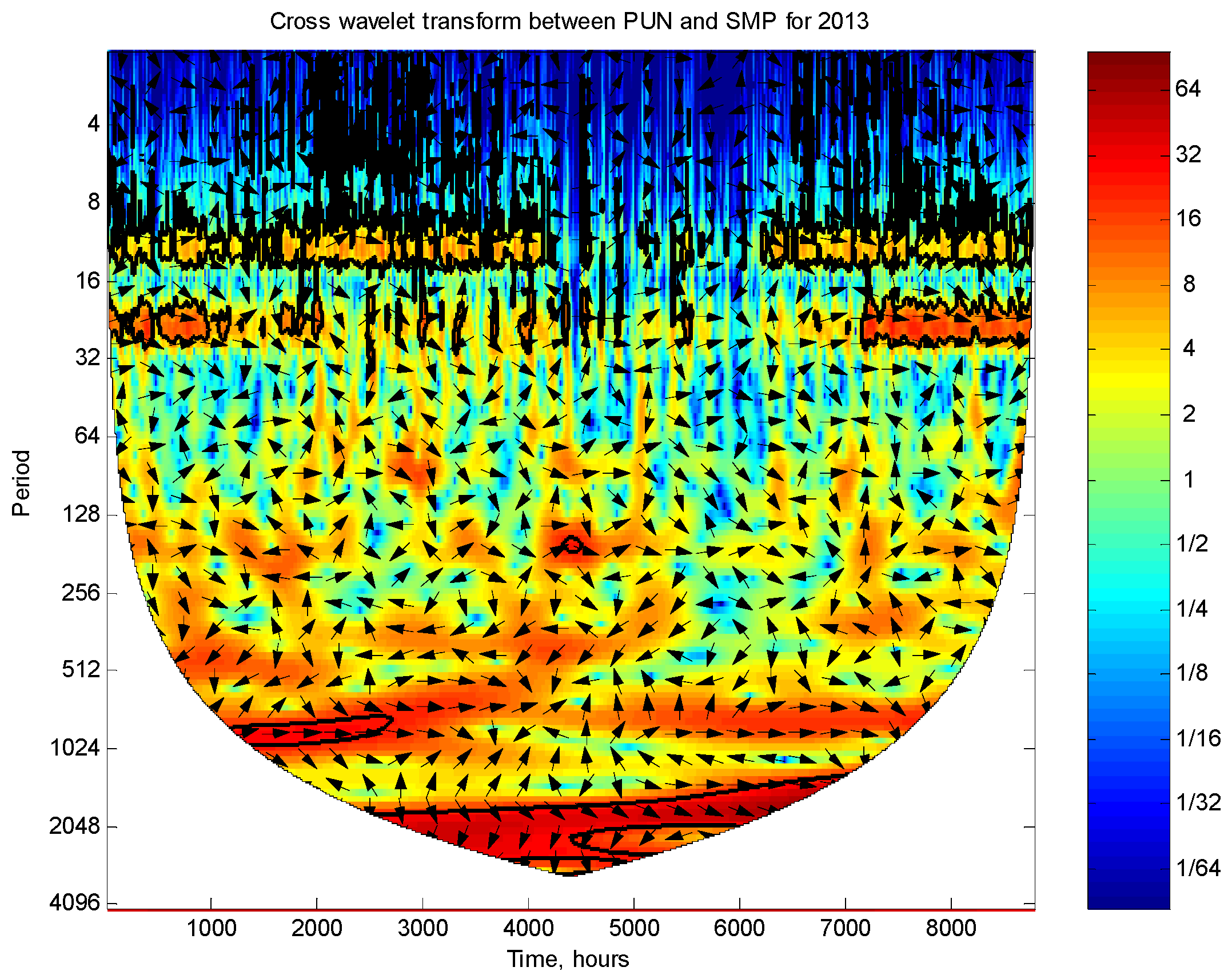
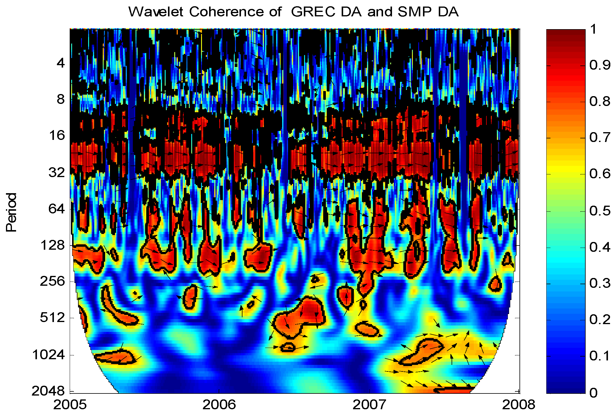
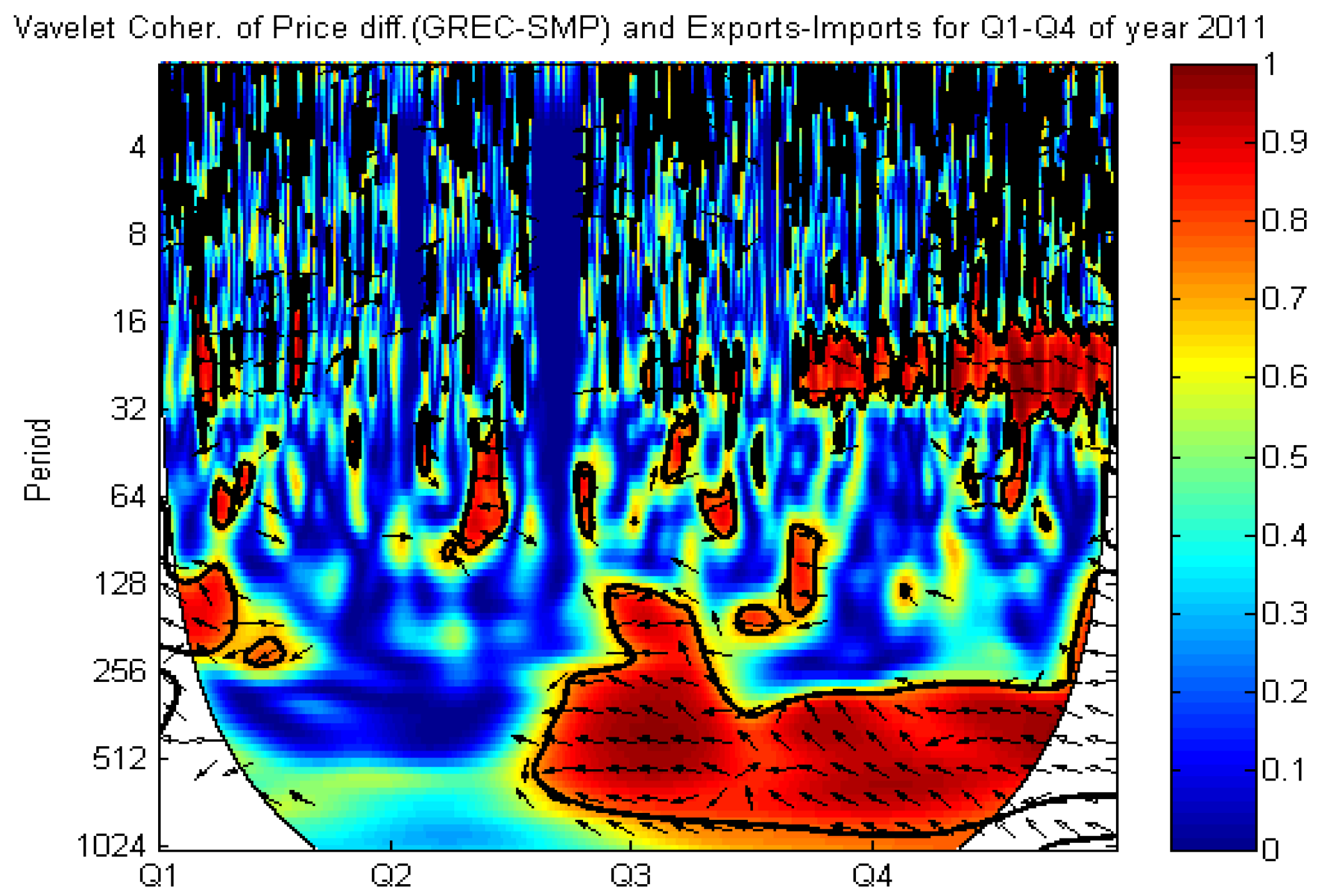
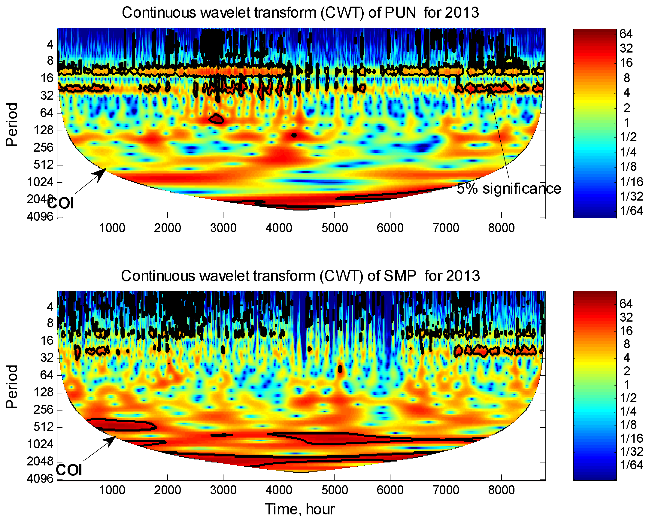
3.2. Evidence from the Wavelet Coherence

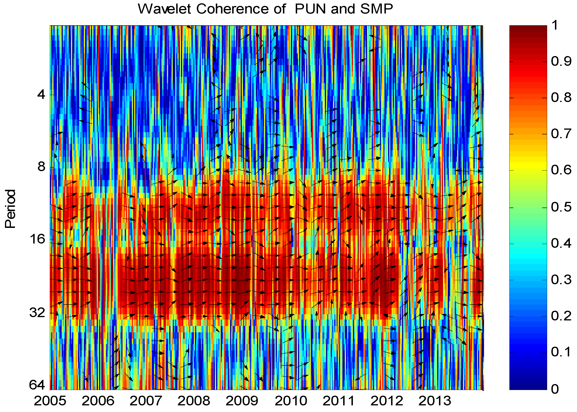
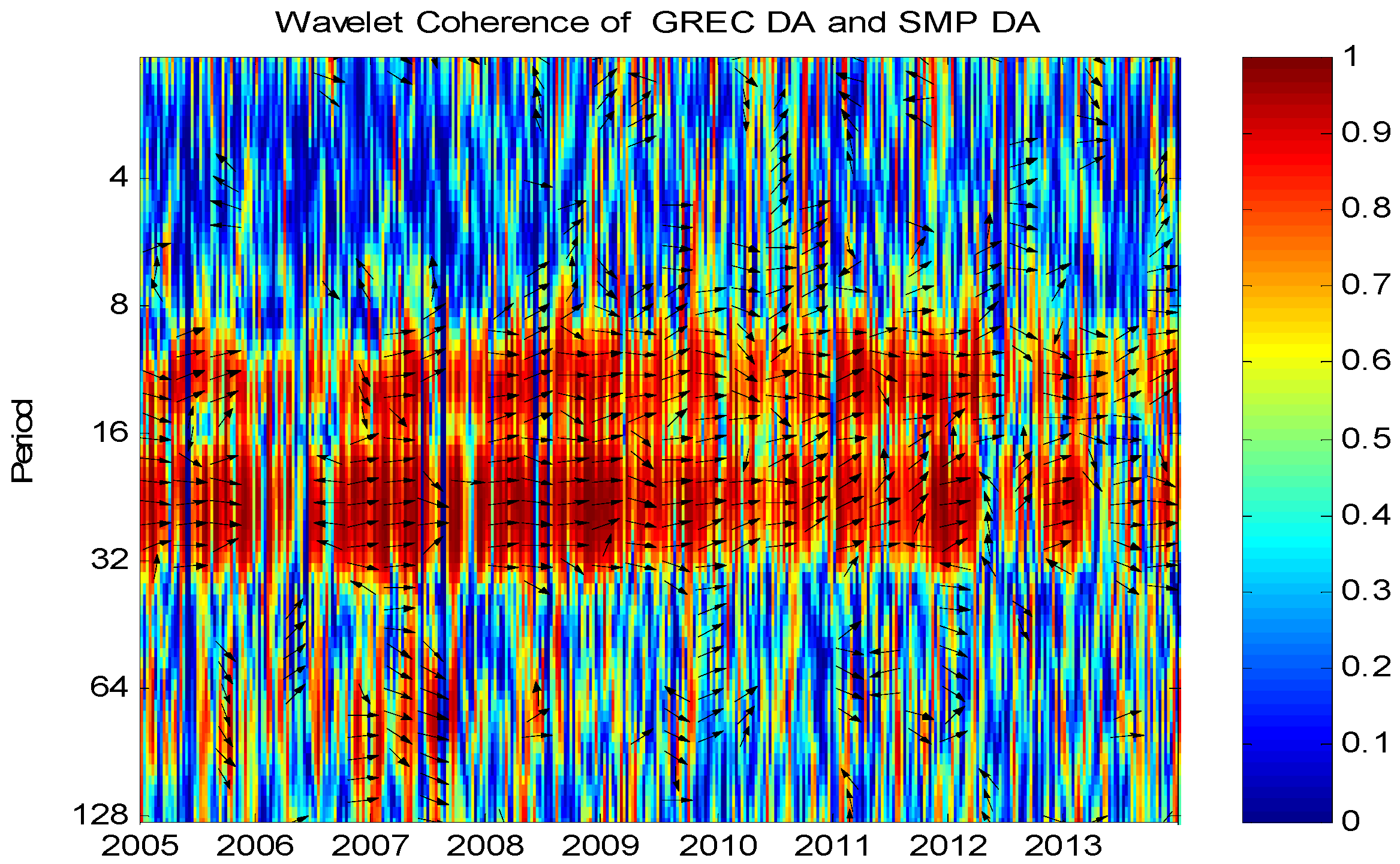
In energy commodities, an evidence of their strong inter-dependency is given by their unconditional correlations. It would be interesting however to study the time evolution of the correlations, given that data cover an extensive period of time. How these correlations depend on various frequencies? Are there any differences in the dependencies of two commodities when they are examined on different timeframe (long or short time windows)? Answers to these questions can be easily given by using the wavelet coherence methodology. Monte Carlo simulations will be used to assess the statistical significance of the estimated local correlations in the time frequency space.

Before we proceed to the CTW, XWT and WCT analysis of the time series in question, we must first be sure that an AR (1) noise process, as described in Section 2 (Equation (11)), is an appropriate null hypothesis. If the theoretical AR (1) spectrum is “a good model” for the power decay in the observed spectrum of say PUN, SMP etc., then this is usually an appropriate null hypothesis. We simply compare the two power spectra. To do this we estimate the power spectrum of the signals, using for example Burg’s algorithm. Then we fit our time series on an AR (1) model and obtain the lag autocorrelation coefficient, α. The previously estimated frequencies from the power spectrum of the time series, and the estimated α are the inputs in estimating the theoretical spectrum. These two spectra are then compared visually as to what degree the decaying behaviors of the two power spectra are similar. Figure 9 shows the results for the PUN and AR (1) decaying behaviors. The similarity is well pronounced so the AR (1) is accepted as an appropriate model for the null hypothesis.

In Figure 10 we show the continuous wavelet power spectrum of the PUN and SMP time series for the year 2013. The thick black contours designate the 5% significance level against red noise and the cone of influence, COI, where edge effects might distort the picture is shown as a white region. We observe that PUN and SMP exhibit similar, time dynamic behaviour, with “islands” of significant power at the same hour band (period) (12 and 24 h) and time (time spans within the year), with the “islands” more extended and continuous in the case of PUN. A similar to PUN behaviour is observed in GREC time series (not shown here). Therefore, we can choose PUN in our coherence as well as all other tests to follow, without any risk in our estimations of the degree of interdependence between the two markets.

Figure 9. The theoretical Fourier Power spectrum of an AR (1) process, with lag-1 autocorrelation a = 0.86 (estimated by fitting an AR (1) model on the observed PUN hourly time series for 2013, as given by relation Equation (11)) and the Power spectrum of the PUN time series 2013 estimated by a typical Burg’s algorithm. The two curves, decay with almost the same behaviour.

Figure 9. The theoretical Fourier Power spectrum of an AR (1) process, with lag-1 autocorrelation a = 0.86 (estimated by fitting an AR (1) model on the observed PUN hourly time series for 2013, as given by relation Equation (11)) and the Power spectrum of the PUN time series 2013 estimated by a typical Burg’s algorithm. The two curves, decay with almost the same behaviour.

Figure 10. The continuous wavelet power spectrum of the PUN and SMP time series for 2013. The thick black contours designate the 5% significance level against red noise and the cone of influence, COI, where edge effects might distort the picture is shown as a white region. The AR (1) lag-1 coefficients are 0.86 and 0.82 for PUN and SMP respectively.

Figure 10. The continuous wavelet power spectrum of the PUN and SMP time series for 2013. The thick black contours designate the 5% significance level against red noise and the cone of influence, COI, where edge effects might distort the picture is shown as a white region. The AR (1) lag-1 coefficients are 0.86 and 0.82 for PUN and SMP respectively.

The cross wavelet transform of PUN and SMP is shown in Figure 11. There are clearly common features in the wavelet power of the two prices, such as significant peaks in the 12 h band (period or scale) from the beginning of the year up to 4300 h (170 days or 6 months) band, then it follows a gap of no significant peak and finally, another “island” of significant peaks from the 6000 h band (i.e., the 9th month, September) to the end of year. So in June and July 2013 PUN and SMP do not show any common features in this hour band. The gap is due to the outage of cable after October virtual trade Greece-Italy and reduced capacity.

At the 24 h band we observe also two, shorter than before, time length “islands” of significance (high common power), the first of 1300 h’ time length or two months, corresponding to January and February and the other “island” of length of 1560 h, corresponding to the two last months of the year. The two series exhibit also significant power in the 768 h band (almost one month) and 2048 h band (~3 months). In the first, there is an “island” of significant peaks starting on February and ending on April 2013. An even larger significant “island” is in the 2048 h (~3 months) band, starting on April and ending in October (7200 h or 10 months).

In these two last “islands” of significant power, the relative phase relationship of PUN and SMP is that they are clearly in-phase (arrows pointing right) in the first region, while in the other, the situation is more complicated since some arrows are pointing right, others left (anti-phase) as well as down, reflecting the fact that SMP is leading PUN by 90°.

Especially in the 768 h band, the in-phase relationship between PUN and SMP could reveal important attributes towards the future Market Coupling between Greece and Italy.

Figure 11. Cross wavelet transform (XWT) of the PUN and SMP for 2013. The 5% significance level against red noise is shown as thick contour. The relative phase relationship is shown as arrows (with in-phase pointing right, anti-phased pointing left and SMP leading PUN by 90° pointing straight down.

Figure 11. Cross wavelet transform (XWT) of the PUN and SMP for 2013. The 5% significance level against red noise is shown as thick contour. The relative phase relationship is shown as arrows (with in-phase pointing right, anti-phased pointing left and SMP leading PUN by 90° pointing straight down.

In Figure 12 and Figure 13 we show the estimated wavelet coherence and the phase difference between PUN and SMP, and GREC and SMP, respectively, from scale (period) one hour band up to a scale of 64 h (to secure capturing daily dependence). On the horizontal axis of the figure is time, and on the vertical the scale or frequency; the lower the frequency, the higher the scale. The wavelet coherence, WC, tool detects the time-frequency regions where PUN and SMP co-evolve. Warmer colours (e.g., hot red) represent regions with significant dependence and they are enclosed by thick black lines contours. The colder the colour is, the less correlated PUN and SMP are. Regions where there is no dependence are outside the significant ones; therefore we can easily distinguish, both in time and frequency, the regions where the two prices co-move strongly. However, areas at the start and end of the examined time interval should be examined carefully, due to the inherent pathology of WC (as all similar transformation approaches share) the so-called edge effects. The cone of influence (COI), introduced earlier, takes care of this problem. COI is the region of the wavelet spectrum in which edge effects become important and is defined, as we have said, as the e-folding time for the autocorrelation of wavelet power at each scale (Torrence, C., et al., [29]).

From Figure 12 and Figure 13, we observe, as it is expected, that prices have a strong Coherence in the range of 12 h band to 24 h (1day) band, and that this happens for the entire time length of 2005–2013. However, as we will see below, when we have a closer look at smaller time lengths (zooming), say of 3 years or even smaller (of one year) duration, we find very interesting structures of strong interdependence and regions with large gaps where nothing happens (deep blue regions).

In both figures, for the range of scale 32 to 128 h and for entire time span of our series (2005–2013), there seems to be no or extremely weak dependence (the blue colour range from 0.1 to 0.3, indicating extremely low degree of correlation), though we see some sporadic hot regions as in 2007, 2008. The arrows in the hot regions and for most of the time span are heading to the right and some right-upward or right-downward. According to the explanation given in Section 2, GREC and SMP are in-phase. Also in cases where arrows point downward GREC is leading SMP 90°, while for the upward pointing arrows it happens the opposite.

Figure 12. Wavelet coherence of hourly price PUN and SMP DA. The horizontal axis shows time, while the vertical axis shows the scale or period in hours. The warmer the colour of a region, the higher the degree of dependence or coherence between the two series.

Figure 12. Wavelet coherence of hourly price PUN and SMP DA. The horizontal axis shows time, while the vertical axis shows the scale or period in hours. The warmer the colour of a region, the higher the degree of dependence or coherence between the two series.

We now proceed to examining the wavelet coherence in smaller time spans. In Figure 14 we expand time scale (zooming) from 2005 to 2007, so we can see details of the correlation structure that can’t be detected from Figure 12 and Figure 13.

Figure 13. Wavelet coherence of hourly price GREC DA and SMP DA. The horizontal axis shows time, while the vertical axis shows the scale or period in hours. The warmer the colour of a region, the higher the degree of dependence or coherence between the two series.

Figure 13. Wavelet coherence of hourly price GREC DA and SMP DA. The horizontal axis shows time, while the vertical axis shows the scale or period in hours. The warmer the colour of a region, the higher the degree of dependence or coherence between the two series.

Figure 14. Wavelet coherence of GREC and SMP for period 2005–2007. The horizontal axis shows time, while the vertical axis shows the scale or period in hours. The warmer the colour of a region, the higher the degree of dependence or coherence between the two series.

Figure 14. Wavelet coherence of GREC and SMP for period 2005–2007. The horizontal axis shows time, while the vertical axis shows the scale or period in hours. The warmer the colour of a region, the higher the degree of dependence or coherence between the two series.

In Figure 14 and Figure 15, all hot red “islands” of strong co-movement, inside a predominantly blue and yellow-green “sea” with arrows pointing in the left direction, are emerging in periods where mainly wrong flows are predominant. The left direction of the arrows shown on the graphs of Wavelet Coherence analysis, for the hot red areas defined by the “borders” set horizontally by the range of time starting final quarter of 2007 to the beginning of 2008 and vertically by the range of period or scale 8 to 32 h and the final half of 2011 to the beginning of 2012 and vertically by the range of period or scale 16 to 32 h and 256 (10 days) to 1024 h (40 days), are periods according to Table 4 where an increased amount of “wrong” flow is present. The arrows pointing to the left reflect that the price difference series is negatively correlated with the series Italy’s Net Exports (Exports from Italy-Imports to Italy) (or equivalently Imports of Greece-Exports of Greece) indicating “wrong” flows for Imports to Italy. Further examination of final half of 2011 to the beginning of 2012 and vertically by the range of period or scale 16 to 32 h and 256 (10 days) to 1024 h (40 days), shows that in many hours the SMP is increasing and remains larger than GREC, so the price difference is negative. Since GREC < SMP if flow of power is from Italy to Greece Exports (Exports from Italy-Imports to Italy) are negative, that is Imports to Italy are more than the Exports from Italy. This means that Price difference and Net Exports series are positively correlated and indicate a “wrong” flow.

Figure 15. Wavelet coherence of hourly price difference (GREC DA (Day Ahead)–SMP DA) and Exports-Imports difference, for the period 2011. The horizontal axis shows time in Quarters Q₁ to Q₄, while the vertical axis shows the scale or period in hours. The warmer the colour of a region, the higher the degree of dependence or coherence between the two series.

Figure 15. Wavelet coherence of hourly price difference (GREC DA (Day Ahead)–SMP DA) and Exports-Imports difference, for the period 2011. The horizontal axis shows time in Quarters Q₁ to Q₄, while the vertical axis shows the scale or period in hours. The warmer the colour of a region, the higher the degree of dependence or coherence between the two series.

Table 4. Clarification of Variable direction in relation with adverse and right flows.

Price Difference GREG-SMP	ITALY’s NET Exports Exports-Imports
	Wrong Flow	Right Flow
+ (>0)	+ (>0)	− (<0)
− (<0)	− (<0)	+ (>0)
Arrow Direction	←	→

Table 4. Clarification of Variable direction in relation with adverse and right flows.

Price Difference GREG-SMP	ITALY’s NET Exports Exports-Imports
	Wrong Flow	Right Flow
+ (>0)	+ (>0)	− (<0)
− (<0)	− (<0)	+ (>0)
Arrow Direction	←	→

In Figure 12, Figure 13, Figure 14 and Figure 15 above, the arrows pointing to the left reflect that the price difference series is negatively correlated with the series Italy’s Net Exports. If SMP is increasing and remains larger than GREC, then the price difference is negative. Since GREC < SMP the flow of power must be from Italy to Greece so it is expected that on pure commercial reasons, the Exports from Italy must be larger than Imports to Italy, therefore Net Exports must be a positive quantity. This means that Price difference and Net Exports series are positively correlated, as it is correctly shown by the right direction of the arrows shown on the graph, for example in the hot red (high degree of dependence or co-movement) area defined by the “borders” set horizontally by the range of time final quarter of 2011—beginning of 2012 and vertically by the range of period or scale 8 to 32 h). On the top and bottom of this area just described, there are two areas of very weak to almost negligible co-movement, defined vertically by scales 1 to 8 h and 32 to 256 h and horizontally by time 1st quarter of 2006 to end of 2013. Areas occupied with upward and left moving arrows, indicate that Price difference leads Net exports by 90° and is negatively correlated to it. The composite areas shown in the above figures, form “islands” of high and variable co-movement of the two series, both in time and scale (frequency) that detects correctly the right or wrong flow of power from one country to the other. This information, i.e., the variation of the co-movement simultaneously on time-frequency domain, however, can’t be obtained from using traditional tools (see, for example, in Section 3.3), enhancing our view that the Wavelet Coherence has a competitive advantage over other tools. To complete our comments on the figure, we say that all hot red “islands” of strong co-movement, inside a predominantly blue and yellow-green “sea”, occupied by arrows heading left, right, up and down, have a similar explanation and provide extremely useful and unique information about the right and wrong power flow directions that are in accordance with the overall co-movement of the two markets.

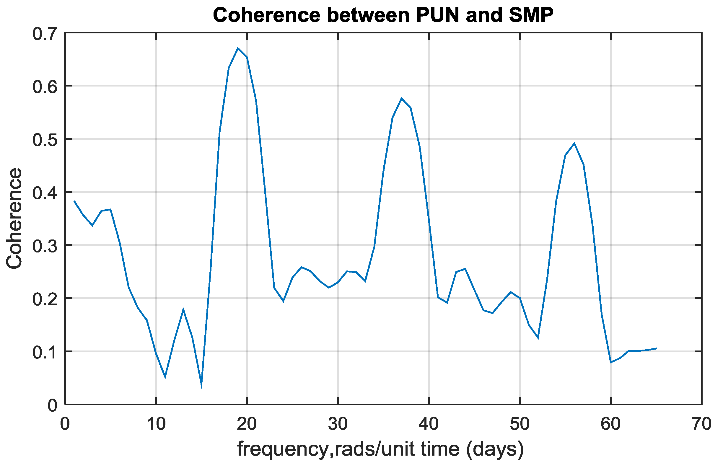
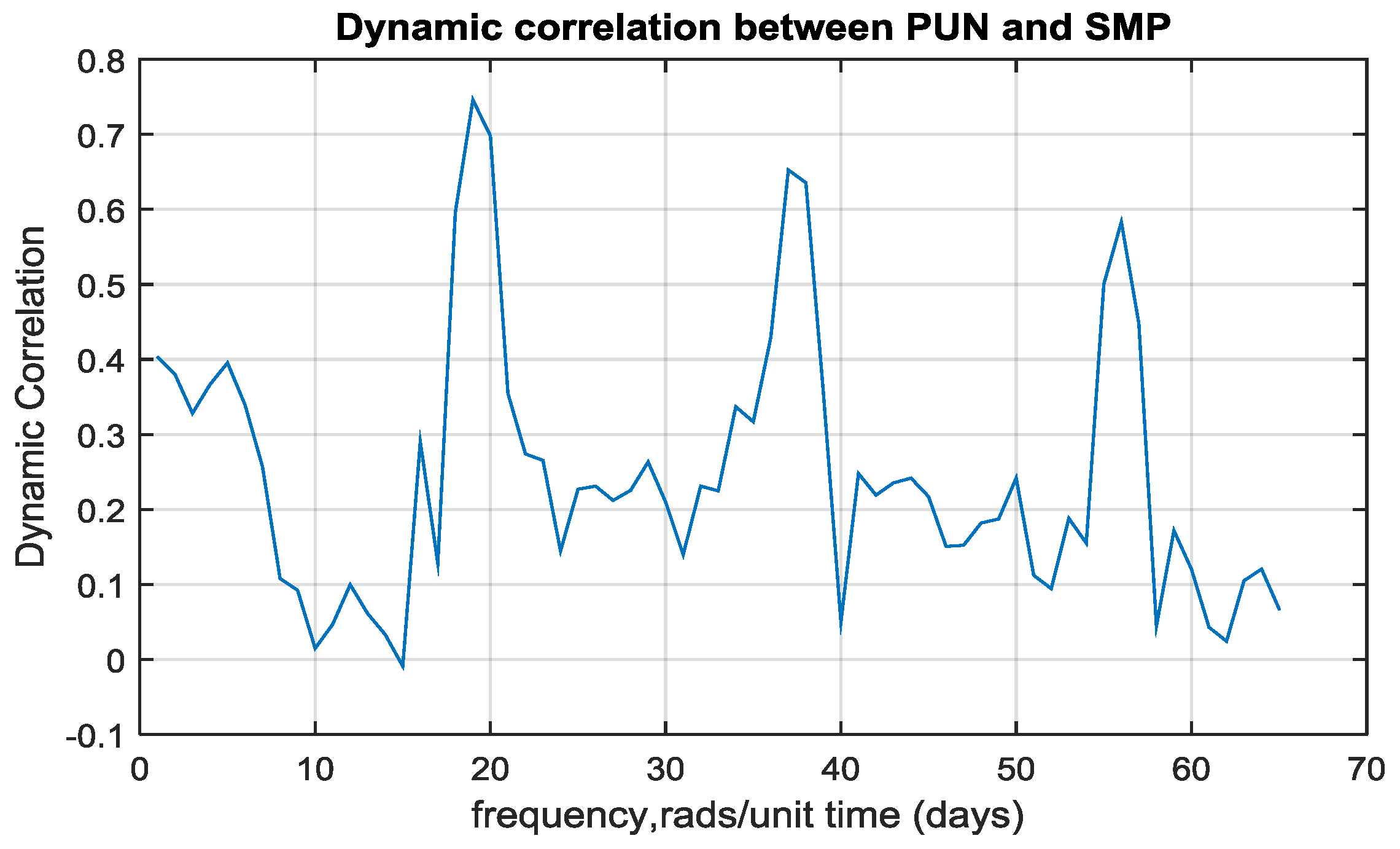
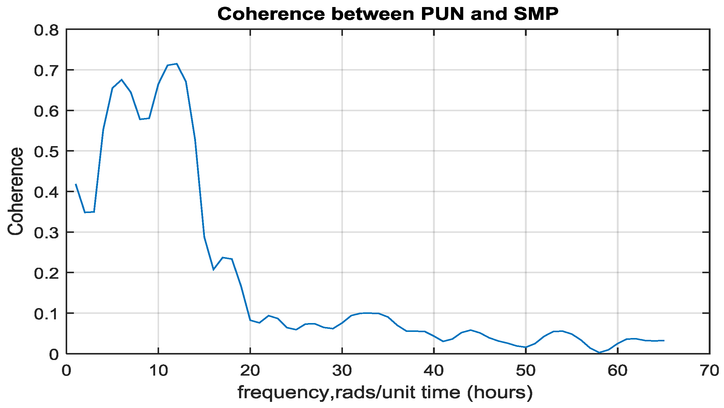
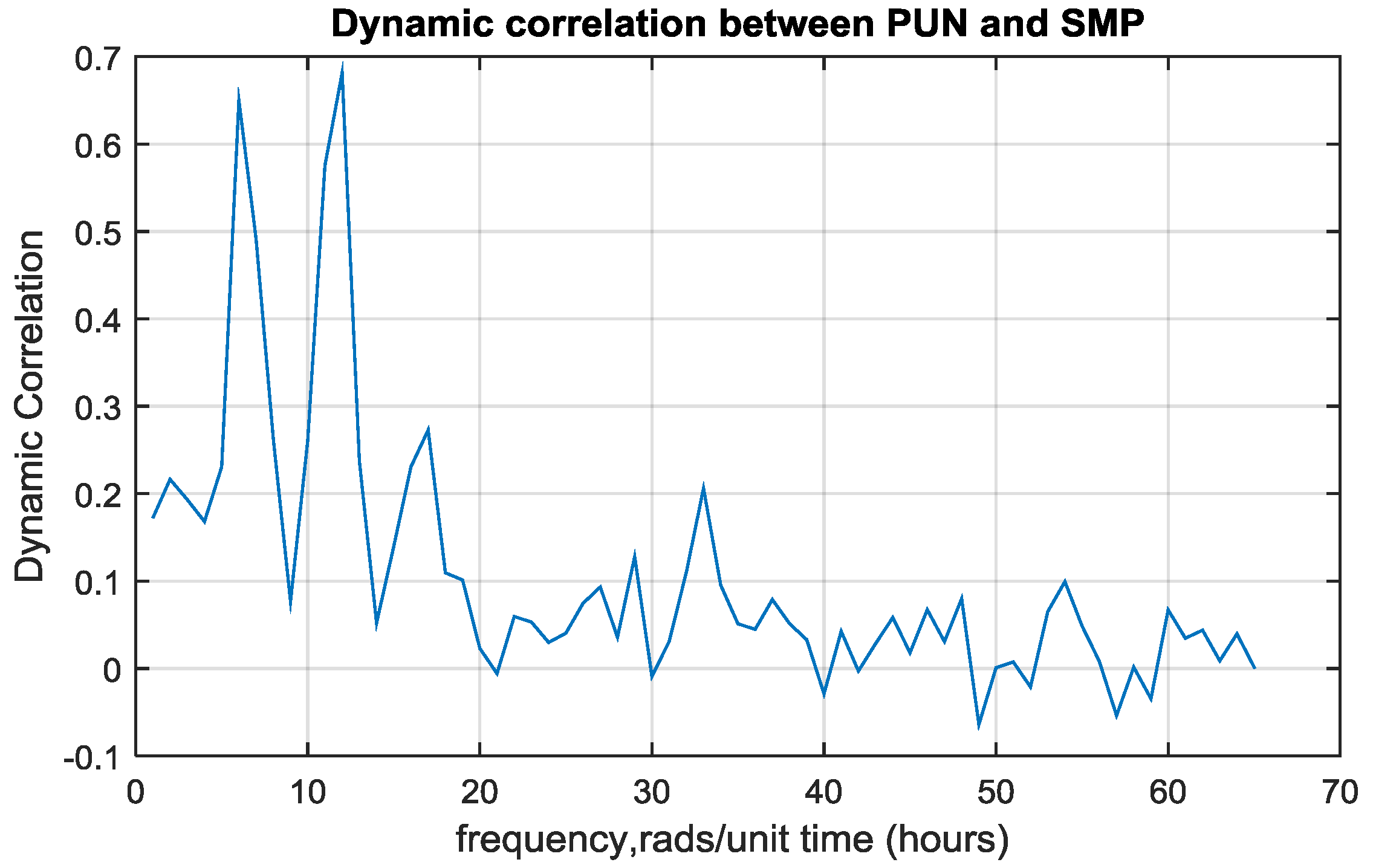
3.3. Evidence from Dynamic Correlation and Coherence Analysis

In addition to continuous wavelet coherence analysis we applied two, more traditional, spectral regression methods to the SMP and PUN indexes; namely coherence and dynamic correlation, an approach that has been applied to Macroeconomic time series in studying business cycle synchronization [35]. The outcome of these methods further validates the results of the wavelet coherence analysis. Additionally, since we utilize three distinct computational tools, we take advantage of the opportunity to compare the efficiency of the methods.

Based on the plateau that extends from one to six days as it is shown in Figure 16, which has been drawn by using the coherence approach of Section 3.2., we can conclude that the two time series have short term interdependence. The most prominent feature of the plot however is the spike at the nineteen days frequency. This indicates that the two market prices are strongly interdepended over that range. The subsequent coherence spikes that appear at integer multiples of nineteen days are harmonics of the latter dependence, indicating that the relationship between the SMP and the PUN is not sinusoidal.

Figure 16. Coherence plot between the SMP and PUN daily series, after applying relation Equation (13), Section 3.2.

Figure 16. Coherence plot between the SMP and PUN daily series, after applying relation Equation (13), Section 3.2.

In Figure 17 we show the evolution of ρ_xy between PUN and SMP daily series (relation Equation (14)). We come across the same striking features that appear in Figure 16. This is expected, due to the similar forms of Equations (13) and (14). Additionally, since the coherence series c_xy(f) is positive over the entire period examined we can deduce that one signal steadily leads the other, over the corresponding frequency band.

Figure 17. Dynamic correlation between the SMP and PUN daily time series, after applying relation Equation (14), Section 3.2.

Figure 17. Dynamic correlation between the SMP and PUN daily time series, after applying relation Equation (14), Section 3.2.

We now repeat the calculations for coherence and dynamic correlation between the SMP and PUN regarding now hourly data.

Both Figure 18 and Figure 19 provide further evidence of strong dependence between the two prices over the two frequency bands, centred on six and twelve hours respectively. These findings are in agreement with the wavelet coherence plots (Figure 12, Figure 13, Figure 14 and Figure 15), in which we can clearly observe two distinct red coloured ribbons over the same frequency bands.

Figure 12, Figure 13, Figure 14 and Figure 15 clearly reveal the advantages of continuous wavelet coherence over the traditional co-movement analysis methods [14]. Coherence and dynamic correlation graphs indicate interdependencies over specific frequency ranges. It should be noted however that they do not provide us with any information regarding the intensity of the interdependencies over time. In contrast, continuous wavelet analysis clearly depicts the impact of all frequency bands during each sample.

Specifically, in Figure 12 we can see that, for a short time period immediately after 2006, the six and twelve hour interdependencies were significantly diminished. This information cannot be obtained by observing Figure 18 or Figure 19. In this sense wavelet coherence analysis provides us with more succinct findings than conventional methods. Coherence and dynamic correlation provide us with a metric of the averaged impact of each frequency band over the entirety of the sample, however obscuring the time-specific relation of the signals.

Figure 18. Coherence plot between the SMP and PUN hourly prices.

Figure 18. Coherence plot between the SMP and PUN hourly prices.

Figure 19. Dynamic correlation plot between the SMP and PUN hourly prices.

Figure 19. Dynamic correlation plot between the SMP and PUN hourly prices.

4. Conclusions

In this work we have analyzed, in frequency and time domains, the cross border electricity trade between Greece and Italy, for the period 2005–2013, during which this interconnection trade has gradually transformed from a mere, traditional product of a state monopoly (the Greek side) to a more contemporary, multiple agent participation and liberalized energy commodity.

In the analysis we have used three different methods in detecting dynamic correlation or co-movement between two time series, in our case between PUN, GREC and SMP wholesale electricity prices. More specifically, we used the traditional approaches of dynamic correlation and cohesion that provide information on these two behaviors in time (but not simultaneously in frequency) and the contemporary wavelet method that provides information, in time-frequency space, about the co-movement of two signals. This later approach was applied on PUN, GREC and SMP prices as well as on the series of differences of PUN-SMP or GREC-SMP and Exports-Imports to produce a number of extremely useful plots as Continuous Wavelet Transform (CWT), Wavelet Coherence (WC), etc. in order to measure the intensity of dynamic local correlation between the two electricity markets, as well as the direction of (“right” and “wrong”) power flows in the interconnection. Wavelet analysis in our case has revealed significant information of how these two markets have co-evolve over the period of 2005–2013, both in time and frequency, revealing as well how the various regulatory reforms in Greece and Italy as well as how the critical technical events (e.g., outages, failures) in the interconnection have all influenced (in time and frequency) the trading of Power between these two Countries. In the analysis the superiority of Wavelet approach, in comparison with the other two methods, has become apparent, due to the fact that has provided information on the complexity of the interdependence of the two markets that is not possible to be extracted by the other two methods.

The results of this analysis, as described in details in the sections of this work, can be useful, as the authors believe, in understanding better the dynamics of the co-evolution of the power flow between Italy and Greece, especially now that the Greek market is about to be “coupled” with the Italian market, within the framework of the European Target Model.

The results of the analysis of the dynamics of co-movement of System Marginal Prices of Greek and Italian electricity markets presented in this work, is an important information in the process of preparing the coupling of the two Markets. In this paper, continuous wavelet analysis employed to assess the strength of the co-movement. This methodology allows for the examination of time-and-frequency varying co-movement within a unified framework. The importance of wavelet analysis reveals both short and long run dynamics of price co-movements, providing valuable information for policy makers (Regulators, TSOs, Market Operators), because, through wavelet coherency and phase-difference analysis, we can extract information on how time-frequency effects of price changes in one country (say Italy) can have an impact on the cross-border trading between the two interconnected countries.

We have seen that the strength of co-movement varies considerably across the two markets, at different frequencies (time horizons) and over time. In addition, we have seen that in some periods of time, in 2005-2013, the co-movement is stronger at lower frequencies (longer horizons) and increases during or just after periods characterized of strong regulatory or operational changes in the two markets.

A further policy implication of the findings of this work is described as follows.

The strengthening of efforts towards a European electricity market coupling (European Target Model, ETM), has gradually transform cross-border trading out of a primarily operational into a more liquid market in which transactions are gradually becoming financial rather physical. This market coupling has considerable effect on the Physical as well as Financial Transmission Rights (PTR and FTR). More specifically, ETM has already change the Use-It-Or-Sell-It (UIOSI) feature of PTR therefore allowing longer-term PTRs (to benefit from increased hedge effectiveness) as well as the increase of FTR due to large interest of financial players. In general, ETM have resulted in more competitive bids for PTRs the valuation of which is done via the traditional spread option approach.

After joining ETM, the Greek electricity market will has access to a plethora of PTRs and various FTRs instruments. A crucial parameter in the valuation of these instruments is their time horizon or maturity of the contract. Also, an ability to “forecast” in time (and frequency) the evolution of the spot electricity price is also very important. In this paper, via wavelet analysis, we have the ability to identify distinct time-frequency horizons of strong explanatory power in understanding the dynamics of co-movement of the two electricity markets. This valuable information can be used by policy makers in designing the coupling of Greek and Italian markets for a “smooth” introduction of PTRs, FTRs and the associated hedging opportunities, especially in the Greek market.

References

1. Regulation (EC) No 714/2009. In Proceedings of the European Parliament and the Council on the conditions for access to the network for cross-border exchanges in electricity and repealing Regulation (EC), Regulation of European Parliament and of the Council, Brussels, Belgium, 13 July 2009.
2. Bunn, D.W. Modelling in Competitive Electricity Markets; Wiley: New York, NY, USA, 2004; pp. 1–17. [Google Scholar]
3. Hong, Y.; Wu, C.P. Day-ahead electricity price forecasting using a hybrid principal component analysis network. Energies 2012, 5, 4711–4725. [Google Scholar] [CrossRef]
4. Aguiar-Conraria, L.; Azevedo, N.; Soares, M.J. Using wavelets to decompose the time frequency effects of monetary policy. Physica A 2008, 387, 2863–2878. [Google Scholar] [CrossRef] [Green Version]
5. Ramsay, J.B. Wavelets in economics and finance: Past and future. Stud. Nonlinear Dyn. Econ. 2002, 6. [Google Scholar] [CrossRef]
6. Voronin, S.; Partanen, J. price forecasting in the day-ahead energy market by an iterative method with separate normal price and price spike frameworks. Energies 2013, 6, 5897–5920. [Google Scholar] [CrossRef]
7. Naccache, T. Oil price cycles and wavelets. Energy Econ. 2011, 33, 338–352. [Google Scholar] [CrossRef]
8. Tan, Z.; Zhang, J.; Wang, J.; Xu, J. Day-ahead electricity price forecasting using wavelet transform combined with ARIMA and GARCH models. Appl. Energy 2010, 87, 3606–3610. [Google Scholar] [CrossRef]
9. Connor, J.; Rossiter, R. Wavelet transforms and commodity prices. Stud. Nonlinear Dyn. Econ. 2005, 9. [Google Scholar] [CrossRef]
10. Yousefi, S.; Weinreich, I.; Reinarz, D. Wavelet-based prediction of oil prices. Chaos Solut. Fractals 2005, 25, 265–275. [Google Scholar] [CrossRef]
11. Davidson, R.; Labys, W.C.; Lesourd, J. Wavelet analysis of commodity price behaviour. Comput. Econ. 1997, 11, 103–128. [Google Scholar] [CrossRef]
12. Ghoshray, A.; Johnson, B. Trends in world energy prices. Energy Econ. 2010, 32, 1147–1156. [Google Scholar] [CrossRef]
13. Grine, S.; Diko, P. Multi-layer model of correlated energy prices. J. Comput. Appl. Math. 2010, 233, 2590–2610. [Google Scholar] [CrossRef]
14. Ciarreta, A.; Zarraga, A. Analysis of volatility transmissions in integrated and interconnected markets: The case of the Iberian and French markets. Document. Trabajo Biltoki 2012, 4, 1–25. [Google Scholar]
15. Bunn, D.; Zachmann, G. Inefficient arbitrage in inter-regional electricity transmission. J. Regul. Econ. 2010, 37, 243–265. [Google Scholar] [CrossRef]
16. Boffa, F.; Sapio, A. Introduction to the special issue “The Regional Integration of Energy Markets”. Energy Policy 2015, 85, 421–425. [Google Scholar] [CrossRef]
17. McInerney, C.; Bunn, D. Valuation anomalies for interconnector transmission rights. Energy Policy 2015, 55, 565–578. [Google Scholar] [CrossRef]
18. Boffa, F.; Scarpa, C. An anticompetitive effect of eliminating transport barriers in network markets. Rev. Ind. Organ. 2009, 34, 115–133. [Google Scholar] [CrossRef]
19. Fuss, R.; Mahringer, S.; Prokopczuk, M. Market Coupling in Electricity Markets: Status quo and Future Challenges. Available online: http://papers.ssrn.com/sol3/Papers.cfm?abstract_id=2509239 (accessed on 13 October 2015).
20. Mallat, S.G. A theory for multiresolation signal decomposition: the wavelet representation. IEEE Trans. Pattern Anal. Mach. Intell. 1989, 11, 674–693. [Google Scholar] [CrossRef]
21. Gençay, R.; Selçuk, F.; Whitcher, B. An Introduction to Wavelets and Other Filtering Methods in Finance and Economics; Academic Press: London, UK, 2002. [Google Scholar]
22. Warner, R.M. Spectral Analysis of Time-Series Data; The Guildford Press: New York, NY, USA, 1998. [Google Scholar]
23. Percival, D.; Walden, A. Wavelet Methods for Time Series Analysis; Cambridge University Press: Cambridge, UK, 2000. [Google Scholar]
24. Bruce, A.; Gao, H. Applied Wavelet Analysis with S-Plus; Springer-Verlag: Berlin, Germany, 1996. [Google Scholar]
25. Adisson, P. The Illustrated Wavelet Transform Handbook; The Institute of Physics: London, UK, 2002. [Google Scholar]
26. Grinsted, A.; Moore, J.C.; Jevrejeva, S. Application of the cross wavelet transform and wavelet coherence to geophysical time series. Nonlinear Process. Geophys. 2004, 11, 561–566. [Google Scholar] [CrossRef]
27. Rua, A.; Nunes, L.C. International co-movement of stock market returns: A wavelet analysis. J. Empir. Financ. 2009, 16, 632–639. [Google Scholar] [CrossRef]
28. Torrence, C.; Webster, P.J. Interdecadal changes in the ENSO-monsoon system. J. Clim. 1999, 12, 2679–2690. [Google Scholar] [CrossRef]
29. Torrence, C.; Compo, G. A practical guide to wavelet analysis. Bull. Am. Meteorol. Soc. 1998, 79, 61–78. [Google Scholar] [CrossRef]
30. Martina, E.; Rodriguez, E.; Escarela-Perez, R.; Alvarez-Ramirez, J. Multiscale entropy analysis of crude oil price dynamics. Energy Econ. 2011, 33, 936–947. [Google Scholar] [CrossRef]
31. Allen, M.R.; Smith, L.A. Monte Carlo SSA: Detecting irregular oscillations in the presence of coloured noise. J. Clim. 1996, 9, 3373–3404. [Google Scholar] [CrossRef]
32. Bollerslev, T. Modelling the coherence in short-run nominal exchange rates: A multivariate generalized arch model. Rev. Econ. Stat. 1990, 72, 498–505. [Google Scholar] [CrossRef]
33. Engle, R. Dynamic conditional correlation: A simple class of multivariate generalized autoregressive conditional heteroskedasticity models. J. Bus. Econ. Stat. 2002, 20, 339–350. [Google Scholar] [CrossRef]
34. Lanza, A.; Manera, M.; McAleer, M. Modelling dynamic conditional correlations in WTI oil forward and futures returns. Financ. Res. Lett. 2006, 3, 114–132. [Google Scholar] [CrossRef]
35. Croux, C.; Forni, M.; Reichlin, L. A measure of co-movement for Economic variables: Theory and empirics. Rev. Econ. Stat. 2001. [Google Scholar] [CrossRef]
36. Annual Report on the Results of Monitoring the Internal Electricity and Natural Gas Markets in 2012. Agency for the Cooperation of Energy Regulators, ACER/CEER, 29 November 2012.
37. Papaioannou, G.P.; Papaioannou, P.G.; Parliaris, N. Modelling the Stylized Facts of the Wholesale System Marginal Price and the Impact of Regulatory Reforms on the Greek Electricity Market. Available online: http://arxiv.org/abs/1401.5452 (accessed on 13 October 2015).
38. Petrella, A.; Sapio, A. Assessing the impact of forward trading, retail liberalization and white certificates on the Italian wholesale electricity prices. Energy Policy 2012, 40, 307–317. [Google Scholar] [CrossRef]
39. Andrianesis, P.; Biskas, P.; Liberopoulos, G. An overview of Greece’s wholesale electricity market with emphasis on ancillary services. Electr. Power Syst. Res. 2011, 81, 1631–1642. [Google Scholar] [CrossRef]
40. Regulatory Authority for Energy (RAE). National Report to the European Commission, Athens, Greece, November 2010. Available online: http://www.rae.gr (accessed on 13 October 2015).
41. Di Cosmo, V. Modelling the Italian electricity price. In Proceedings of the Economic and Social Research Institute Trinity College, IEB Symposium, Dublin, Ireland, 20–23 August 2015.
42. Corrado, C.; Assanelli, M. An overview of Italy’s Energy Mix. Gouvern. Eur. Géopol. L’Énergie, June 2012. Available online: http://www.ifri.org (accessed on 13 October 2015).
43. Cataldi, A.; Stefano, C.; Zoppoli, P. The Merit-Order effect in the Italian power market: The Impact of solar and wind generation on national wholesale electricity prices. Energy Policy 2015, 77, 79–88. [Google Scholar]
44. Italian Power Exchange, IPEX. Available online: http://www.mercatoellettrico.org (accessed on 13 October 2015).
45. Greek Independent Power Transmission Operator, IPTO, ADMIE SA. Available online: http://www.admie.gr (accessed on 13 October 2015).