1. Introduction
The Optimal Power Flow (OPF) is a very important issue in power systems. For the operator, fixed generated power corresponds to one operating condition only. Optimized operation very often demands an adjustment of generation, as loads and renewable based generation vary, according to given objectives. Typical ones are minimization of power losses or minimization of production cost. The application of such criteria immediately implies variable generated power and relevant bus voltages, which have to be determined so that both or one of the two objectives is achieved. The problem [
1] is intrinsically complex and computationally expensive, the relevant optimization is nonlinear and nonconvex and may include both binary and continuous variables.
The formulation of OPF typically refers to a centralized approach, for which a processing unit solves the problem starting from measures collected from Intelligent Electronic Devices (IEDs) connected to apparatus of the power network. This centralized architecture can be found in power systems even at the distribution level and even in modern power distribution systems integrating a large amount of generated power form renewables, such as microgrids(MGs) [
2]. According to the United States Department of Energy, MGs can be defined as “localized grids that can disconnect from the traditional grid to operate autonomously and help mitigate grid disturbances to strengthen grid resilience…” they “… can play an important role in transforming the nation’s electric grid”… “MGs also support a flexible and efficient electric grid, by enabling the integration of growing deployments of renewable sources of energy such as solar and wind and distributed energy resources such as combined heat and power, energy storage, and demand response.”
Renewable sources of energy are typically inverter-interfaced units showing low inertia and causing regulation problems in power systems. In MGs, a three levels control hierarchical architecture [
3] allows to provide good power quality operation and more recently, experimental papers have been dealing with distributed secondary [
2], control, while practical distributed tertiary control for MGs and energy management is still under investigation [
4,
5].
OPF is essentially a tertiary level optimal operation issue in electric power systems and the latter has been for a long time a concern of many researchers. For this purpose, many optimization techniques have been used, such as “the steepest descent” method [
6], particle swarm optimization method [
7], Glow-worm Swarm Optimization (GSO) method [
8] fuzzy rules method [
9,
10], dynamic programming [
11], global optimization [
12,
13] and so forth. In addition, optimization problems have been solved considering the presence of energy storage systems, which are critical in islanded MGs systems [
10,
14,
15,
16,
17,
18,
19]. More recently, the authors in [
20] have proposed a solution, which combines the Lagrange method and Newton Trust Region method to solve centralized OPF in islanded microgrids in which generated power of generator and loads depend on frequency and voltage.
In the above mentioned research works, a form of central coordination is needed; they solve a centralized OPF problem and they need a centralized control system which shows disadvantages, such as low flexibility, low expandability and heavy computational burden. To cope with these disadvantages, decentralized OPF is a good idea and provides useful solutions especially for reconfigurable systems and plug-and-play applications. A distributed OPF approach has been first been proposed in [
21,
22] since 1997 to solve the OPF problem in transmission networks. In these two papers, the authors consider the OPF issue for sub-regions and coordinate the solution of multiple OPF problems through an iterative update on constraint Lagrange multipliers. Since then, the problem has been studied widely. In [
23], to solve the problem of decentralized OPF control, the authors have pursued an iterative approach delivered with a preconditioned conjugate gradient method. However, in this approach the management is highly centralized and it is addressed to power transmission systems. Also for power transmission systems, in [
24,
25] a similar incremental approach was presented, extended to solve the problem DC-OPF.
The authors in [
4] combined and broadened the approaches of [
21,
22] to unbalanced systems and employed the Alternating Direction Method of Multipliers (ADMM) to solve the problem of distributed OPF in unbalanced smart microgrids systems, but the method still requires the identification of sub-networks and is not fully decentralized; it also needs to solve the centralized problem and the approach seems very complex. In [
26], the ADMM was applied to solve OPF with an approach completely distributed/decentralized that do not need any form of central coordination. It was used a region-based optimization process where the exchanged information is limited only to neighboring regions. These approaches consider balanced transmission systems.
Finally, a decentralized approach employing a distributed reinforcement learning approach (distributed Q-learning) it is worth citing [
27]. This paper proposes a decentralized control algorithm to modify tap changers, capacitor banks and generation bus voltage in order to dispatch reactive power to reduce power losses. The paper applied distributed Q learning to a power dispatch problem in electrical power systems, but the approach does not consider the load flow solution thus needing continuous measurements of branch power flows to verify the quality of the implemented operating points, which do not seem easily applicable.
In this paper, we propose a simple distributed OPF algorithm in which an approximate solution of the OPF is reached without a central controller. Nodes exchange information only with its neighbors, and there is no need of information about the network’s topology. For this reason the proposed system is suitable also when switches reconfiguration takes place without any modification.
The required communication algorithm is simple, involving a lower communication overhead as compared to the centralized solutions; more robust against nodes and links failure, in fact we can add or remove nodes from the network and the algorithm will adapt to the new condition. In a centralized OPF, where loads and power appliances are accessible through the telecommunication network, the loss of control and operation of the power system’s apparatuses may seriously affect the real-time operation of the power system [
28].
The application on a small nine bus system is just a proof-of-concept of the proposed approach and is limited to active power generation correction. The application at this stage refers to a topology that is quite common in AC MGs in which an AC line supplies a set of loads; generators inject power in the same line but are physically located in different places according to how suitable the sites are for renewable energy generation.
Results are quite promising and suggest including reactive power generation correction to get to more precise solutions. Further studies will expand the considered solution approach to account for more complex topologies.
2. Scope of Work and Optimal Power Flow (OPF) Problem Formulation
With the basic hierarchical control architecture proposed in the literature for microgrids [
3], when a bus power injection suddenly varies (from a load or a generation source)
, the regulation process starts.
In this conventional control structure, three control levels can be evidenced:
- (1)
Primary control level for controlling local power, voltage and current. It typically follows the setting points given by upper level controllers and performs control actions over interface power conversion systems.
- (2)
Secondary control level appears on top of primary control. It deals with power quality control, such as voltage/frequency restoration, as well as voltage unbalance and harmonic compensation. In addition, it is in charge of synchronization and power exchange with the main grid or other MGs.
- (3)
Tertiary level introduces intelligence in the whole system. To that end, tertiary control will attempt to optimize the MG operation based on efficiency and/or economics, solving when necessary the OPF problem. Knowledge both from the MG side as well as the external main network is of utmost importance to execute the optimization functions and ICT (Information and Communication Technology) is a key technology for that issue. Local or centralized Decision-Making algorithms are employed to process the gathered information and take proper actions.
The bandwidth of communication channels of the different control levels are thus typically separated by at least one order of magnitude, implying the decoupling of the dynamics at different levels. This feature implies easier modelling and analysis of MGs systems. As we look at higher control levels, regulation speed becomes lower; e.g., droop control in primary level has typically a response within 1 to 10 ms, secondary control speed can get to 100ms up to 1s depending on the speed limit of the used communication technology, while tertiary control implements the actions in time steps ranging from seconds to hours.
While for primary and secondary levels, extensive literature provides decentralized implementation, a decentralized approach for tertiary regulation level is still under study. At this level, the solution of the OPF will produce a correction of the generators’ set points giving rise to minimum losses operation or minimum cost operation. In this paper, we focus on the identification of a sub-optimal minimum losses operation point using a distributed intelligence methodology.
The conventional OPF problem for power losses minimization can be formulated as follows. Consider a microgrid with N nodes, G of which are generators, including storage systems, and L of which are loads or non dispatchable renewable sources. The microgrid has B branches, for each of which the longitudinal electrical parameters can be indicated as Rk and Xk (where k = 1, … B).
The mathematical formulation of the centralized OPF problem can be written as follows:
where losses are determined solving a centralized load flow as follows:
under the following constraints:
where
Vi is the voltage module at the sending bus
i of branch
k;
i=
SB(
k).
respectively are the real and reactive power flows on branch k. respectively are the voltage module and its minimum and maximum rated values at bus i; respectively are the current flow module on the k-th branch and the k-th branch ampacity; respectively are the power injection at the i-thdispatchable generation node, its minimum and maximum values.
The optimization variables are the power injections at the generation buses, therefore Equation (1) must relate to these terms. In this paper, the methodology chosen for the solution of the OPF problem is heuristic. In this case, for centralized OPF the constraints can either be included in the objective function through penalty terms or can be considered afterwards, by discarding unfeasible solutions or by strongly penalizing them or even repairing them through heuristic repair methods. A decentralized formulation of the same problem is given in the following section, assuming that the overall energy balance of the microgrid does not change except for the limited amount of power losses that is minimized.
3. General Formulation and Methodology for Decentralized OPF
The methodology adopted in this paper to solve the decentralized OPF derives from the combination of approximated power flow algorithms like the well-known backward-forward [
29] algorithm and power flow tracing methods as discussed in [
30]. The idea is essentially to modify the power injected by the different sources that are installed in the microgrid, by applying the gradient descent method to reduce the power losses in each branch caused by each generator. The latter operation is carried out by calculating the partial derivatives of the power losses on each branch with respect to the contribution of power of the upstream generation source. Power losses on each branch can indeed be expressed as a function of the contribution to the power flow from each generator. Such assessment allows to correct the active power injected by each generation source. To understand if the correction has produced a variation of the voltages profile and thus to correctly evaluate the new power losses value, an on-line distributed power flow is also carried out.
The problem formulation thus becomes the following:
where losses are determined locally applying the Kirkhhoff current law at the sending and ending buses of the
k-th branch for which the sum of entering and outgoing flows on the adferent branches to a generic bus (
na in Equation (7)) must be zero:
Moreover, since the network is islanded, the corrections at the generators must have opposite signs so as to compensate the overall power balance.
The following constraints about voltages and currents will still hold at each generic bus
i and at each branch:
The following constraint about power generated from each source in the microgrid should also be considered:
To evaluate the correction to be executed on the generated power of each source minimizing the power losses on each branch, it is necessary to know to what extent the power flowing on a single branch can be attributed to a given source.
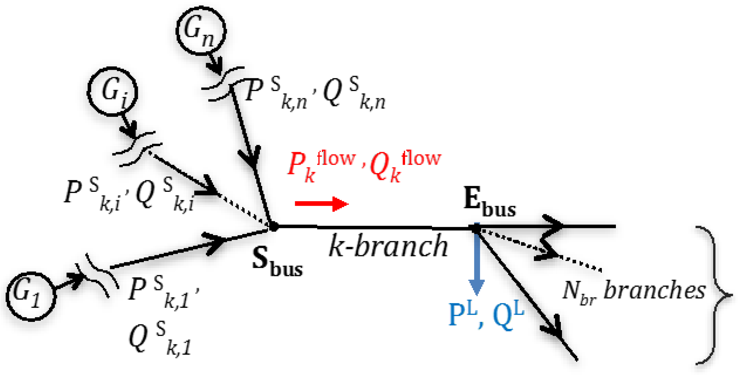
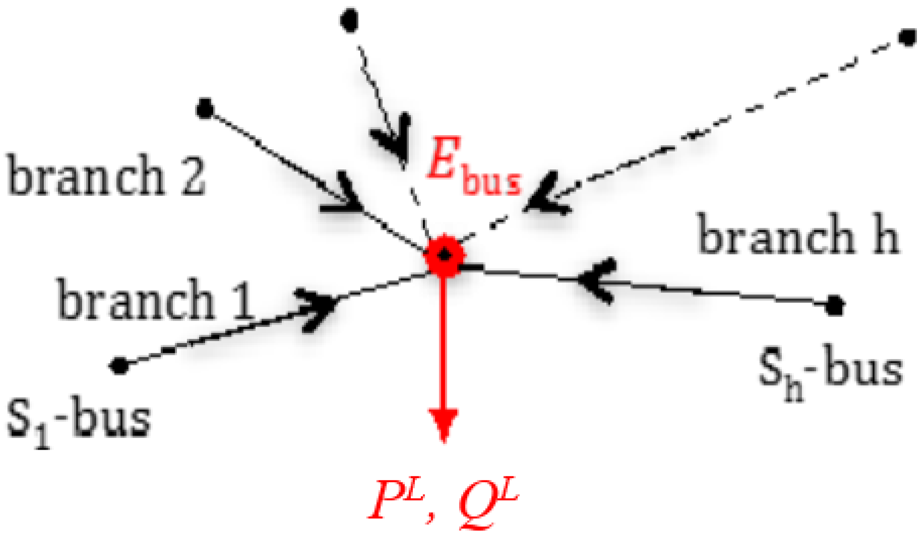
Referring to
Figure 1 below, Equation (11) shows the relation between the power flowing on branch
k, and the contribution of the generic
i-th generator (
Pk,iS;
Qk,iS) to the power flow in the same branch
k, under the hypothesis that the power flows from the sending bus
S to ending bus
E.
It can be argued that the contribution from a given source to the power flowing in branch k is proportional to the injected power from a generic generator.
In [
30], the authors study the problem of power losses partition and the following Equation (12) instead of Equation (6) can be used:
where the relation between the overall losses on branch
k,
ΔPk, and the contribution of the
i-th generator to the power flow in the same branch
k (
Pk,iS;
Qk,iS) is shown. In this expression,
Rk is the resistance of the
k-th branch and
VS is the voltage module at the sending bus. The same expression can be written, if reactive flows can be neglected, in the following way (see
Figure 1):
Under the hypothesis that power flows from the i-th generator in the generic branch k (Pk,iS; Qk,iS) can be somehow deduced, the minimization of Equation (13) allows to derive the active power correction that must be applied to the generated power according to the gradient method carried out only with respect to the active generated powers.
According to a heuristic rule, the partition of the flows in each branch among generators is at first determined and then adjusted along iterations, as it will be detailed later on in the paper.
Figure 1.
Partition of the power flows among generators in a generic branch k.
Figure 1.
Partition of the power flows among generators in a generic branch k.
To derive the terms (Pk,iS; Pk,jS) in Equation (13), it is necessary to solve the distributed load flow and contextually perform power flow tracing.
3.1. Distributed Power Flow
Distributed power flow is carried out according to the well-known backward/forward methodology described in [
29]. In this case, loads are modeled as constant power nodes and generators as constant power sources. To calculate the distributed load flow, it will be assumed that the following quantities are known because they can be locally measured:
voltage modules;
real and reactive power injected by generator buses;
real and reactive power absorbed by load nodes;
real and reactive power injected/absorbed by storage systems.
The only admitted communication is between adjacent nodes. The algorithm is divided in three parts: an initialization phase consisting in the power flow tracing starting from measured bus voltages collected on the grid. In this phase, each IED at each bus, at regular time intervals, measures the local voltage value and queries the neighboring nodes about bus voltage levels.
A second part, the backward phase, in which the IEDs at load nodes decide how to correct power generations; and finally a third step, the forward phase, in which the modification of the voltage profiles is carried out. From the updated voltage values, the power losses can be again calculated according to Equation (13). Backward and forward phases are repeated until convergence.
In what follows, a sink node is a load node with known real and reactive power (
PL,
QL) where the flows from the adjacent nodes converge; it is this a node showing the lowest voltage value as compared to the neighboring nodes, see node
E in
Figure 2.
Some basic concepts can be accounted for, in this process, when considering each generic branch
k:
- (1)
Loads are supplied through the adjacent branches in a proportion that probabilistically depends on the voltage level of adjacent buses.
- (2)
The power flow entering a branching node is shared among the outgoing branches following a heuristic sharing principle.
Figure 2.
A sink load node.
Figure 2.
A sink load node.
In this phase, constraints violations about currents (backward phase) and about voltages (forward phase) can be evidenced and the learning algorithm will account for it giving a negative feedback about the decided power correction.
3.2. Distributed Optimal Power Flow
To solve the OPF, the main step is to understand how the generators contribute to the power flow in each branch of the network. In the initialization phase, the voltage modules at each bus will tell the direction of the power flows in the branches at each step. In this way, the paths of the power supplied by generators are identified and the power inversion points are devised. As simplifying assumption, the real and reactive power inversion points are considered the same. In the same initialization phase, looking at the bus voltage levels, also the sink nodes can be identified.
In the backward phase starting from a sink node, when a correction to an upstream generator is decided on a given branch, the other generators power injections will have to be corrected in the opposite direction. In this way, the overall power balance is maintained, not considering the comparably low power losses. The paths in which the power generation correction is a decrement are first considered.
The method for corrections of active powers injected by the generators is the gradient descent method. Based on Equation (13) at each branch, partial derivatives, in each of the variables (
) of the power losses and in each branch will be calculated and these terms will be used to correct the generated power at the relevant source nodes. Once decided the amount of the power generation to be reduced in the considered path, the other paths are analyzed, evaluating how much increase each power generation unit must apply according to the power losses in the downstream paths. In
Section 4, this step is outlined in greater detail. This correction is to be applied at each iteration of the OPF procedure. Each iteration implies the visit of all nodes of the network.
The subsequent forward phase calculates the new bus voltages and weights of the learning procedure outlined below. The distributed OPF is carried out as described below through a backward/forward process starting from the sink nodes and following procedures listed below.
3.3. Backward Phase
Let’s first consider a generic sink bus
L supplied through
h branches (see
Figure 2). In order to proceed upwards, it is required to know how the load at bus
E in the figure must be divided into the adjacent upstream branches. This condition is expressed through the values of the α
k coefficients. These can be deduced at the first iteration by the following equation:
in which the voltage displacement difference at the two ends (
Sk,
E) of branch
k is neglected.
The sharing proportions αk, are actually initially set using heuristic rules as Equation (14) and then “learned” and adjusted during the iterative process. Such sharing proportions allow to suitably scale the generated power correction upstream.
The process is implemented in a distributed fashion. In this way, it is possible at each node to calculate the power losses of the adjacent branches and proceed upwards towards the generators. According to [
29], the real losses and reactive power variation in the generic branch
k (
k ranging from 1 to h) can be evaluated in the following way:
where
Rk,
Xk are the resistance and the reactance of branch
k;
PL,
QL and
VE respectively are the real, reactive powers supplied through bus
Sk and the voltage at bus
E.
According to [
29], once the power flows on each branch are defined, Equation (13) allows to evaluate the corrections of the generated powers deriving from the consideration of each branch. To decide how to correct the active powers injected by the generators we apply a learning algorithm, that is described in more detail in the next section.
The process can be repeated going backwards to the generators, as the real and reactive power flow, and , at a generic branch k can be expressed as the summation of the load supplied at the ending node, the loads supplied downstream and the power losses in the downstream branches.
3.4. Forward Phase
Starting from the generator nodes, the losses and voltage drops due to the updated power generation are calculated. In branching nodes, the new power injection is partitioned in the same proportion of the flows on the adjacent branches assessed in the backward phase. The voltage at the generator buses are considered as fixed.
3.5. Voltages Correction in the Forward Phase
Following the flow of the generic branch
k from the sending bus (
S) to the ending bus (
E), the new voltage module at generic bus
E, (once
VS is known) is calculated as follows:
where the power flows
,
include both all the power flows downstream branch
k and the real and reactive losses on the downstream branches, as calculated following Equation (15). The new voltages distribution, will allow the identification of new power flows and the restart of the procedure until convergence. In what follows, the learning algorithm for the α
k coefficients is described.
4. Learning Algorithm for the αk Coefficients
Starting from a sink bus (see
Figure 1), a set of paths going to the generators can be identified. By the learning algorithm, it can be decided whether the generator supplying each considered path has to increase or reduce its contribution.
At each of the branches, there are two possible choices: increase the flow or decrease the flow. Such choices are indicated with a two-valued variable
dt:
The choice about decreasing or increasing is taken probabilistically, assuming as probability of reduction the weight itself.
Referring a branch k with edges “
i” and “
j”, such weight is at first initialized as follows:
Therefore, initially, a greater weight reflects a more loaded edge, and thus a greater probability of decreasing the power flow is the effect of a greater weight. In this way, the correction of the power injected by generator
j that is calculated for the considered edge
k is the following:
In order to modify the weights and thus learn, it is required to know what the effect of the taken choice on the objective of losses reduction is. To do so, after having performed the forward phase, it is possible to know whether the power losses in the path to which the considered branch belongs is actually decreased or not.
Let
yt denote the feedback; it will take value 1 if the decision taken about decrease/increase the power injection was wrong, namely if the calculated losses are increased, 0 if the decision taken was correct:
At the generic step
t + 1, each weight can be updated as follows:
where μ is a real coefficient in the range [0;1] that defines the speed of the update. In our experiment, it was fixed to 0.4. When the decision is right, the weight stays unchanged. When the decision is wrong, the weight grows if in the precedent step the decision was to increase, while it gets reduced if the decision was to decrease.
At the end of the update, the weights at the branches afferent to the sink bus L are normalized according to:
Constraints Handling
As already outlined in
Section 2 and
Section 3, in OPF the typical constraints are about maximum voltage drops, currents below branches ampacity and power generation within limits. The latter in DOPF (Distributed Optimal Power Flow) are verified during the Forward phase, in which both voltage modules, branch currents and generated powers are calculated. The tests carried out in the following section will show that load flow results also show limited errors. When a constraint violation is observed along the process, the feedback is negative as if the objective is not met.
6. Application
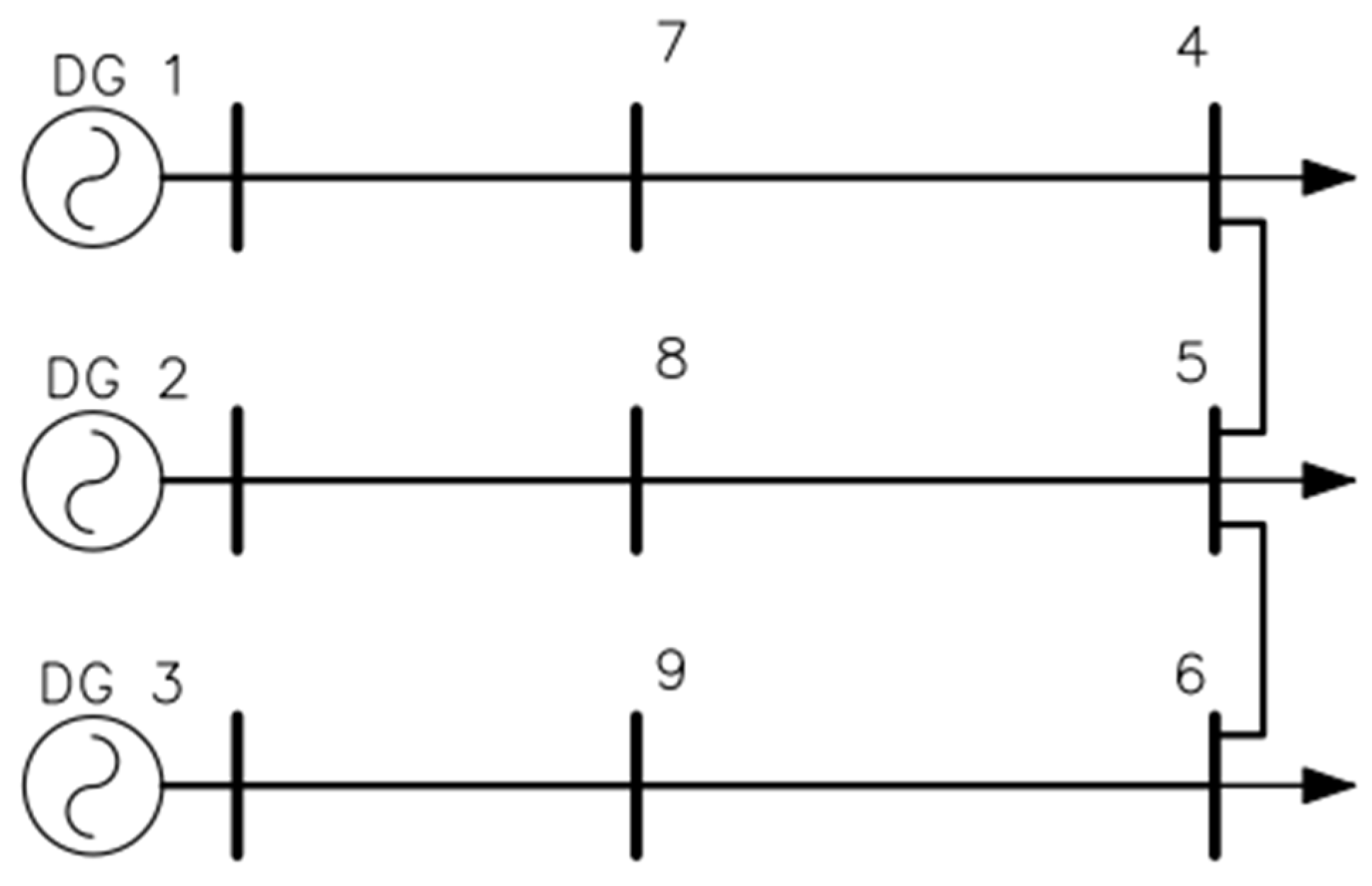
Simulations are carried out with MATLAB software, in a nine bus microgrid (see
Figure 3) having the electrical features reported
Table 1.Three cases with different loading at buses 4–9 are considered to show the efficiency of proposed method.
The optimized solution using the proposed DOPF is compared to a centralized OPF solution using GSO algorithm as described in [
9]. Since the solution of the DOPF is approximated, the attained solution is close to the optimal, but not the optimal. Thus, to get a practical solution, if the network hosts
G generators,
G-1 will implement the DOPF solution, while one will physically act as slack node to account for approximations and small errors in load flow calculations. However, as will be shown using a precise load flow calculation, physically viable results do not differ much from what is attained using the DOPF. From an Initial Operating Point (IOP) of the test system, the DOPF will find new sub-Optimal Operating Point (OOP) for all generators in the test system as well as the voltage at each bus. The precise load flow with one slack bus is then calculated using a conventional Newton Raphson method and the behavior of the optimized system with OOP is checked. In the load flow solution,
G-1 generation units are considered PV buses (in the considered application, these are DG2 and DG3) and the remaining one (typically the largest unit, in the considered application DG1) is the slack bus.
Then the optimal result is compared with the optimal result given by the OPF solution obtained using the GSO method [
9] on the same test system. In the following tables and figures the results are given.
6.1. Case A
Table 2 shows the initial operating point with relevant loading for this operating condition and power losses.
Table 3 shows the sub-optimal solution from the DOPF, OOP.
Table 4 shows the load flow in this latter operating point obtained using DOPF.
Table 5 shows the comparison with the centralized OPF with GSO.
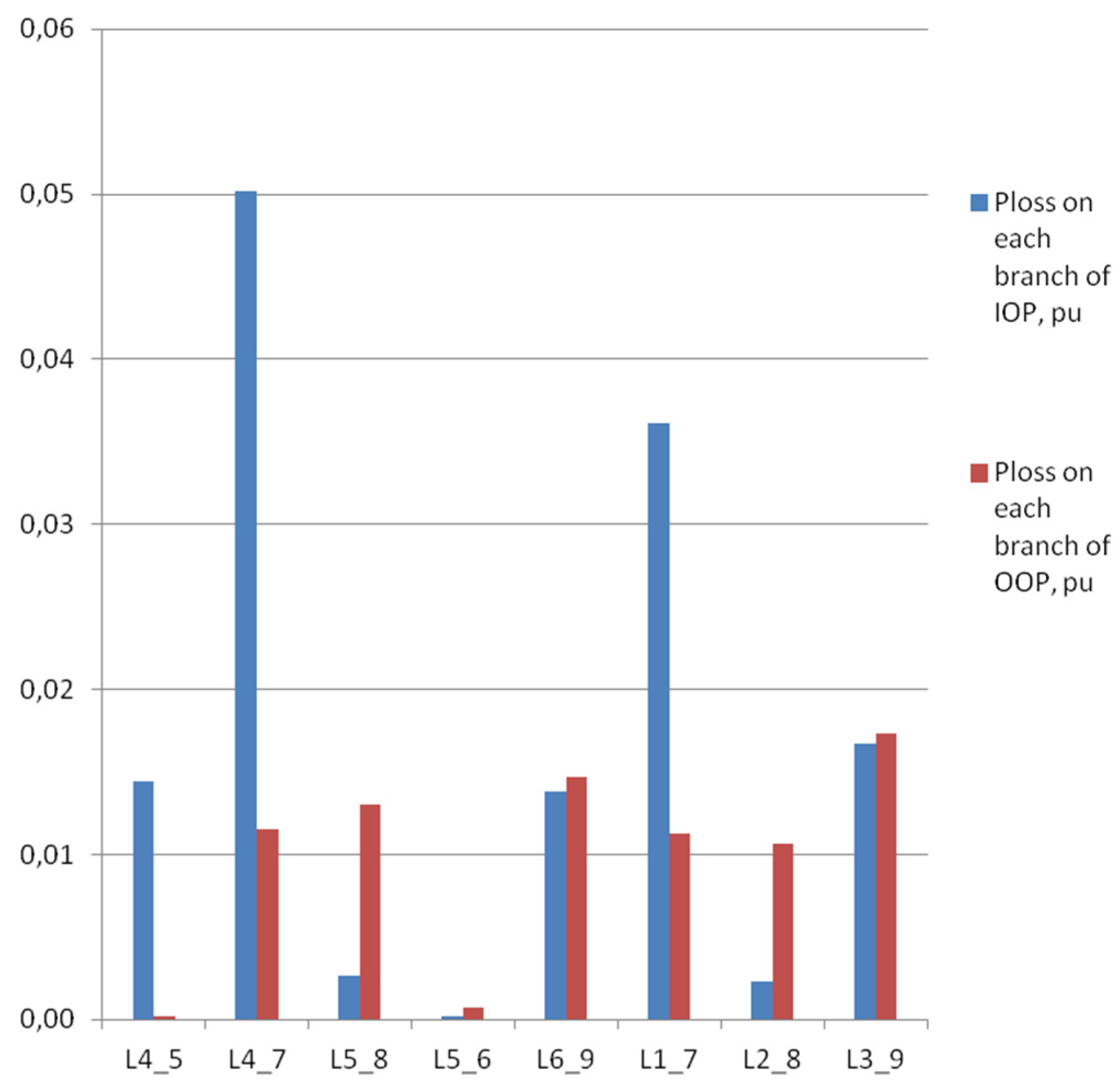
Table 5 shows the error in power losses that is attained considering the two approaches and the latter stays below 4%, while comparing
Table 3 and
Table 4, the maximum voltages estimation error of DOPF is slightly above 4% and with the proposed correction from DOPF power losses are almost half as compared to the IOP.
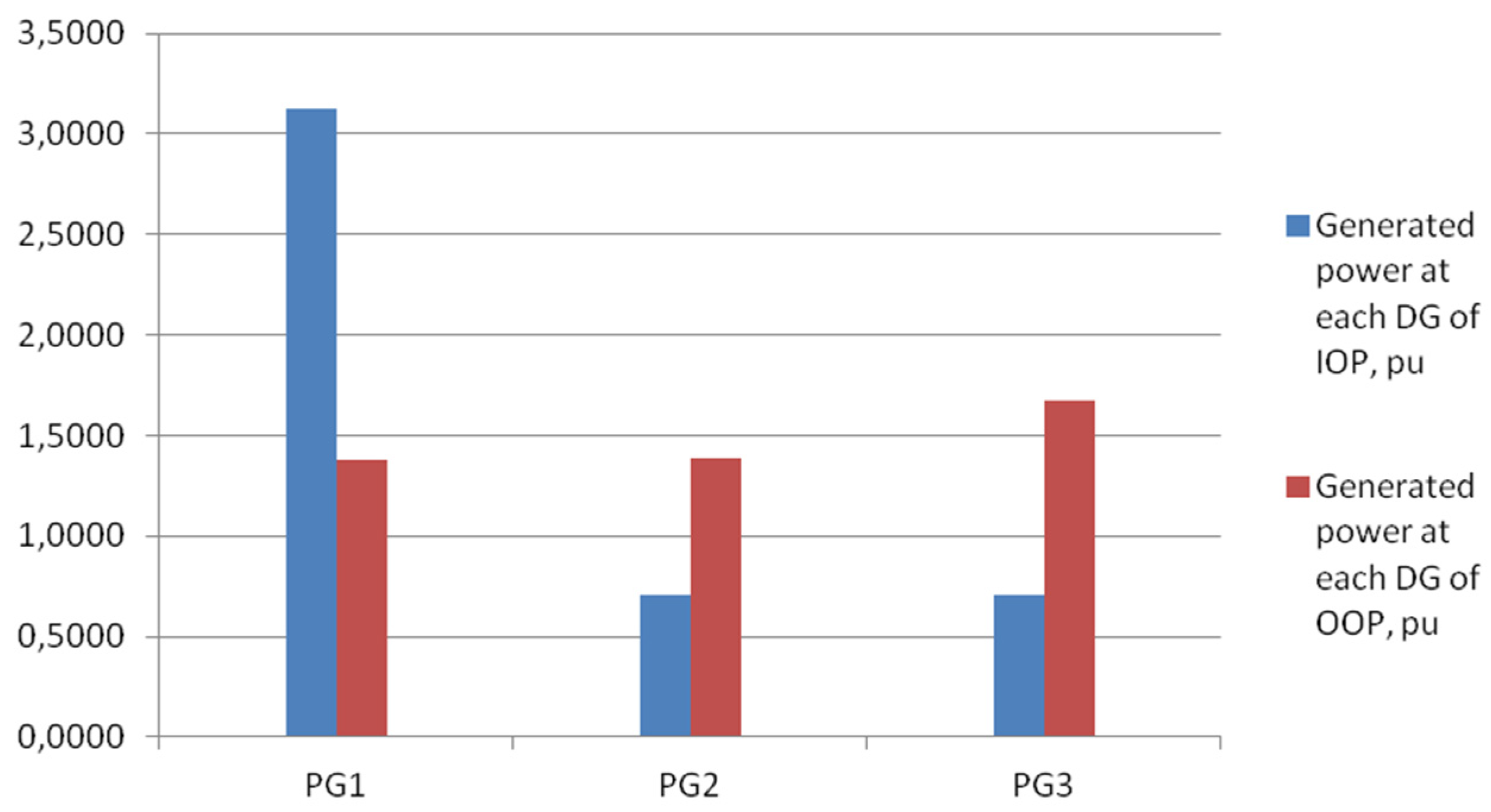
Figure 4 shows the variation of power injection between optimized solution OGPR and initial operating point IOP.
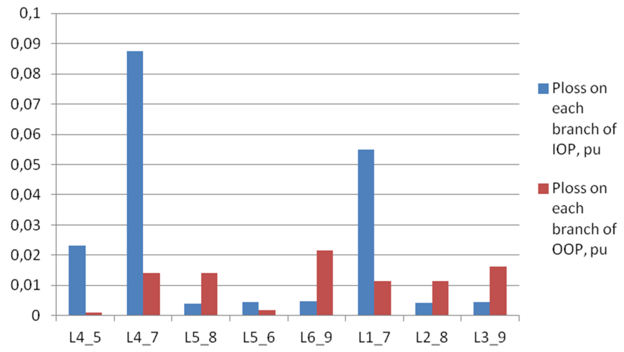
Figure 5 and
Figure 6 show a comparison of the two operating solutions in terms of power losses in branches and voltage level.
Table 2.
Initial operating point.
Table 2.
Initial operating point.
| Bus | Voltage Module Vi/pu | Voltage Angle di/rad | Generated Real Power PGi/pu | Generated Reactive Power QGi/pu | Real power Load PLi/pu | Reactive Power Load QLi/pu | Total Power Losses Ploss/pu |
|---|
| Bus 1 | 1.1090 | 0.0000 | 3.1213 | 0.1334 | 0.0000 | 0.0000 | 0.1874 |
| Bus 2 | 1.1056 | −0.1920 | 0.7097 | 0.4767 | 0.0000 | 0.0000 |
| Bus 3 | 1.1058 | −0.1962 | 0.7064 | 0.5632 | 0.0000 | 0.0000 |
| Bus 4 | 1.0740 | −0.2311 | 0.0000 | 0.0000 | 1.3500 | 0.0000 |
| Bus 5 | 1.0591 | −0.2378 | 0.0000 | 0.0000 | 1.2000 | 0.0000 |
| Bus 6 | 1.0525 | −0.2405 | 0.0000 | 0.0000 | 1.0500 | 0.2132 |
| Bus 7 | 1.1063 | −0.2225 | 0.0000 | 0.0000 | 0.2500 | 0.0508 |
| Bus 8 | 1.0649 | −0.2417 | 0.0000 | 0.0000 | 0.2500 | 0.0508 |
| Bus 9 | 1.0583 | −0.2454 | 0.0000 | 0.0000 | 0.2500 | 0.0508 |
Table 3.
Optimal Operating Point (OOP) given by the DOPF (Distributed Optimal Power Flow).
Table 3.
Optimal Operating Point (OOP) given by the DOPF (Distributed Optimal Power Flow).
| Bus | Vi/pu | PGi/pu |
|---|
| Bus 1 | 1.1090 | 1.4747 |
| Bus 2 | 1.1056 | 1.3884 |
| Bus 3 | 1.1058 | 1.6743 |
| Bus 4 | 1.0714 | |
| Bus 5 | 1.0259 | |
| Bus 6 | 1.0273 | |
| Bus 7 | 1.0890 | |
| Bus 8 | 1.0573 | |
| Bus 9 | 1.0422 | |
Table 4.
Load flow solution of the test system with OOP.
Table 4.
Load flow solution of the test system with OOP.
| Bus | Voltage Module Vi/pu | Voltage Angle di/rad | Generated Real Power PGi/pu | Generated Reactive Power QGi/pu | Real Power Load PLi/pu | Reactive Power Load QLi/pu | Total Power Losses Ploss/Pu |
|---|
| Bus 1 | 1.1090 | 0.0000 | 1.3790 | 0.3628 | 0.0000 | 0.0000 | 0.0917 |
| Bus 2 | 1.1056 | 0.0039 | 1.3884 | 0.2850 | 0.0000 | 0.0000 |
| Bus 3 | 1.1058 | 0.0289 | 1.6743 | 0.2106 | 0.0000 | 0.0000 |
| Bus 4 | 1.0636 | −0.0975 | 0.0000 | 0.0000 | 1.3500 | 0.0000 |
| Bus 5 | 1.0663 | −0.0957 | 0.0000 | 0.0000 | 1.2000 | 0.0000 |
| Bus 6 | 1.0699 | −0.0929 | 0.0000 | 0.0000 | 1.0500 | 0.2132 |
| Bus 7 | 1.0771 | −0.0985 | 0.0000 | 0.0000 | 0.2500 | 0.0508 |
| Bus 8 | 1.0798 | −0.0958 | 0.0000 | 0.0000 | 0.2500 | 0.0508 |
| Bus 9 | 1.0866 | −0.0914 | 0.0000 | 0.0000 | 0.2500 | 0.0508 |
Table 5.
Comparison of results between Glow-worm Swarm Optimization (GSO) and DOPF.
Table 5.
Comparison of results between Glow-worm Swarm Optimization (GSO) and DOPF.
| Method | Ploss/pu | Deviation |
|---|
| DOPF | 0.0917 | 3.97% |
| GSO | 0.0882 |
Figure 4.
Change of generated power at each DG from IOP to OOP.
Figure 4.
Change of generated power at each DG from IOP to OOP.
Figure 5.
Power losses in each branch before (IOP) and after (OOP) the optimization.
Figure 5.
Power losses in each branch before (IOP) and after (OOP) the optimization.
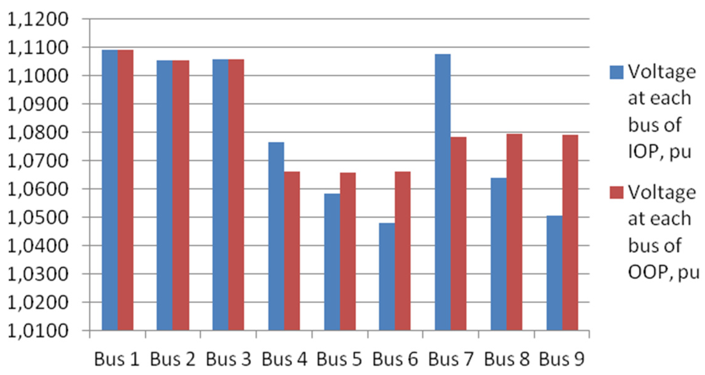
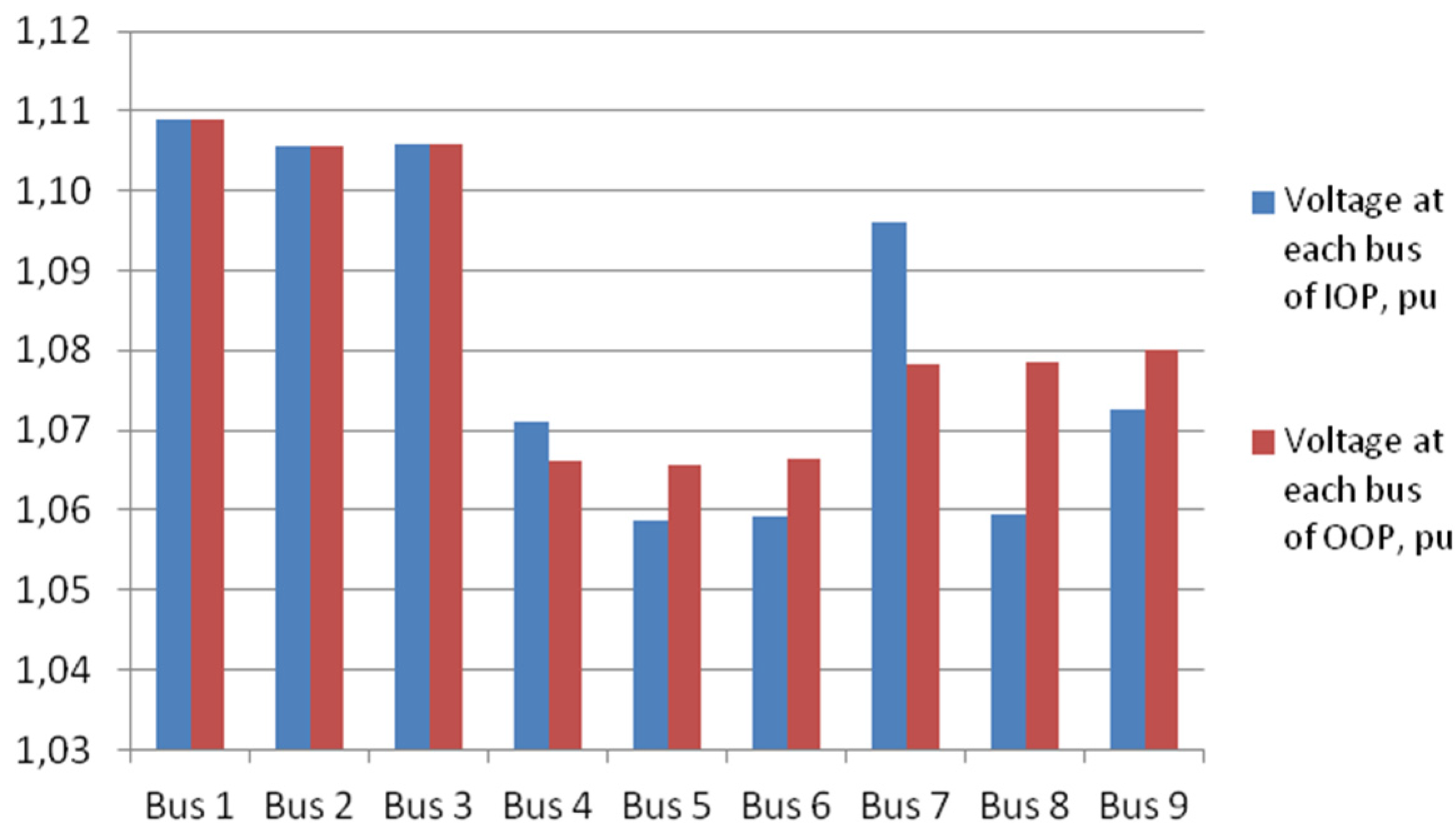
Figure 6.
Voltage improvement at each bus.
Figure 6.
Voltage improvement at each bus.
6.2. Case B
Table 6 shows the initial operating point with relevant power losses.
Table 7 shows the sub-optimal solution from the DOPF, OOP.
Table 8 shows the Load flow in the optimized solution using DOPF.
Table 9 shows a comparison of the solution attained with DOPF and with the centralized OPF with GSO.
Table 9 shows the error in power losses that is attained considering the two approaches and the latter is 1.28%, while comparing
Table 7 and
Table 8, the maximum voltages estimation error of DOPF is slightly above 5% and with the proposed correction from DOPF power losses are almost half as compared to the IOP.
Table 6.
Initial operating point.
Table 6.
Initial operating point.
| Bus | Voltage Module Vi/pu | Voltage Angle di/rad | Generated Real Power PGi/pu | Generated Reactive Power QGi/pu | Real Power Load PLi/pu | Reactive Power Load QLi/pu | Total Power Losses Ploss/pu |
|---|
| Bus 1 | 1.1090 | 0.0000 | 2.5237 | 0.1918 | 0.0000 | 0.0000 | 0.1364 |
| Bus 2 | 1.1056 | −0.1770 | 0.2884 | 0.5635 | 0.0000 | 0.0000 |
| Bus 3 | 1.1058 | −0.0670 | 1.6743 | 0.3882 | 0.0000 | 0.0000 |
| Bus 4 | 1.0712 | −0.1858 | 0.0000 | 0.0000 | 0.9500 | 0.0000 |
| Bus 5 | 1.0588 | −0.1896 | 0.0000 | 0.0000 | 1.2000 | 0.0000 |
| Bus 6 | 1.0592 | −0.1880 | 0.0000 | 0.0000 | 1.0500 | 0.2132 |
| Bus 7 | 1.0960 | −0.1806 | 0.0000 | 0.0000 | 0.3500 | 0.0711 |
| Bus 8 | 1.0596 | −0.1951 | 0.0000 | 0.0000 | 0.2500 | 0.0508 |
| Bus 9 | 1.0726 | −0.1879 | 0.0000 | 0.0000 | 0.5500 | 0.1117 |
Table 7.
OOP given by proposed method.
Table 7.
OOP given by proposed method.
| Bus | Vi/pu | PGi/pu |
|---|
| Bus 1 | 1.1090 | 1.4278 |
| Bus 2 | 1.1056 | 1.3380 |
| Bus 3 | 1.1058 | 1.7205 |
| Bus 4 | 1.0674 | |
| Bus 5 | 1.0036 | |
| Bus 6 | 1.0419 | |
| Bus 7 | 1.0845 | |
| Bus 8 | 1.0501 | |
| Bus 9 | 1.0628 | |
Table 8.
The behavior of the test system with OOP.
Table 8.
The behavior of the test system with OOP.
| Bus | Voltage Module Vi/pu | Voltage Angle di/rad | Generated Real Power PGi/pu | Generated Reactive Power QGi/pu | Real Power Load PLi/pu | Reactive Power Load QLi/pu | Total Power Losses Ploss/pu |
|---|
| Bus 1 | 1.1090 | 0.0000 | 1.3708 | 0.3476 | 0.0000 | 0.0000 | 0.0793 |
| Bus 2 | 1.1056 | −0.0002 | 1.3380 | 0.3004 | 0.0000 | 0.0000 |
| Bus 3 | 1.1058 | 0.0320 | 1.7205 | 0.2935 | 0.0000 | 0.0000 |
| Bus 4 | 1.0662 | −0.0971 | 0.0000 | 0.0000 | 0.9500 | 0.0000 |
| Bus 5 | 1.0656 | −0.0958 | 0.0000 | 0.0000 | 1.2000 | 0.0000 |
| Bus 6 | 1.0665 | −0.0932 | 0.0000 | 0.0000 | 1.0500 | 0.2132 |
| Bus 7 | 1.0783 | −0.0979 | 0.0000 | 0.0000 | 0.3500 | 0.0711 |
| Bus 8 | 1.0785 | −0.0963 | 0.0000 | 0.0000 | 0.2500 | 0.0508 |
| Bus 9 | 1.0802 | −0.0919 | 0.0000 | 0.0000 | 0.5500 | 0.1117 |
Table 9.
Comparison of results between two methods.
Table 9.
Comparison of results between two methods.
| Method | Ploss/pu | % deviation |
|---|
| DOPF | 0.0793 | 1.28% |
| GSO | 0.0783 |
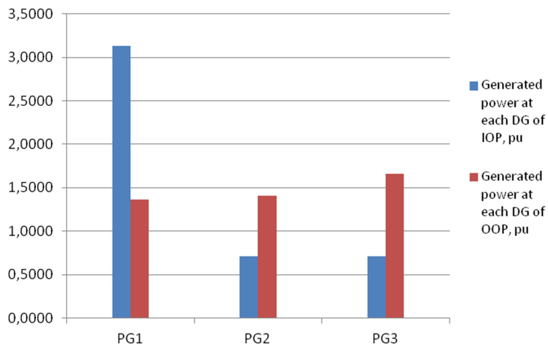
Figure 7 shows the variation of power injection between optimized solution by DOPF, OOP, and initial operating point IOP.
Figure 8 and
Figure 9 show a comparison of the two operating solutions in terms of power losses in branches and bus voltage levels.
Figure 7.
Generated power change at each DG unit.
Figure 7.
Generated power change at each DG unit.
Figure 8.
Power losses in each branch before (IOP) and after (OOP) the optimization.
Figure 8.
Power losses in each branch before (IOP) and after (OOP) the optimization.
Figure 9.
Voltage improvement at each bus.
Figure 9.
Voltage improvement at each bus.
6.3. Case C
Table 10 shows the initial operating point with relevant power losses.
Table 11 shows the sub-optimal solution from the DOPF, OOP.
Table 12 shows the Load flow in the optimized solution using DOPF.
Table 13 shows a comparison of the solution attained with DOPF and with the centralized OPF with GSO.
Table 13 shows the error in power losses that is attained considering the two approaches and the latter is 0.5%, while comparing
Table 11 and
Table 12, the maximum voltages estimation error of DOPF is slightly below 5% and with the proposed correction from DOPF power losses are less than half as compared to the IOP. Losses reduction and voltage profile adjustment show similar behavior as in cases A and B shown in
Section 6.1 and
Section 6.2.
Table 10.
Initial operating point.
Table 10.
Initial operating point.
| Bus | Voltage Module Vi/pu | Voltage Angle di/rad | Generated Real Power PGi/pu | Generated Reactive Power QGi/pu | Real Power Load PLi/pu | Reactive Power Load QLi/pu | Total Power Losses Ploss/pu |
|---|
| Bus 1 | 1.1090 | 0.0000 | 3.1310 | 0.1173 | 0.0000 | 0.0000 | 0.1970 |
| Bus 2 | 1.1056 | −0.1935 | 0.7097 | 0.4877 | 0.0000 | 0.0000 |
| Bus 3 | 1.1058 | −0.1988 | 0.7064 | 0.6629 | 0.0000 | 0.0000 |
| Bus 4 | 1.0765 | −0.2319 | 0.0000 | 0.0000 | 0.9500 | 0.0000 |
| Bus 5 | 1.0583 | −0.2391 | 0.0000 | 0.0000 | 1.2000 | 0.0000 |
| Bus 6 | 1.0482 | −0.2422 | 0.0000 | 0.0000 | 1.0500 | 0.2132 |
| Bus 7 | 1.1077 | −0.2230 | 0.0000 | 0.0000 | 0.3500 | 0.0711 |
| Bus 8 | 1.0641 | −0.2432 | 0.0000 | 0.0000 | 0.2500 | 0.0508 |
| Bus 9 | 1.0505 | −0.2478 | 0.0000 | 0.0000 | 0.5500 | 0.1117 |
Table 11.
OOP given by proposed method.
Table 11.
OOP given by proposed method.
| Bus | Vi/pu | PGi/pu |
|---|
| Bus 1 | 1.109 | 1.4785 |
| Bus 2 | 1.10561 | 1.4104 |
| Bus 3 | 1.1058 | 1.6581 |
| Bus 4 | 1.072644082 | |
| Bus 5 | 1.039476829 | |
| Bus 6 | 1.014015027 | |
| Bus 7 | 1.090245292 | |
| Bus 8 | 1.056166843 | |
| Bus 9 | 1.039240181 | |
Table 12.
The behavior of the test system with OOP.
Table 12.
The behavior of the test system with OOP.
| Bus | Voltage Module Vi/pu | Voltage Angle di/rad | Generated Real Power PGi/pu | Generated Reactive Power QGi/pu | Real Power Load PLi/pu | Reactive Power Load QLi/pu | Total Power Losses Ploss/pu |
|---|
| Bus 1 | 1.1090 | 0.0000 | 1.3603 | 0.3467 | 0.0000 | 0.0000 | 0.0788 |
| Bus 2 | 1.1056 | 0.0062 | 1.4104 | 0.2876 | 0.0000 | 0.0000 |
| Bus 3 | 1.1058 | 0.0277 | 1.6581 | 0.3042 | 0.0000 | 0.0000 |
| Bus 4 | 1.0663 | −0.0963 | 0.0000 | 0.0000 | 0.9500 | 0.0000 |
| Bus 5 | 1.0659 | −0.0950 | 0.0000 | 0.0000 | 1.2000 | 0.0000 |
| Bus 6 | 1.0661 | −0.0926 | 0.0000 | 0.0000 | 1.0500 | 0.2132 |
| Bus 7 | 1.0784 | −0.0971 | 0.0000 | 0.0000 | 0.3500 | 0.0711 |
| Bus 8 | 1.0797 | −0.0951 | 0.0000 | 0.0000 | 0.2500 | 0.0508 |
| Bus 9 | 1.0792 | −0.0917 | 0.0000 | 0.0000 | 0.5500 | 0.1117 |
Table 13.
Comparison of results between two methods.
Table 13.
Comparison of results between two methods.
| Method | Ploss/pu | % deviation |
|---|
| DOPF | 0.0788 | 0.64% |
| GSO | 0.0783 |
6.4. Convergence
The analysis of the convergence is carried out here. Convergence is considered to be reached when the power losses improvement is limited below 1% in two subsequent iterations. Moreover, if power losses do not improve much, operating conditions stay unchanged.
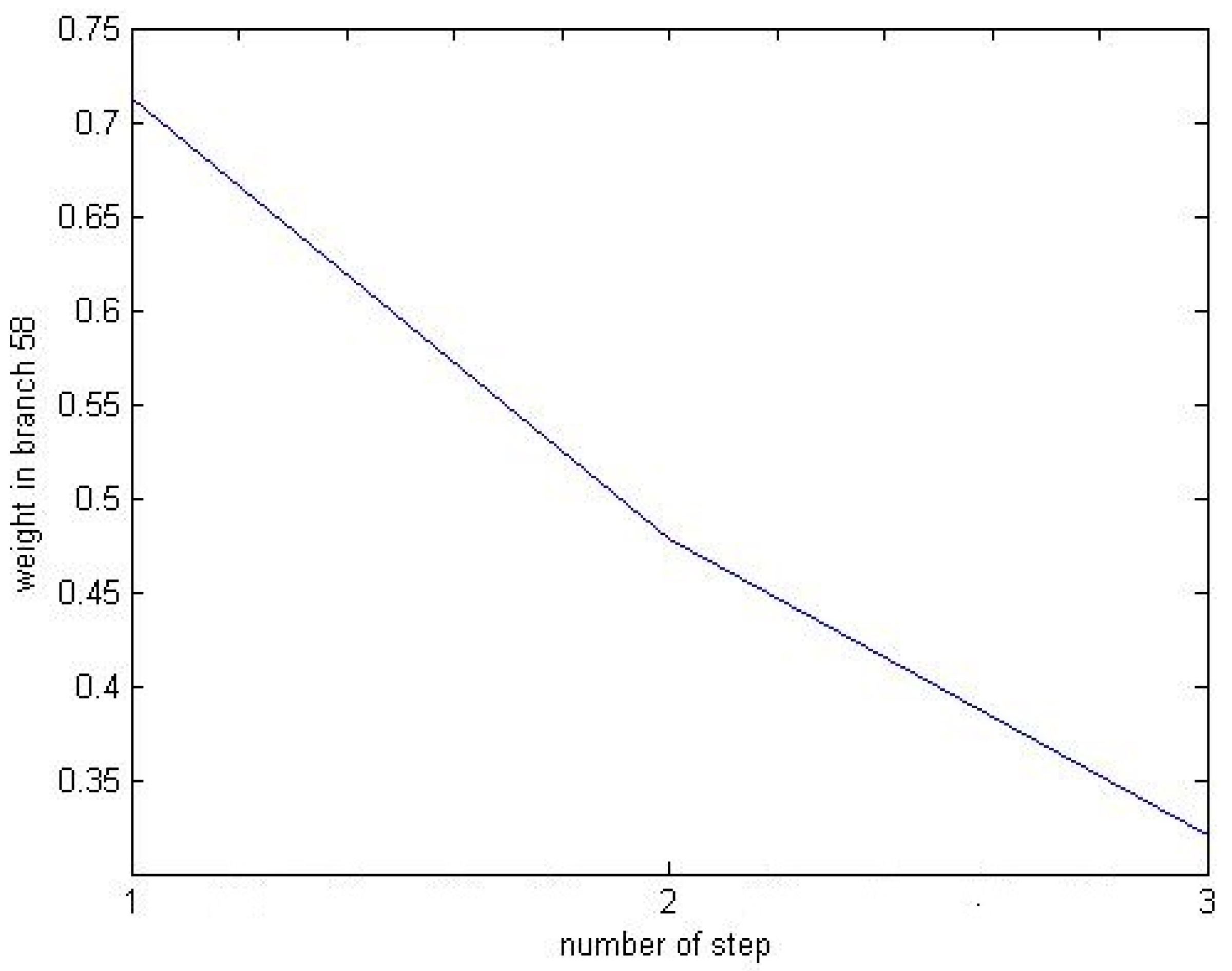
In all experiments, convergence is reached in no more than four iterations. In
Figure 10 it is shown, as an example, how the weight changes in branch
L5_8 during the iterations, going from an initial value of 0.7135 to a final value of 0.3206 after three iterations. Consequently, the initial choice of decreasing power generation of G
2 is changed to growing power generation in this branch, allowing the algorithm to reach results near to the optimum obtained through a centralized algorithm.
Figure 10.
Weights update.
Figure 10.
Weights update.
In future work, the same distributed algorithm will be applied to larger grids and the correction of the injected reactive powers at the generators will be considered.


 and
and 


