Analysis and Optimization Design of a Solar Water Heating System Based on Life Cycle Cost Using a Genetic Algorithm

Abstract

This paper presents an optimization method to design a solar water heating (SWH) system based on life cycle cost (LCC). A genetic algorithm is employed to optimize its configuration and sizing as the optimization technique. To ensure that the optimal solution obtained from the proposed method is a practical design, three constraint conditions, including the energy balance, solar fraction, and available space to install solar collectors, have been set. In addition, the real devices available in the marketplace are considered in the optimization process that searches for optimal configuration and sizing, which is represented by the type and number of each component. By using the proposed method, a SWH system in an office building, South Korea has been designed and optimized. It is observed that a low solar fraction does not always present a decrease in the LCC. A trade-off between the equipment cost and the energy cost results in an optimal design of the SWH system that yields the minimum LCC.

1. Introduction

Global energy consumption has increased steadily over the last few decades and has recently been marked by especially dramatic growth rates in many developing countries, such as China, India, and Brazil. Especially, heating accounts for 40% to 50% of the world’s energy demand and most of the energy supply for heating currently comes from fossil fuels [1]. To reduce the consumption of fossil fuels for heating and the emission of greenhouse gases, solar energy has been accepted as one of the most promising alternative energy sources because it is free and environmentally clean [2]. One of the most widely-known solar thermal applications is the solar water heating (SWH) system [3]. According to the Renewable Energy Policy Network (2010), approximately 70 million houses use SWH systems worldwide [4]. Namely, SWH systems have been recognized as one of the most cost-effective systems to many engineers, investors, and users.

The proper design of SWH systems is important to assure good performance and maximize the economic benefits of these systems. There are many studies in the literature that address the design method of these systems. These design methods can be broadly classified into two categories, namely, correlation-based methods and simulation-based methods [5]. The typical correlation based methods include the $\mathrm{\varphi }$ method [6], $\overline{\mathrm{\varphi }}$ method [7], f-chart method [8], and $\overline{\mathrm{\varphi }},f$-chart method [9]. These design methods have been widely used in preliminary design due to their convenience and inexpensiveness in predicting long-term performance compared to detailed simulation-based methods. The application of these design methods, however, is limited, particularly when the meteorological data and the usage characteristics of the SWH system are different from the data used for corrections [10]. On the other hand, a number of simulation-based methods such as TRNSYS [11] and SOLCHIPS [12] have been applied for the design of SWH systems and are also available on the market as user-friendly software tools. Researchers and designers can numerically evaluate the effects of design variables on long-term energy performance by conducting a series of simulations. These design variables could include the collector area, number of the collectors, storage tank volume, auxiliary heater capacity, and number of the auxiliary heaters. However, even one of these design variables could cause a variation in the SWH system’s performance. Therefore, the number of simulations increases exponentially according to the increase in the number of design variables and parameters. Moreover, these methods also require the involvement of experts and significant computation time.

To overcome these issues in the previously stated correlation and simulation based methods, linear and nonlinear optimization techniques and evolutionary search algorithms have also been applied for the design of SWH systems. Matrawy et al. [13] proposed a graphical method to estimate the optimum collector area and storage volume under a given solar fraction by maximizing the annual system efficiency. Loomans et al. [14] presented a method that designs the sizing of the SWH system with the minimum payback time by a genetic algorithm (GA). Krause et al. [15] optimize the design parameters that are expected to improve the performance of large solar thermal systems. With this optimization, their results show that solar heat cost could be reduced by approximately 18% compared with the conventionally planned system. Kalogirou [16] studied a design method to find the optimum combination of the collector area and storage tank volume to maximize the life cycle savings of a solar installation by using combined artificial neural networks (ANN) with GA. Kulkarni et al. [5] introduced a concept of design space to identify feasible designs of SWH systems. Then, they [17] designed and optimized an active direct SWH system with different storage volumes and collector areas for a given solar fraction by minimizing the annualized life cycle cost. Kim et al. [18] optimized active-indirect SWH systems by minimizing the capital payback period for different energy demands using a μGA. Atia et al. [19] optimized a forced circulation SWH system for an aquaculture system by minimizing the life cycle cost (LCC) using a GA. Yan et al. [10] presented a simplified method for optimizing the key parameters, such as the collector area and the storage tank volume, of SWH systems based on a life cycle energy analysis. Bornatico et al. [20] presented a methodology for finding the optimal size of the main components for a solar thermal system using particle swarm optimization (PSO). Furthermore, several research works have been performed that address the design and sizing of SWH systems using hybrid optimization techniques, such as combined PSO with Hooke-Jeeves [21] and combined GA with binary search method [22].

As previously stated, studies on the optimal design for SWH systems have been increasing and are helpful in identifying the sizing of the SWH systems. However, the number of optimization methods is rather small compared to a wide spread range of correlation and simulation based design methods developed in the last few decades. Furthermore, most of the optimization methods have designed and determined a proper SWH system by examining the appropriate sizing of each component or value of the operation parameters through parametric studies based on objective functions, such as annual efficiency, solar fraction, life cycle savings, LCC, and payback period. In addition, the majority of the studies optimized SWH systems with a given configuration consisting of one type of device for each component. System performance and economic benefits, however, vary considerably depending on even one of these design variables and the relation among them. There are a number of system devices in the marketplace. Each device represents different technical characteristics, which may lead to variation in the energetic and economic performance of SWH systems. Thus, the optimal designs can be different compared to the original designs.

Therefore, this paper presents an optimization method to design a SWH system based on LCC by considering the real devices available in the marketplace. GA is employed to optimize its configuration and sizing as the optimization technique. In addition, this study has been set three constraint conditions, including energy balance, solar fraction, and available space to install solar collectors to ensure that the optimal solution obtained from the proposed method is a practical design. This paper is organized as follows: Section 2 presents the mathematical analysis of an indirect forced SWH system. Section 3 proposes the optimization method by constructing a decision vector, an objective function, and constraints. Section 4 applies the proposed method to optimize the SWH system for an office building in Incheon, South Korea. Finally, some concluding remarks are provided in Section 5.

2. Mathematical Model of SWH System

A schematic diagram of an indirect forced SWH system with a flat plate solar collector array, a heat exchanger, a storage tank, and an auxiliary heater is shown in Figure 1. Solar energy absorbed by a collector array is transferred to the storage tank through an external heat exchanger. When hot water is demanded, heat stored in the tank is supplied to the load. If the storage tank temperature is below the desired hot water temperature, an auxiliary heater is placed in series with the tank and the load supply line is switched on. At any instant in time, the energy balance of a well-mixed storage tank can be described as [5]:

$$\left({\text{ρ}}_w{C}_{p,w}{V}_s\right)\frac{\text{d}{T}_s}{\text{d}t}=q_{Ts}-q_{Ls}-q_l-q_d$$

(1)

where ρ_w, C_p,w are the density (kg/m³) and the specific heat of water (J/kg·°C); V_s is the volume of a storage tank (m³); q_TS, q_l, q_d, and q_Ls are the solar energy supplied to a storage tank (W), the heat loss of a storage tank (W), the discharged heat to avoid overheating of a storage tank (W), and the solar energy extracted from the storage tank (W), respectively.

Figure 1. Schematic diagram of the SWH system considered in this study.

Figure 1. Schematic diagram of the SWH system considered in this study.

The solar energy supplied to the tank (q_TS) is the energy transferred from the useful heat gain of the collector array (q_u) through a heat exchanger according to the differential temperature control. The solar useful gain of identical collector modules in series is [23]:

$$q_u=A_c{N}_{c,s}{\left[F_R\left(\text{τα}\right)I_T-F_R{U}_L\left(T_{ho}-T_a\right)\right]}^{+}$$

(2)

where A_c is the gross area of a single collector module (m²); N_c,s is the number of identical collectors in series; F_R(τα) and F_RU_L are the intercept and the slope of the efficiency curve of identical collector modules in series; I_T is the solar irradiance on the tilted surface (W/m²); T_ho is the hot stream outlet temperature of the heat exchanger (°C); T_a is the outdoor dry-bulb temperature (°C); and the + sign indicates that the collector fluid circulates between the collector array and the hot side of an external heat exchanger only when solar useful heat gain becomes positive, respectively.

For identical collector modules in series, the intercept and slope of the efficiency curve can be estimated as [23]:

$$F_R\left(\text{τα}\right)=F_{R1}{\left(\text{τα}\right)}_1\left[\frac{1-{\left(1-\frac{A_c{F}_{R1}{\left(\text{τα}\right)}_1}{m_c{C}_{p,c}}\right)}^{N_{c,s}}}{N_{c,s}\frac{A_c{F}_{R1}{\left(\text{τα}\right)}_1}{m_c{C}_{p,c}}}\right]$$

(3)

$$F_R{U}_L=F_{R1}{U}_{L1}\left[\frac{1-{\left(1-\frac{A_c{F}_{R1}{\left(\text{τα}\right)}_1}{m_c{C}_{p,c}}\right)}^{N_{c,s}}}{N_{c,s}\frac{A_c{F}_{R1}{\left(\text{τα}\right)}_1}{m_c{C}_{p,c}}}\right]$$

(4)

where F_R1(τα)₁ and F_R1U_L1 are the intercept and the slope of the efficiency curve of a single collector; m_c is the mass flow rate of the collector fluid (kg/s); and C_p,c is the specific heat of the collector fluid (J/kg·°C).

To calculate q_Ts, hot and cold stream outlet temperatures for the plate heat exchanger must be known. Both outlet temperatures can be determined by the effectiveness-number of heat transfer units (NTU-ε) analysis. The NTU-ε method uses three dimensionless parameters, such as the heat exchanger effectiveness (ε), number of exchanger heat transfer units (NTU), and capacity rate ratio (c_r). For a given counter-flow heat exchanger, the three parameters can generally be expressed as [23]:

$$\text{ε}=\{\begin{array}{cc}\hfill \frac{1-exp\left[-NTU\left(1-c_r\right)\right]}{1-c_{r}exp\left[-NTU\left(1-c_r\right)\right]}& , c_r\ne 1\hfill \\ \hfill \frac{NTU}{NTU+1}& , c_r=1\hfill \end{array}$$

(5)

$$c_r=\frac{C_{hex,min}}{C_{hex,max}}$$

(6)

$$NTU=\frac{U{A}_{hex}}{C_{hex,min}}$$

(7)

where UA_hex is product of the overall heat transfer coefficient and area of a heat exchanger (W/°C); C_hex,min and C_hex,max are the smaller and larger values between the hot fluid capacity rate (C_hex,h) and the cold fluid capacity rate (C_hex,c).

The capacity rates of the fluid on the hot and cold sides of the heat exchanger are given as follows:

$$C_{hex,h}=m_c{N}_{c,p}{C}_{p,c}$$

(8)

$$C_{hex,c}=m_c{N}_{c,p}{C}_{p,w}$$

(9)

where N_c,p is the number of parallel connections in the collector array. Therefore, the heat transfer rate (i.e., solar energy supplied to the tank), hot stream outlet temperature, and cold stream outlet temperature can be determined as:

$$q_{Ts}=\{\begin{array}{c}\epsilon C_{hex,h}\left(T_{hi}-T_{ci}\right), C_{hex,min}=C_{hex,h}\\ \epsilon C_{hex,c}\left(T_{hi}-T_{ci}\right), C_{hex,min}=C_{hex,c}\end{array}$$

(10)

$$T_{ho}=T_{hi}-\frac{q_{Ts}}{C_{hex,h}}$$

(11)

$$T_{co}=T_{ci}+\frac{q_{Ts}}{C_{hex,c}}$$

(12)

where T_hi and T_ho are the hot stream inlet and outlet temperatures of the heat exchanger (°C) and T_ci and T_co are the cold stream inlet and outlet temperatures of the heat exchanger (°C).

To satisfy the desired hot water temperature and flow rate, the storage tank discharge flow rate is mixed with make-up water. By considering the mass and energy balance at the mixing junction the flow rate drawn from the tank is determined as:

$$m_s=\{\begin{array}{cc}\hfill m_l\left(\frac{T_l-T_m}{T_s-T_m}\right)& , T_s>T_l\hfill \\ \hfill m_l& , T_s\le T_l\hfill \end{array}$$

(13)

where m_s is the mass flow rate from the storage tank to the load (kg/s); m_l is the mass flow rate of the desired hot water load (kg/s); T_l is the desired hot water temperature (°C); and T_m is the make-up water temperature (°C).

Therefore, the solar energy supplied from the storage tank to the load (q_LS) can be estimated as:

$$q_{Ls}=m_s{C}_{p,w}\left(T_s-T_m\right)$$

(14)

If the storage tank temperature is less than the desired hot water temperature, water discharged from the tank is heated by an auxiliary heater. Auxiliary heating energy can be calculated as:

$$q_{aux}=\{\begin{array}{cc}\hfill 0& , T_s>T_l\hfill \\ \hfill m_l{C}_{p,w}\left(T_l-T_s\right)& , T_s\le T_l\hfill \end{array}$$

(15)

Meanwhile, the storage tank loss (q_l) to the ambient air can be expressed as:

$$q_l=U_s{A}_s\left(T_s-T_{amb}\right)$$

(16)

where U_s and A_s are the heat loss coefficient (W/m²·°C) and the surface area (m²) of a storage tank and T_amb is the ambient temperature (°C).

In this paper, an optimization method is developed to design a SWH system for low temperature applications (below 100 °C) such as a residential hot water system. So if the storage tank temperature is greater than the maximum allowable temperature (T_s,max), the surplus heat will be discharged to avoid overheating of the storage tank. The discharged flow rate and heat can be calculated as:

$$m_d=\{\begin{array}{cc}\hfill \frac{{\text{ρ}}_w{V}_s\left(T_s-T_{s,max}\right)}{\left(T_s-T_m\right)}& , T_s>T_{s,max}\hfill \\ \hfill 0& , T_s\le T_{s,max}\hfill \end{array}$$

(17)

$$q_d=\{\begin{array}{cc}\hfill m_d{C}_{p,w}\left(T_s-T_{s,max}\right)& , T_s>T_{s,max}\hfill \\ \hfill 0& , T_s\le T_{s,max}\hfill \end{array}$$

(18)

The SWH system parameters from Equation (2) to Equation (16) are evaluated on the basis of the initial storage tank temperature at any time step. The final storage tank temperature at the end of any time step must be known because it will be the initial temperature for the next time step. The final storage tank temperature can be estimated as:

$$T_{s,f}=T_s+\frac{\left(q_{Ts}-q_{Ls}-q_l-q_d\right)3,600}{{\text{ρ}}_w{C}_{p,w}{V}_s}∆t$$

(19)

where T_s,f is the final storage tank temperature at the end of any time step.

In this optimization method, the SWH system is operated to meet the hot water demand using differential temperature control on an hourly basis. Hourly demands and weather conditions are required as input data. In the proposed method, the number of heat exchangers is fixed as one because this is the common configuration of forced circulation SWH systems in South Korea. Furthermore, a counter-flow type heat exchanger with UA_hex of 3000 W/°C is used. For the thermal performance of an auxiliary heater, a simple boiler is modeled with its overall efficiency and part load ratio from the device capacity and the energy required to meet the load.

3. Optimization Method of SWH System

3.1. Decision Variable

The optimization method in this paper is developed to determine the optimal configuration and sizing for a SWH system composed of solar collectors, a storage tank, and auxiliary heaters. Here, the configuration means the combination of the selected types for each component and the sizing is computed using its unit capacity and quantity. The capacity units of a solar collector, a storage tank and an auxiliary heater are the area of a collector module (m²), tank volume (m³), and rated heating rate (kW), respectively. This study fixes the number of storage tanks at one because a single tank is generally used in SWH systems for low temperature applications. Therefore, a SWH system is expressed as a decision vector composed of five integer variables that represent the type and number of each component as shown below:

$$x={\left(T_{coll},N_{coll},T_{tank},T_{aux},N_{aux}\right)}^T$$

(20)

where T_coll is the type of solar collectors; N_coll is the number of solar collectors; T_tank is the type of storage tanks; T_aux is the type of auxiliary heaters; and N_aux is the number of auxiliary heaters.

3.2. Objective Function

This design method obtains the optimal configuration and sizing of a SWH system by minimizing the LCC of the system, which includes all of the costs throughout the lifetime of the system. It can be formulated as follows [24]:

$$C_{LCC}=C_I+C_M+C_R+C_E-C_S$$

(21)

where C_I, C_M, C_R, C_E, and C_S represent the initial, maintenance, replacement, energy, and subsidy costs, respectively.

The initial cost is related to the direct purchase cost of the main components and the supplementary cost, as follows:

$$C_I=\left(C_{coll,j}{N}_{coll}+C_{tank,j}+C_{aux,j}{N}_{aux}\right)\left(1+R_I\right)$$

(22)

where C_coll,j, C_tank,j, and C_aux,j are the purchase price of the $j$th device of solar collectors, storage tanks, and auxiliary heaters; $N_{coll}$ and N_aux are the installation number of the jth device of solar collectors and auxiliary heaters; and R_I is a percentage of the supplementary cost against the direct purchase cost.

The maintenance cost is calculated as a percentage of the initial cost of a SWH system, described as follows:

$$C_M=C_I{R}_M\left[\frac{{\left(1+i\right)}^{n_p}-1}{i{\left(1+i\right)}^{n_p}}\right]$$

(23)

where R_M is a percentage of the annual maintenance cost against the initial cost; n_p is the planning period; and i is the real discount rate.

The replacement costs are incurred depending on each component’s lifetime during the planning period and are described as follows:

$$C_{R,c}={\displaystyle \sum }_{n_{r,c}=1}^{n_{r,c}}\left\{C_{I,c}\left[\frac{1}{{\left(1+i\right)}^{\left(n_{l,c}{n}_{r,c}\right)}}\right]\right\}$$

(24)

where C_R,c and C_I,c are the replacement costs and the initial costs of each component; n_l,c is the lifetime of each component; and n_r,c is the replacement times of each component.

The energy cost is computed by applying the electricity and liquid natural gas (LNG) escalation rate and is described as follows:

$$C_E=UP{A}_{ELE}^{\text{*}}{\displaystyle \sum }_{t=1}^{8,760}{c}_{ELE}\left(t\right)F_{ELE}\left(t\right)+UP{A}_{LNG}^{\text{*}}{\displaystyle \sum }_{t=1}^{8,760}{c}_{LNG}\left(t\right)F_{LNG}\left(t\right)$$

(25)

$$UP{A}_{fuel}^{\text{*}}=\frac{\left(\frac{1+e_{fuel}}{1+i}\right)\left[{\left(\frac{1+e_{fuel}}{1+i}\right)}^{n_p}-1\right]}{\left(\frac{1+e_{fuel}}{1+i}\right)-1}$$

(26)

where $UP{A}_{ELE}^{*}$ and $UP{A}_{LNG}^{*}$ are the uniform present value factor adjusted to reflect the electricity and the LNG price escalation rate, c_ELE and c_LNG are the hourly electricity cost [KRW/kWh] and hourly LNG cost [KRW/m³] for a SWH system; F_ELE and F_LNG are the hourly electricity consumption [kWh] and hourly LNG consumption [m³]; and e_fuel is the fuel price escalation rate.

It is considered that part of the initial cost is backed by the government depending on the related regulations regarding the installation of renewable energy systems. According to the total gross area of the collector modules, the subsidy cost is calculated as follows:

$$C_S=\{\begin{array}{cc}\hfill C_I{R}_S& , A_{R,max}>A_{coll,j}{N}_{coll}\hfill \\ \hfill \left[C_{coll,j}floor\left(\frac{A_{R,max}}{A_{coll,j}}\right)+C_{tank,j}+C_{aux,j}{N}_{aux}\right]\left(1+R_I\right)R_S& , A_{R,max}\le A_{coll,j}{N}_{coll}\hfill \end{array}$$

(27)

where A_coll,j is the gross area of the jth device of solar collectors (m²); A_R,max is the maximum capacity available to receive the subsidy cost (m²); and R_S is a percentage of the subsidy cost against the initial cost (%).

3.3. Constraint Conditions

The constraints restrict each decision variable to take a value within the minimum and the maximum limits. In this paper, the decision variables present the type and number of main components for a SWH system. Most previous studies that optimized a particular SWH system consisting of only one model selected beforehand by researchers had to constraint the limits of each decision variable. However, when optimizing the types of component that has different capacities, it is difficult to set the maximum limits of decision variables that indicate the number of components to the specific values because the limits vary according to the device types. Therefore, this study has set the following inequality constraints, namely the energy balance, the solar fraction, and the available space to install the collectors that are used in the practical design problems of a SWH system. The limits of N_aux are determined by Equation (26) and the limits of N_coll are restricted by Equations (27) and (28). Meanwhile, the limits of the decision variables (T_coll, T_tank, and T_aux) that denote the types of components are set automatically at the number of types in the inputted data tables of each component.

(a)

Energy balance:

$$Q_{L,peak}\le Q_{aux,tot}$$

(28)

(b)

Solar fraction (penetration of the solar energy):

$$F_{S,min}\le F_S\le F_{S,max}$$

(29)

(c)

Available space to install the collector array:

$$A_{c,ins}\le A_{c,max}$$

(30)

with

$$Q_{aux,tot}=Q_{aux,j}{N}_{aux}$$

(31)

$$F_S=\left(1-\frac{Q_{aux,year}}{Q_{L,year}}\right)\times 100$$

(32)

$$A_{c,ins}=N_{coll}{W}_{coll,j}{H}_{coll,j}\left[cos\left({\text{β}}_{coll}\right)+\frac{sin\left({\text{β}}_{coll}\right)}{tan\left({\text{α}}_{s,w}\right)}\right]$$

(33)

where Q_L,peak is the peak load (kW); Q_aux,j is the heating capacity of the $j$th device of auxiliary heaters (kW); Q_L,year is the annual hot water load (kWh); Q_aux,tot is the total heating capacity of the auxiliary heaters (kW); F_S,min and F_S,max are the minimum and the maximum solar fractions (%); F_S is the solar fraction of any SWH system; W_coll,j and H_coll,j are the width and the height of the j th module of solar collectors (m); β_coll is the slope of the collector array (°); α_s,w is the meridian altitude in winter (°); A_c,max is the available space to install solar collectors (m²); and A_c,ins is the installation area of the solar collectors (m²).

3.4. Optimization Algorithm

This study uses the real coded GA [25] to optimize the configuration and sizing for a SWH system. The GA parameters used for the implementation of the optimization algorithm are: number of generations = 300, population size = 50, crossover probability = 0.9, and mutation probability = 0.7. In this paper the optimization process using a GA terminated when the maximum number of generations has been reached. The modified crossover and mutation suggested by Ko et al. [26] was also applied to treat the decision variables that represent the type and number of components as a discrete.

Meanwhile, as described in Section 3.1, a decision vector composed of five integer variables that represent the type and number of each component. In the GA process, the types of a decision vector are recognized as the identification numbers assigned in the inputted data tables of each component. Thus, the identification numbers and installation numbers of each component act as genes during the evolutionary process. In addition, the technical and economic data of the devices corresponding to the identification numbers of each component are used as input data in the energetic and economic estimation of the SWH systems.

4. Simulation Results and Discussion

4.1. Simulation Parameters or Data

The proposed optimization method was applied for the design and optimal configuration sizing of a SWH system for an office building in Incheon at Latitude 36° N and Longitude 125° E, South Korea.

In the present study, three different hot water consumptions of weekday, Saturday and Sunday are distributed during a day according to the hot water load profile of the typical office building [27] as shown in Figure 2. Daily hot water consumptions of weekday, Saturday and Sunday are 4.00, 1.91 and 0.84 m³/day at 60 °C, respectively. The meteorological conditions during the year are illustrated in Figure 3. The average daily solar irradiance is 3.38 kW/m², and the average hourly air temperature is 12.18 °C, respectively.

Figure 2. Hourly hot water consumptions over one day in a case study building.

Figure 2. Hourly hot water consumptions over one day in a case study building.

Figure 3. (a) Hourly global horizontal solar irradiance, and (b) outdoor air temperature and make-up water temperature over one year for Incheon, South Korea.

Figure 3. (a) Hourly global horizontal solar irradiance, and (b) outdoor air temperature and make-up water temperature over one year for Incheon, South Korea.

The SWH system of the case study is comprised of three main components, namely, five types of solar collectors, ten types of storage tanks, and eight types of auxiliary heaters. The technical and economical characteristics of the solar collectors, storage tanks, and auxiliary heaters used in the optimization design are shown in Table 1, Table 2 and Table 3.

All devices shown in Table 1, Table 2 and Table 3 are available in the actual market, and a list of these devices can be extended by the researcher and designer. Moreover, manufactured devices in the actual market do not have constant size increments and represent different technical characteristics. Therefore, it is expected to be able to practically evaluate the energetic and economic performance of SWH systems and obtain more realistic and optimal designs by using the different types of devices for each component.

Table 1. Technical and economic parameters of the solar collectors for the case study.

Parameters	Types
	0	1	2	3	4
Useful gain (kWh/m2 day)	2.228	2.361	2.417	2.444	2.556
Intercept of the collector efficiency (–)	0.7200	0.7208	0.7445	0.7043	0.7203
Negative of the slope of the collector efficiency (W/m2·°C)	4.09	4.7999	4.8483	4.5368	3.9488
Flow rate of the fluid at standard condition (kg/s)	0.0400	0.0373	0.0381	0.0368	0.0533
Overall height (m)	2.00	2.00	2.00	2.00	2.40
Overall width (m)	1.00	1.00	1.00	0.99	1.18
Lifetime (years)	20	20	20	20	20
Purchase cost (1,000 KRW/ea.)	520	530	545	540	820

Table 1. Technical and economic parameters of the solar collectors for the case study.

Parameters	Types
	0	1	2	3	4
Useful gain (kWh/m2 day)	2.228	2.361	2.417	2.444	2.556
Intercept of the collector efficiency (–)	0.7200	0.7208	0.7445	0.7043	0.7203
Negative of the slope of the collector efficiency (W/m2·°C)	4.09	4.7999	4.8483	4.5368	3.9488
Flow rate of the fluid at standard condition (kg/s)	0.0400	0.0373	0.0381	0.0368	0.0533
Overall height (m)	2.00	2.00	2.00	2.00	2.40
Overall width (m)	1.00	1.00	1.00	0.99	1.18
Lifetime (years)	20	20	20	20	20
Purchase cost (1,000 KRW/ea.)	520	530	545	540	820

Table 2. Technical and economic parameters of the storage tanks for the case study.

Parameters	Types
	0	1	2	3	4	5	6	7	8	9
Tank volume (m3)	0.44	0.96	1.72	2.65	3.76	4.91	5.54	6.21	6.92	9.58
Heat loss coefficient (W/°C)	0.3	0.3	0.3	0.3	0.3	0.3	0.3	0.3	0.3	0.3
Overall height (m)	1.22	1.22	1.52	2.00	2.44	2.44	2.44	2.44	3.05	3.05
Overall diameter (m)	0.68	1.00	1.20	1.30	1.40	1.60	1.70	1.80	1.70	2.00
Lifetime (years)	15	15	15	15	15	15	15	15	15	15
Purchase cost (1,000,000 KRW/ea.)	6.60	7.15	9.49	10.73	12.65	15.88	17.33	18.02	18.98	24.20

Table 2. Technical and economic parameters of the storage tanks for the case study.

Parameters	Types
	0	1	2	3	4	5	6	7	8	9
Tank volume (m3)	0.44	0.96	1.72	2.65	3.76	4.91	5.54	6.21	6.92	9.58
Heat loss coefficient (W/°C)	0.3	0.3	0.3	0.3	0.3	0.3	0.3	0.3	0.3	0.3
Overall height (m)	1.22	1.22	1.52	2.00	2.44	2.44	2.44	2.44	3.05	3.05
Overall diameter (m)	0.68	1.00	1.20	1.30	1.40	1.60	1.70	1.80	1.70	2.00
Lifetime (years)	15	15	15	15	15	15	15	15	15	15
Purchase cost (1,000,000 KRW/ea.)	6.60	7.15	9.49	10.73	12.65	15.88	17.33	18.02	18.98	24.20

Table 3. Technical and economic parameters of the auxiliary heaters for the case study.

Parameters	Types
	0	1	2	3	4	5	6	7
Rated heating capacity (kW)	15.12	18.61	23.26	29.08	34.89	58.15	81.41	116.30
Rated efficiency (%)	83	84	85	86	86	82	83	83
Lifetime (years)	15	15	15	15	15	15	15	15
Purchase cost (1000 KRW/ea.)	807	844	909	964	1,039	2,291	2,565	3,207

Table 3. Technical and economic parameters of the auxiliary heaters for the case study.

Parameters	Types
	0	1	2	3	4	5	6	7
Rated heating capacity (kW)	15.12	18.61	23.26	29.08	34.89	58.15	81.41	116.30
Rated efficiency (%)	83	84	85	86	86	82	83	83
Lifetime (years)	15	15	15	15	15	15	15	15
Purchase cost (1000 KRW/ea.)	807	844	909	964	1,039	2,291	2,565	3,207

Design parameters and assumptions required for the optimization process are summarized in Table 4. Table 5 shows the electricity and liquid natural gas tariff for an office building. These data are based on the actual conditions in South Korea.

Table 4. Optimization design parameters considered in the case study.

Parameters	Value
Slope of collector array (°)	35
Azimuth of collector array (°)	0
Meridian altitude in winter season (°)	29
Desired hot water temperature (°C)	60
Maximum allowable storage tank temperature (°C)	100
Temperature of the environment surrounding the storage tank (°C)	20
Specific heat of collector fluid (J/kg·°C)	3560
Specific heat of water (J/kg·°C)	4180
Density of collector fluid (kg/m3)	1043
Density of water (kg/m3)	1000
Product of the overall heat transfer coefficient and area of a heat exchanger (W/°C)	3000
Maximum number of collectors in series (ea.)	6
Project lifetime (years)	40
Real discount rate (%)	2.91
Nominal interest rate (%)	6.00
Inflation rate (%)	3.00
Electricity cost escalation rate (%)	4.00
Gas cost escalation rate (%)	4.00
Maximum capacity available to receive the subsidy cost (m2)	500
Area available to install solar collectors (m2)	600
Supplementary cost ratio against the purchase cost (%)	30
Maintenance cost ratio against the initial cost (%)	1.5
Subsidy cost ratio against the initial cost (%)	50

Table 4. Optimization design parameters considered in the case study.

Parameters	Value
Slope of collector array (°)	35
Azimuth of collector array (°)	0
Meridian altitude in winter season (°)	29
Desired hot water temperature (°C)	60
Maximum allowable storage tank temperature (°C)	100
Temperature of the environment surrounding the storage tank (°C)	20
Specific heat of collector fluid (J/kg·°C)	3560
Specific heat of water (J/kg·°C)	4180
Density of collector fluid (kg/m3)	1043
Density of water (kg/m3)	1000
Product of the overall heat transfer coefficient and area of a heat exchanger (W/°C)	3000
Maximum number of collectors in series (ea.)	6
Project lifetime (years)	40
Real discount rate (%)	2.91
Nominal interest rate (%)	6.00
Inflation rate (%)	3.00
Electricity cost escalation rate (%)	4.00
Gas cost escalation rate (%)	4.00
Maximum capacity available to receive the subsidy cost (m2)	500
Area available to install solar collectors (m2)	600
Supplementary cost ratio against the purchase cost (%)	30
Maintenance cost ratio against the initial cost (%)	1.5
Subsidy cost ratio against the initial cost (%)	50

Table 5. Electricity and liquid natural gas tariffs.

Classification			Value
Electricity	Basic charge		6160
	Energy charge (KRW/kWh)	Summer (June, July and August)	105.7
		Spring/Fall (March, April, May, September, and October)	65.2
		Winter (November, December, January and February)	92.3
Natural gas	Energy charge (KRW/MJ)	Summer (May, June, July, August and September)	19.26
		Spring/Fall (April, October and November)	19.28
		Winter (December, January, February and March)	19.46

Table 5. Electricity and liquid natural gas tariffs.

Classification			Value
Electricity	Basic charge		6160
	Energy charge (KRW/kWh)	Summer (June, July and August)	105.7
		Spring/Fall (March, April, May, September, and October)	65.2
		Winter (November, December, January and February)	92.3
Natural gas	Energy charge (KRW/MJ)	Summer (May, June, July, August and September)	19.26
		Spring/Fall (April, October and November)	19.28
		Winter (December, January, February and March)	19.46

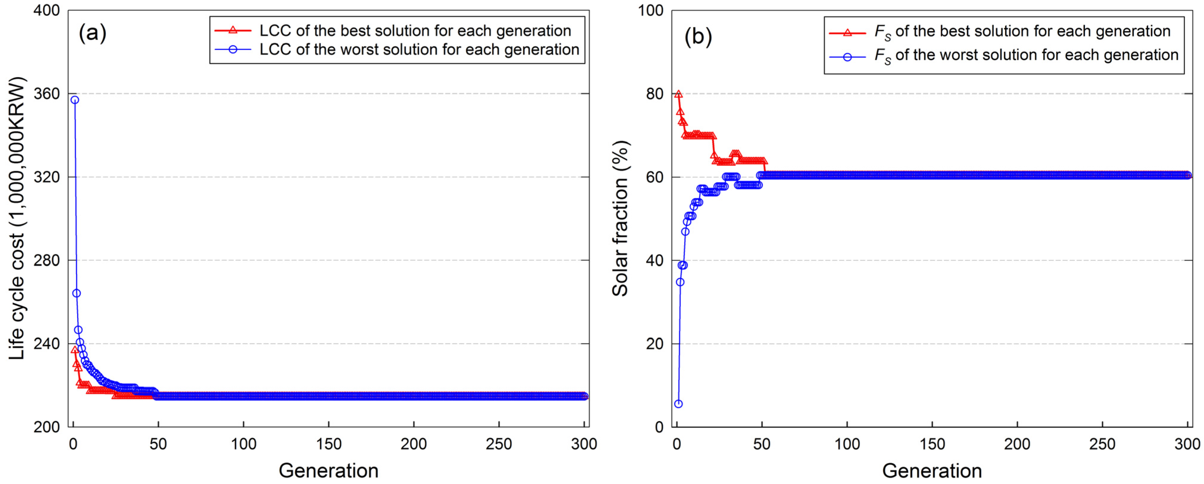
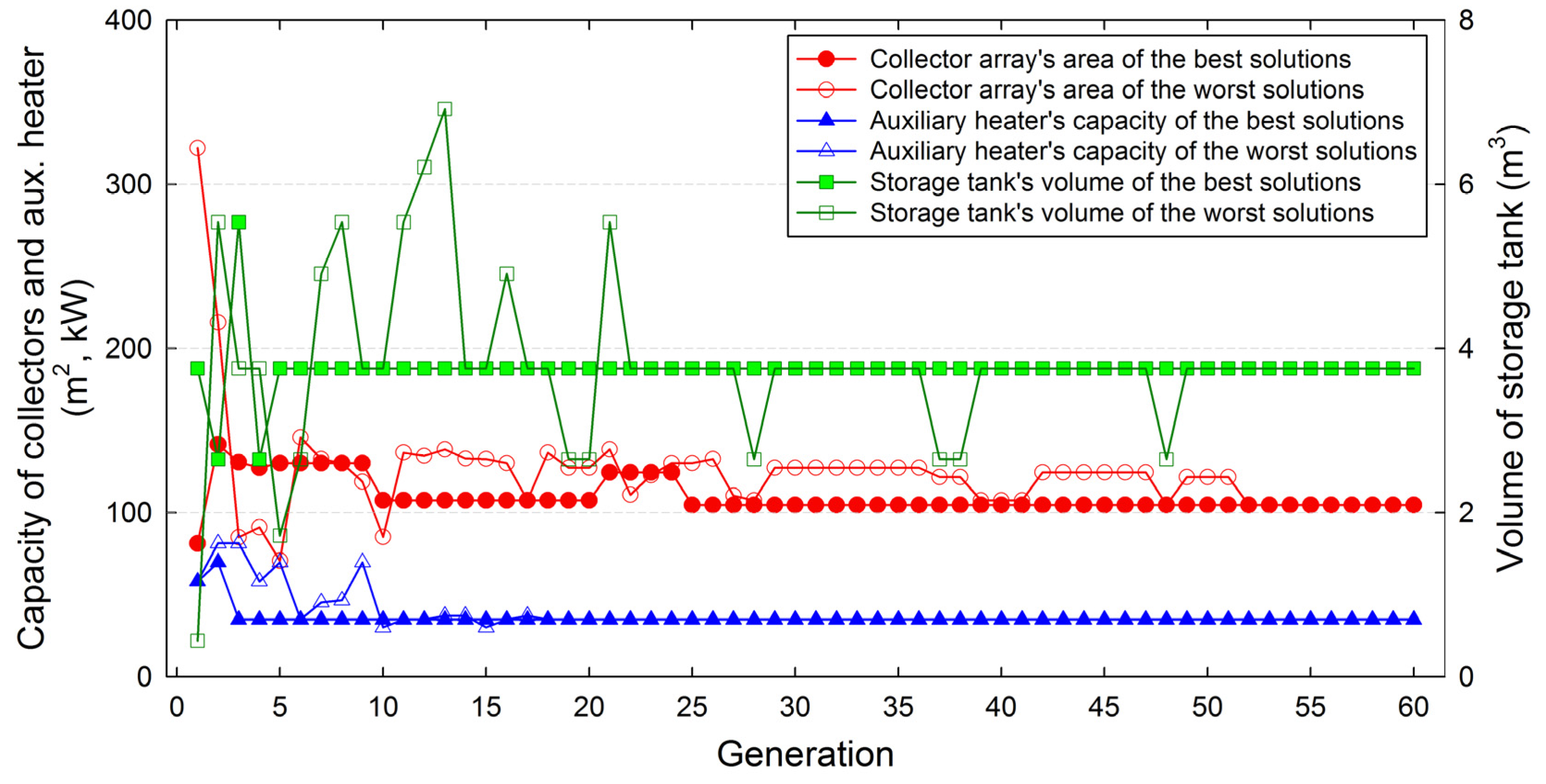
4.2. Optimization Results of the Base Case

A case study was conducted to find the optimal SWH system that represents the minimum LCC without restriction for the solar fraction using the proposed optimization method. The minimum and maximum solar fractions of the base case were set as 0% and 100%, respectively.

Figure 4 shows the evolution of the objective function and the solar fraction for the base case. As indicated in Figure 4a, the minimum LCC of 214.7 million KRW (approximately 194.3 thousand USD) has been derived for the first time in the 25 generations, and the optimization algorithm was finally converged in 52 generations. Therefore, 300 generations can be considered as fair termination conditions. Compared to the values of the objective function for the best and worst solutions in the initial population that was randomly generated, an LCC of 9.31% and 39.86% can be reduced using the proposed optimization method.

Figure 4. Evolution of (a) the objective function and (b) the solar fraction during the optimization process for the base case.

Figure 4. Evolution of (a) the objective function and (b) the solar fraction during the optimization process for the base case.

Meanwhile, the optimization algorithm converges toward a solar fraction of 60.42% in the base case. As indicated in Figure 4b, the solar fractions of the best and worst solutions for each generation were converged to the solar fraction of the optimal solution, while increasing and decreasing, respectively. It is interesting to note that a high solar fraction of a SWH system does not always present an increase in the LCC against what a lot of engineers would think. In other words, to design an economically feasible SWH system by simply adjusting the solar fraction is very difficult, and it is necessary to design the optimal configuration and sizing of the system by using the optimization method.

The variation in component size for the best and worst solutions during 60 generations can be observed in Figure 5. From Figure 4 and Figure 5, it can be seen that the optimization algorithm identifies and assesses various possible SWH systems to significantly improve the objective function at the beginning of the optimization process. In the subsequent generations, the objective function is gradually improved by minutely adjusting the type and number of components that form each combination. Subsequently, the optimization algorithm obtains the optimal configuration and sizing of the SWH system with the minimum LCC. Table 6 shows the optimal SWH system of the base case and its technical and economic characteristics. It can be seen from this table that the optimal SWH system consists of solar collectors of 104.71 m², a storage tank of 3.76 m³, and an auxiliary heater of 34.89 kW.

Meanwhile, using an Intel(R) Core(TM) i5–2310 @2.90GHz_CPU and 4 GB memory computer, the developed method requires approximately three minutes to optimize the SWH system of the case study. This result indicates that the proposed design method can obtain an optimal SWH system within a short computation time.

Figure 5. Variation of component size for the best and worst solutions in each generation for the base case.

Figure 5. Variation of component size for the best and worst solutions in each generation for the base case.

Table 6. Characteristics of the optimal SWH system for the base case.

Variable	Description	Value
$T_{coll}$	Type of the solar collector (–)	4
$N_{coll}$	Number of the solar collectors (ea.)	37
$T_{tank}$	Type of the storage tank (–)	4
$T_{aux}$	Type of the auxiliary heater (–)	4
$N_{aux}$	Number of the auxiliary heaters (ea.)	1
$A_{c,tot}$	Total area of the solar collector (m2)	104.71
$V_s$	Volume of the storage tank (m3)	3.76
$Q_{aux,tot}$	Capacity of the auxiliary heaters (kW)	34.89
$A_{c,ins}$	Installation area of the solar collectors (m2)	194.3
$Q_{L,peak}$	Peak hot water load (kW)	27.35
$Q_{L,year}$	Annual hot water load (kWh/year)	60,218
$I_T$	Annual solar irradiance on the collector array (kWh/year)	137,495
$Q_u$	Annual useful heat gain of the collector array (kWh/year)	39,986
$Q_{Ts}$	Annual solar energy supplied to the storage tank (kWh/year)	37,332
$Q_l$	Annual heat loss of the storage tank (kWh/year)	752
$Q_d$	Annual discharged heat from the storage tank (kWh/year)	4
$Q_{Ls}$	Annual solar energy supplied by the storage tank (kWh/year)	36,386
$Q_{aux}$	Annual auxiliary energy supplied by the heaters (kWh/year)	23,832
$F_{LNG}$	Annual LNG consumption (m3/year)	2562
$F_{ELE}$	Annual electricity consumption (kWh/year)	1413
$F_S$	Annual solar fraction (%)	60.42
$C_I$	Initial cost (1000 KRW)	57,238
$C_M$	Maintenance cost (1000 KRW)	20,129
$C_R$	Replacement cost (1000 KRW)	41,302
$C_E$	Energy cost (1000 KRW)	124,616
$C_S$	Subsidy cost (1000 KRW)	28,619
$C_{LCC}$	Life cycle cost (1000 KRW)	214,666

Table 6. Characteristics of the optimal SWH system for the base case.

Variable	Description	Value
$T_{coll}$	Type of the solar collector (–)	4
$N_{coll}$	Number of the solar collectors (ea.)	37
$T_{tank}$	Type of the storage tank (–)	4
$T_{aux}$	Type of the auxiliary heater (–)	4
$N_{aux}$	Number of the auxiliary heaters (ea.)	1
$A_{c,tot}$	Total area of the solar collector (m2)	104.71
$V_s$	Volume of the storage tank (m3)	3.76
$Q_{aux,tot}$	Capacity of the auxiliary heaters (kW)	34.89
$A_{c,ins}$	Installation area of the solar collectors (m2)	194.3
$Q_{L,peak}$	Peak hot water load (kW)	27.35
$Q_{L,year}$	Annual hot water load (kWh/year)	60,218
$I_T$	Annual solar irradiance on the collector array (kWh/year)	137,495
$Q_u$	Annual useful heat gain of the collector array (kWh/year)	39,986
$Q_{Ts}$	Annual solar energy supplied to the storage tank (kWh/year)	37,332
$Q_l$	Annual heat loss of the storage tank (kWh/year)	752
$Q_d$	Annual discharged heat from the storage tank (kWh/year)	4
$Q_{Ls}$	Annual solar energy supplied by the storage tank (kWh/year)	36,386
$Q_{aux}$	Annual auxiliary energy supplied by the heaters (kWh/year)	23,832
$F_{LNG}$	Annual LNG consumption (m3/year)	2562
$F_{ELE}$	Annual electricity consumption (kWh/year)	1413
$F_S$	Annual solar fraction (%)	60.42
$C_I$	Initial cost (1000 KRW)	57,238
$C_M$	Maintenance cost (1000 KRW)	20,129
$C_R$	Replacement cost (1000 KRW)	41,302
$C_E$	Energy cost (1000 KRW)	124,616
$C_S$	Subsidy cost (1000 KRW)	28,619
$C_{LCC}$	Life cycle cost (1000 KRW)	214,666

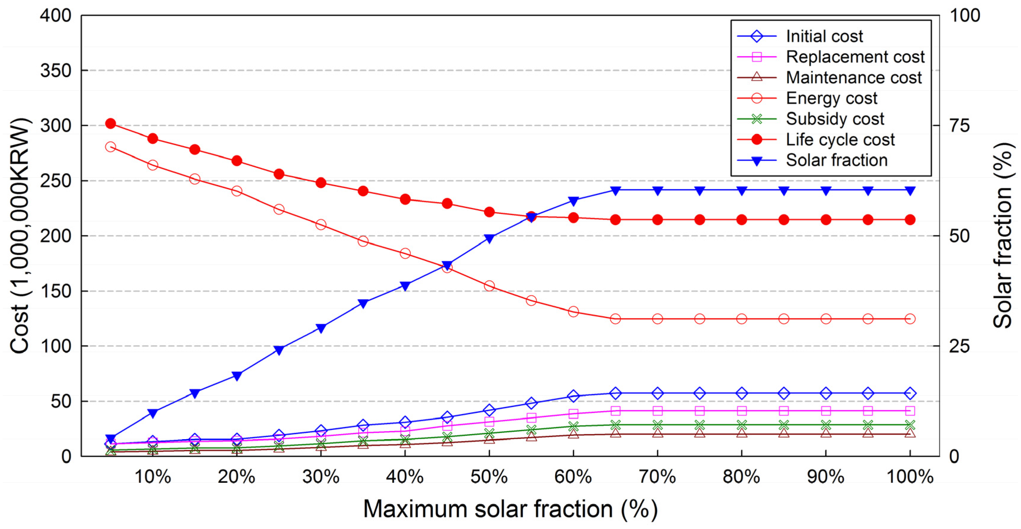
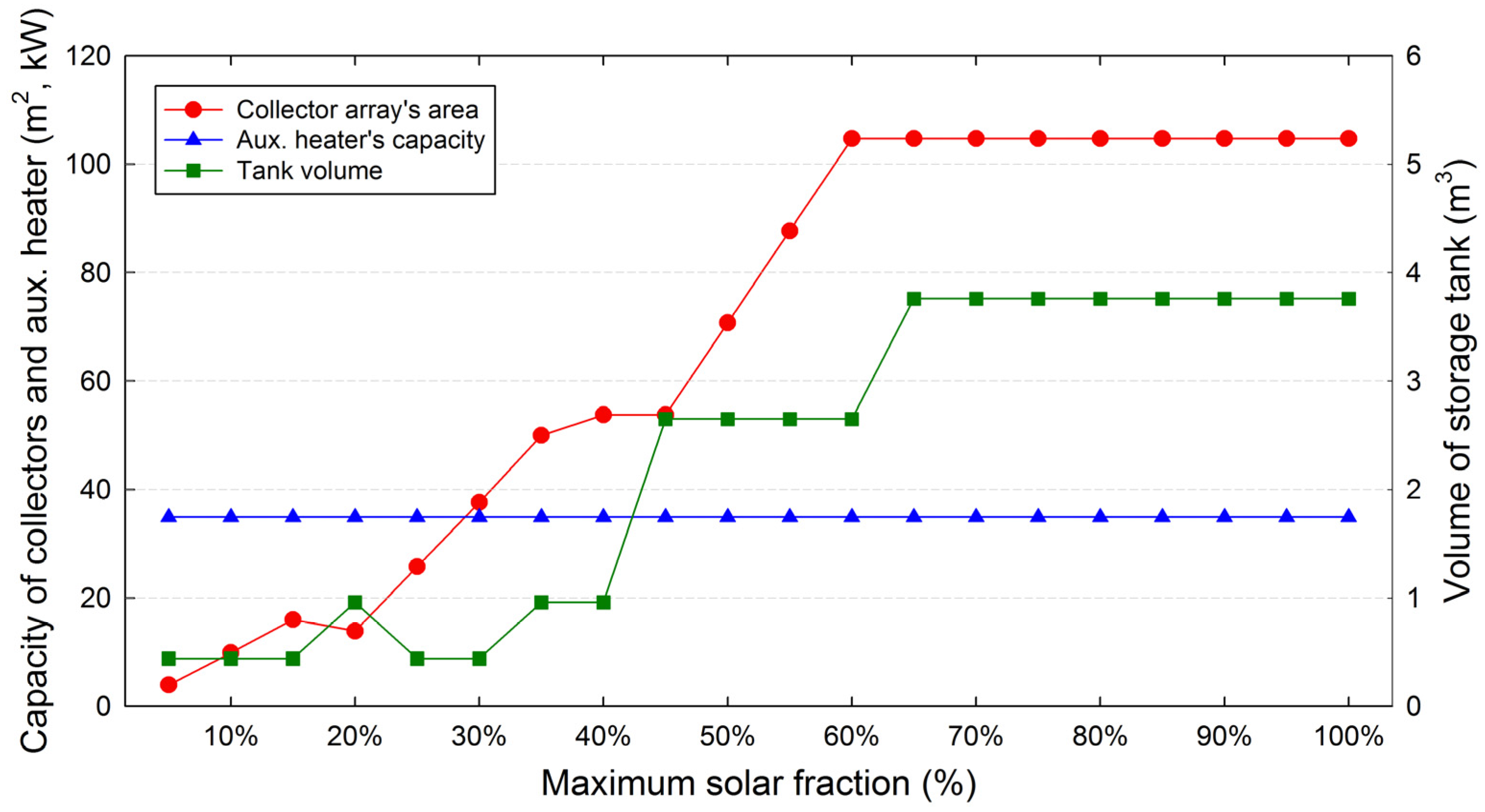
4.3. Effect According to Variation of the Maximum Solar Fraction

Given that the minimum solar fraction is set 0% and the maximum solar fraction is increased to 100% in 5% increments, variation in the LCC and solar fraction of the optimal SWH systems at each maximum solar fraction is shown in Figure 6. The results of the optimization design for the SWH systems with the minimum LCC for the different maximum solar fractions are given in Table 7. For the given design parameters and constraint conditions considered in this paper, the global optimum SWH system is observed at a LCC of 241.7 million KRW and at a solar fraction of 60.42% in the case of a maximum solar fraction of 65% and is the same as that of the base case in Section 4.2.

From Figure 6 and Table 7, for the SWH systems with a lower than maximum solar fraction of 65%, it can be seen that increasing the solar fraction leads to an increase in the equipment cost and a decrease in the energy cost. Note that satisfying the higher solar fraction means an increase in the capacity of the SWH system and the equipment cost represents a cost obtained by subtracting the subsidy cost from the sum of the initial, maintenance, and replacement costs. That is, for these SWH systems, the decrease in the energy cost due to the reduced fossil fuel consumption is larger than the increase in the equipment cost caused by increasing the capacity of the SWH system. Thus, the optimum design with the reduced LCC can be obtained by increasing the solar fraction of the SWH system until the maximum solar fraction reaches 65%. However, for the SWH systems with a higher maximum solar fraction of 70%, the proposed method derives the same optimal design as the case for the maximum solar fraction of 65% because the reduction in the energy cost is smaller than the increase in the equipment cost. Therefore, a trade-off between the equipment cost and the energy cost results in an optimal design of the SWH system that yields the minimum LCC.

Figure 6. Variation of costs and solar fractions at the different maximum solar fractions.

Figure 6. Variation of costs and solar fractions at the different maximum solar fractions.

Table 7. Characteristics of the optimal SWH systems for the different maximum solar fractions.

Parameter	Maximum Solar Fraction
	5%	10%	15%	20%	25%	30%	35%	40%	45%	50%	55%	60%	65%
$T_{coll}$ (–)	3	3	0	3	3	3	2	4	4	4	4	4	4
$N_{coll}$ (ea.)	2	5	8	7	13	19	25	19	19	25	31	37	37
$T_{tank}$ (–)	0	0	0	1	0	0	1	1	3	3	3	3	4
$T_{aux}$ (–)	4	4	4	4	4	4	4	4	4	4	4	4	4
$N_{aux}$ (ea.)	1	1	1	1	1	1	1	1	1	1	1	1	1
$A_{c,tot}$ (m2)	3.96	9.90	16.00	13.86	25.74	37.62	50	53.77	53.77	70.75	87.73	104.71	104.71
$V_s$ (m3)	0.44	0.44	0.44	0.96	0.44	0.44	0.96	0.96	2.65	2.65	2.65	2.65	3.76
$Q_{aux,tot}$ (kW)	34.89	34.89	34.89	34.89	34.89	34.89	34.89	34.89	34.89	34.89	34.89	34.89	34.89
$A_{c,ins}$ (m2)	7.4	18.4	29.7	25.7	47.8	69.8	92.7	99.8	99.8	131.3	162.8	194.3	194.3
$Q_{L,peak}$ (kW)	27.35	27.35	27.35	27.35	27.35	27.35	27.35	27.35	27.35	27.35	27.35	27.35	27.35
$Q_{L,year}$ (kWh/year)	60,218	60,218	60,218	60,218	60,218	60,218	60,218	60,218	60,218	60,218	60,218	60,218	60,218
$Q_{Ts}$ (kWh/year)	2462	5994	8740	11,159	14,698	17,754	21,185	23,695	26,625	30,374	33,440	35,901	37,332
$Q_l$ (kWh/year)	−57	−19	7	49	68	98	165	200	375	455	524	583	752
$Q_d$ (kWh/year)	0	0	0	0	0	3	1	7	0	0	5	21	4
$Q_{Ls}$ (kWh/year)	2523	6013	8731	11,103	14,624	17,622	20,986	23,385	26,195	29,848	32,744	34,966	36,386
$Q_{aux}$ (kWh/year)	57,695	54,205	51,487	49,115	45,594	42,596	39,232	36,833	34,023	30,370	27,474	25,252	23,832
$F_{LNG}$ (m3/year)	6083	5715	5428	5186	4810	4497	4154	3904	3623	3244	2940	2704	2562
$F_{ELE}$ (kWh/year)	142	186	335	354	516	632	799	909	892	1076	1260	1425	1413
$F_S$ (%)	4.19	9.99	14.50	18.44	24.28	29.26	34.85	38.83	43.50	49.56	54.37	58.06	60.42
$C_I$ (1000 KRW)	11,335	13,441	15,339	15,560	19,057	23,269	28,359	30,900	35,548	41,944	48,340	54,736	57,238
$C_M$ (1000 KRW)	3986	4727	5394	5472	6702	8183	9973	10,867	12,501	14,750	17,000	19,249	20,129
$C_R$ (1000 KRW)	11,444	12,630	13,699	14,188	15,793	18,165	21,395	22,826	27,812	31,414	35,016	38,618	41,302
$C_E$ (1000 KRW)	280,705	264,059	251,502	240,506	223,934	210,091	195,048	184,011	171,145	154,502	141,301	131,163	124,616
$C_S$ (1000 KRW)	5668	6721	7670	7780	9529	11,635	14,179	15,450	17,774	20,972	24,170	27,368	28,619
$C_{LCC}$ (1000 KRW)	301,802	288,136	278,264	267,946	255,957	248,073	240,596	233,154	229,232	221,638	217,487	216,398	214,666

Table 7. Characteristics of the optimal SWH systems for the different maximum solar fractions.

Parameter	Maximum Solar Fraction
	5%	10%	15%	20%	25%	30%	35%	40%	45%	50%	55%	60%	65%
$T_{coll}$ (–)	3	3	0	3	3	3	2	4	4	4	4	4	4
$N_{coll}$ (ea.)	2	5	8	7	13	19	25	19	19	25	31	37	37
$T_{tank}$ (–)	0	0	0	1	0	0	1	1	3	3	3	3	4
$T_{aux}$ (–)	4	4	4	4	4	4	4	4	4	4	4	4	4
$N_{aux}$ (ea.)	1	1	1	1	1	1	1	1	1	1	1	1	1
$A_{c,tot}$ (m2)	3.96	9.90	16.00	13.86	25.74	37.62	50	53.77	53.77	70.75	87.73	104.71	104.71
$V_s$ (m3)	0.44	0.44	0.44	0.96	0.44	0.44	0.96	0.96	2.65	2.65	2.65	2.65	3.76
$Q_{aux,tot}$ (kW)	34.89	34.89	34.89	34.89	34.89	34.89	34.89	34.89	34.89	34.89	34.89	34.89	34.89
$A_{c,ins}$ (m2)	7.4	18.4	29.7	25.7	47.8	69.8	92.7	99.8	99.8	131.3	162.8	194.3	194.3
$Q_{L,peak}$ (kW)	27.35	27.35	27.35	27.35	27.35	27.35	27.35	27.35	27.35	27.35	27.35	27.35	27.35
$Q_{L,year}$ (kWh/year)	60,218	60,218	60,218	60,218	60,218	60,218	60,218	60,218	60,218	60,218	60,218	60,218	60,218
$Q_{Ts}$ (kWh/year)	2462	5994	8740	11,159	14,698	17,754	21,185	23,695	26,625	30,374	33,440	35,901	37,332
$Q_l$ (kWh/year)	−57	−19	7	49	68	98	165	200	375	455	524	583	752
$Q_d$ (kWh/year)	0	0	0	0	0	3	1	7	0	0	5	21	4
$Q_{Ls}$ (kWh/year)	2523	6013	8731	11,103	14,624	17,622	20,986	23,385	26,195	29,848	32,744	34,966	36,386
$Q_{aux}$ (kWh/year)	57,695	54,205	51,487	49,115	45,594	42,596	39,232	36,833	34,023	30,370	27,474	25,252	23,832
$F_{LNG}$ (m3/year)	6083	5715	5428	5186	4810	4497	4154	3904	3623	3244	2940	2704	2562
$F_{ELE}$ (kWh/year)	142	186	335	354	516	632	799	909	892	1076	1260	1425	1413
$F_S$ (%)	4.19	9.99	14.50	18.44	24.28	29.26	34.85	38.83	43.50	49.56	54.37	58.06	60.42
$C_I$ (1000 KRW)	11,335	13,441	15,339	15,560	19,057	23,269	28,359	30,900	35,548	41,944	48,340	54,736	57,238
$C_M$ (1000 KRW)	3986	4727	5394	5472	6702	8183	9973	10,867	12,501	14,750	17,000	19,249	20,129
$C_R$ (1000 KRW)	11,444	12,630	13,699	14,188	15,793	18,165	21,395	22,826	27,812	31,414	35,016	38,618	41,302
$C_E$ (1000 KRW)	280,705	264,059	251,502	240,506	223,934	210,091	195,048	184,011	171,145	154,502	141,301	131,163	124,616
$C_S$ (1000 KRW)	5668	6721	7670	7780	9529	11,635	14,179	15,450	17,774	20,972	24,170	27,368	28,619
$C_{LCC}$ (1000 KRW)	301,802	288,136	278,264	267,946	255,957	248,073	240,596	233,154	229,232	221,638	217,487	216,398	214,666

Figure 7 shows a variation in component sizes for the optimal SWH systems at the different maximum solar fractions. To satisfy the increased solar fractions, the capacity of the optimal SWH systems is increased by applying more solar collectors or a larger storage tank. However, an auxiliary heater of 34.89 kW was selected for all SWH systems because this device has the highest efficiency and economically meets the energy balance as a constraint among the eight models. It is interesting to note that the sizing of solar collectors and a storage tank does not increase linearly in proportion to each other because the proposed optimization method uses devices that are actually available in the marketplace, showing the different technical and economic characteristics, instead of increasing the component sizes in constant increments. It is also found that there are three methods for increasing the solar fraction. The first method is to increase the capacity of one of the solar collectors and a storage tank and to keep the other’s capacity with the same condition. The second method is to increase the capacity of one of two components while decreasing the capacity of the remaining component. The last method is to increase the capacity of both components. Therefore, the proposed method determines the optimal sizing of the SWH systems in the most economical way for these three methods.

Figure 7. Variation of component sizes at the different maximum solar fractions.

Figure 7. Variation of component sizes at the different maximum solar fractions.

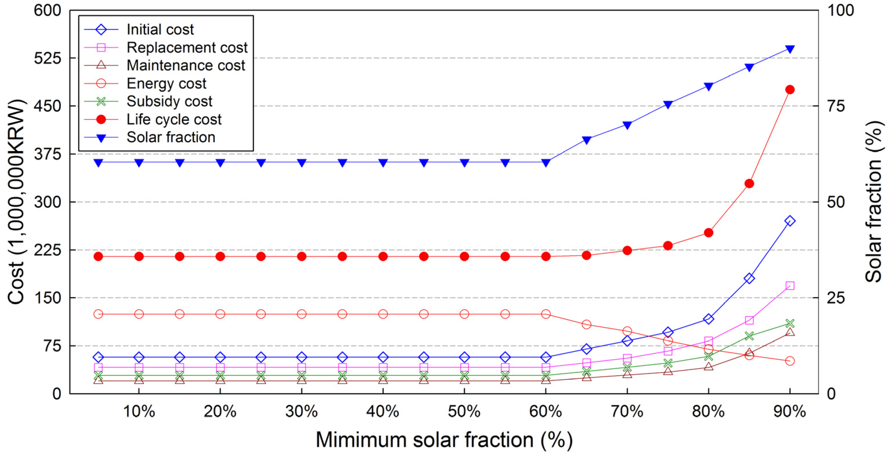
4.4. Effect According to Variation of the Minimum Solar Fraction

Figure 8 shows a variation in the LCC and solar fraction of the optimal SWH systems at each minimum solar fraction. Variation in component sizes for the different minimum solar fractions is also shown in Figure 9. Here, the minimum solar fraction is increased to 100% in 5% increments, and the maximum solar fraction is set 100%. The results of the optimization design for the SWH systems at the different minimum solar fractions are listed in Table 8. The configuration and sizing of the optimal SWH systems derived from the constraint condition set to the minimum solar fraction of 5%–60% are the same as that of the global optimum SWH system. Note that the SWH systems obtained from the constraint condition set to the minimum solar fraction of 85% and 90% are infeasible solutions because the installation area of the solar collectors for two system designs exceeded the maximum installable area as a constraint. However, this paper analyzed these two SWH systems along with other systems to evaluate the characteristics of the SWH systems according to variations in the solar fraction.

Figure 8. Variation of costs and solar fraction at the different minimum solar fractions.

Figure 8. Variation of costs and solar fraction at the different minimum solar fractions.

Figure 9. Variation of component sizes at the different minimum solar fractions.

Figure 9. Variation of component sizes at the different minimum solar fractions.

It may be observed from Table 8 that the energy performance of the optimal SWH systems changes according to the solar fraction. To improve the solar fraction of 5%, an additional energy of approximately 3000 MWh/year is supplied from a storage tank to the load in the SWH systems with minimum solar fractions of 65%–90%. However, the average annual energy inputted to a storage tank is approximately 4700 MWh/year for six SWH systems. In the SWH systems at the high solar fraction such as the minimum solar fractions of 85% and 90%, those energies of 7662 MWh/year and 6443 MWh/year are considerably larger than the average amount. That is, by applying more solar collectors or a larger storage tank, more energy than the amount of energy required to increase the solar fraction is introduced into a storage tank and is used to keep the storage tank temperature high for a long time. In addition, the high temperature of a storage tank increases the annual heat loss to the ambient air and annual discharged heat to avoid overheating. It may also be observed from Figure 8 and Table 8 that the LCC of the systems raises significantly because the increase in the equipment cost is considerably larger than the decrease in the energy cost. Compared to the global optimum SWH system, for the SWH systems with the minimum solar fractions of 65%, 70%, 75%, and 80%, there are increases of 20%, 40%, 65% and 102% in the equipment cost and the decreases of 13%, 22%, 34%, and 44% in the energy cost, respectively. Furthermore, the LCC of the optimal SWH systems with the minimum solar fractions of 85% and 90% is approximately 30.40% and 88.78% higher than the LCC of the optimal SWH system with the minimum solar fraction of 80% only to increase to an additional solar fraction of 4.99% and 9.78%, respectively; therefore, increasing the solar fraction larger than that of the global optimum SWH system results in a reduction in the energetic and economic performance of the systems.

Table 8. Characteristics of the optimal SWH systems for the different minimum solar fractions.

Parameter	Minimum Soar Fraction
	60	65	70	75	80	85	90
$T_{coll}$ (–)	4	4	4	4	4	4	4
$N_{coll}$ (ea.)	37	49	61	67	79	145	223
$T_{tank}$ (–)	4	4	4	7	9	8	9
$T_{aux}$ (–)	4	4	4	4	4	4	4
$N_{aux}$ (ea.)	1	1	1	1	1	1	1
$A_{c,tot}$ (m2)	104.71	138.67	172.63	189.61	223.57	410.35	631.09
$V_s$ (m3)	3.76	3.76	3.76	6.21	9.58	6.92	9.58
$Q_{aux,tot}$ (kW)	34.89	34.89	34.89	34.89	34.89	34.89	34.89
$A_{c,ins}$ (m2)	194.3	257.3	320.3	351.8	414.8	761.3	1170.9
$Q_{L,peak}$ (kW)	27.35	27.35	27.35	27.35	27.35	27.35	27.35
$Q_{L,year}$ (kWh/year)	60,218	60,218	60,218	60,218	60,218	60,218	60,218
$Q_{Ts}$ (kWh/year)	37,332	41,410	44,318	47,618	51,206	58,867	65,290
$Q_l$ (kWh/year)	752	886	994	1138	1684	1922	2221
$Q_d$ (kWh/year)	4	36	78	49	43	402	607
$Q_{Ls}$ (kWh/year)	36,386	39,949	42,303	45,517	48,367	51,372	54,256
$Q_{aux}$ (kWh/year)	23,832	20,269	17,915	14,701	11,851	8846	5962
$F_{LNG}$ (m3/year)	2562	2181	1928	1595	1291	966	660
$F_{ELE}$ (kWh/year)	1413	1712	1986	2064	2279	3630	5053
$F_S$ (%)	60.42	66.34	70.25	75.59	80.32	85.31	90.10
$C_I$ (1000 KRW)	57,238	70,030	82,822	96,197	117,025	180,589	270,529
$C_M$ (1000 KRW)	20,129	24,628	29,126	33,830	41,155	63,508	95,137
$C_R$ (1000 KRW)	41,302	48,506	55,710	66,797	82,622	114,957	169,068
$C_E$ (1000 KRW)	124,616	108,296	97,765	82,838	69,716	59,867	51,207
$C_S$ (1000 KRW)	28,619	35,015	41,411	48,098	58,513	90,294	110,214
$C_{LCC}$ (1000 KRW)	214,666	216,445	224,012	231,564	252,005	328,627	475,727

Table 8. Characteristics of the optimal SWH systems for the different minimum solar fractions.

Parameter	Minimum Soar Fraction
	60	65	70	75	80	85	90
$T_{coll}$ (–)	4	4	4	4	4	4	4
$N_{coll}$ (ea.)	37	49	61	67	79	145	223
$T_{tank}$ (–)	4	4	4	7	9	8	9
$T_{aux}$ (–)	4	4	4	4	4	4	4
$N_{aux}$ (ea.)	1	1	1	1	1	1	1
$A_{c,tot}$ (m2)	104.71	138.67	172.63	189.61	223.57	410.35	631.09
$V_s$ (m3)	3.76	3.76	3.76	6.21	9.58	6.92	9.58
$Q_{aux,tot}$ (kW)	34.89	34.89	34.89	34.89	34.89	34.89	34.89
$A_{c,ins}$ (m2)	194.3	257.3	320.3	351.8	414.8	761.3	1170.9
$Q_{L,peak}$ (kW)	27.35	27.35	27.35	27.35	27.35	27.35	27.35
$Q_{L,year}$ (kWh/year)	60,218	60,218	60,218	60,218	60,218	60,218	60,218
$Q_{Ts}$ (kWh/year)	37,332	41,410	44,318	47,618	51,206	58,867	65,290
$Q_l$ (kWh/year)	752	886	994	1138	1684	1922	2221
$Q_d$ (kWh/year)	4	36	78	49	43	402	607
$Q_{Ls}$ (kWh/year)	36,386	39,949	42,303	45,517	48,367	51,372	54,256
$Q_{aux}$ (kWh/year)	23,832	20,269	17,915	14,701	11,851	8846	5962
$F_{LNG}$ (m3/year)	2562	2181	1928	1595	1291	966	660
$F_{ELE}$ (kWh/year)	1413	1712	1986	2064	2279	3630	5053
$F_S$ (%)	60.42	66.34	70.25	75.59	80.32	85.31	90.10
$C_I$ (1000 KRW)	57,238	70,030	82,822	96,197	117,025	180,589	270,529
$C_M$ (1000 KRW)	20,129	24,628	29,126	33,830	41,155	63,508	95,137
$C_R$ (1000 KRW)	41,302	48,506	55,710	66,797	82,622	114,957	169,068
$C_E$ (1000 KRW)	124,616	108,296	97,765	82,838	69,716	59,867	51,207
$C_S$ (1000 KRW)	28,619	35,015	41,411	48,098	58,513	90,294	110,214
$C_{LCC}$ (1000 KRW)	214,666	216,445	224,012	231,564	252,005	328,627	475,727

Meanwhile, it may be noted from Table 7 in Section 4.3 and Table 8 that the SWH system with the minimum solar fraction of 70% exhibits a better economic benefit and energy savings than the SWH systems with the maximum solar fraction of 5%–45%. Thus, an increase in the solar fraction does not necessarily indicate a reduction in the economic benefit. These simulation results using the proposed method show that economic feasibility is converted based on the solar fraction of the global optimum SWH system. Therefore, it is necessary to design the configuration and sizing of a SWH system using the optimization method based on the economic criterion.

5. Conclusions

The optimization design for a SWH system is a complicated process that uses mathematical models with many meteorological, technical, and economic variables. Thus, it has been difficult for traditional design techniques in the past to obtain satisfactory results within a reasonable computation time. In this paper, a GA has been employed to optimize the configuration and sizing of the SWH system on the basis of LCC. Through a numerical example of the SWH system for an office building in Incheon, South Korea, the effectiveness of the proposed method has been demonstrated. It was found that the LCC of the SWH system decreases first. Then, its decreasing speed becomes slow gradually and reaches the minimum cost. Finally, it increases sharply with the increase in capacity and solar fraction. This indicates that the global optimum SWH system was derived from the optimum solar fraction to maximize the economic benefits under given design conditions. Therefore, it could be helpful to determine the optimal configuration and sizing of the SWH system by comparing the feasible designs obtained by using the proposed method instead of simply adjusting the solar fraction depending only on the designer’s experience and intuition. Future work includes a further improvement of the proposed method to reflect the parameters, such as the slope and azimuth of collectors, flow rates on the hot and cold side of the heat exchanger, and operation conditions that affect the energetic and economic performance of the SWH system.

References

1. Wang, Z.; Yang, W.; Qiu, F.; Zhang, X.; Zhao, X. Solar water heating: From theory, application, marketing and research. Renew. Sustain. Energy Rev. 2015, 41, 68–84. [Google Scholar] [CrossRef]
2. Balusamy, T.; Sadhishkumar, S. Performance improvement in solar water heating systems—A review. Renew. Sustain. Energy Rev. 2014, 37, 191–198. [Google Scholar]
3. Islam, M.R.; Sumathy, K.; Khan, S.U. Solar water heating systems and their market trends. Renew. Sustain. Energy Rev. 2013, 17, 1–25. [Google Scholar] [CrossRef]
4. Renewable Energy Policy Network. Renewable Energy 2010: Key Facts and Figures for Decision Makers. Global Status Report. Available online: http://www.ren21.net/gsr (accessed on 10 July 2015).
5. Kulkarni, G.N.; Kedare, S.B.; Bandyopadhyay, S. Determination of design space and optimization of solar water heating systems. Sol. Energy 2007, 81, 958–968. [Google Scholar] [CrossRef]
6. Hottel, H.C.; Whillier, A. Evaluation of Flat-Plate Collector Performance; University of Arizona Press: Tucson, AZ, USA, 1958. [Google Scholar]
7. Klein, S.A. Calculation of flat-plate collector utilizability. Sol. Energy 1978, 21, 393–402. [Google Scholar] [CrossRef]
8. Klein, S.A.; Beckman, W.A.; Duffie, J.A. A design procedure for solar heating systems. Sol. Energy 1976, 18, 113–127. [Google Scholar] [CrossRef]
9. Klein, S.A.; Beckman, W.A. A general design method for closed-loop solar energy systems. Sol. Energy 1979, 22, 269–282. [Google Scholar] [CrossRef]
10. Yan, C.; Wang, S.; Ma, Z.; Shi, W. A simplified method for optimal design of solar water heating systems based on life-cycle energy analysis. Renew. Energy 2015, 74, 271–278. [Google Scholar] [CrossRef]
11. Klein, S.A.; Cooper, P.I.; Freeman, T.L.; Beekman, D.L.; Beckman, W.A.; Duffie, J.A. A method of simulation of solar processes and its application. Sol. Energy 1975, 17, 29–37. [Google Scholar] [CrossRef]
12. Lund, P.D.; Peltola, S.S. SOLCHIPS—A fast pre-design and optimization tool for solar heating with seasonal storage. Sol. Energy 1992, 48, 291–300. [Google Scholar] [CrossRef]
13. Matrawy, K.K.; Farkas, I. New technique for short term storage sizing. Renew. Energy 1997, 11, 129–141. [Google Scholar] [CrossRef]
14. Loomans, M.; Visser, H. Application of the genetic algorithm for optimization of large solar hot water systems. Sol. Energy 2002, 72, 427–439. [Google Scholar] [CrossRef]
15. Krause, M.; Vajen, K.; Wiese, F.; Ackermann, H. Investigation on optimizing large solar thermal systems. Sol. Energy 2002, 73, 217–225. [Google Scholar] [CrossRef]
16. Kalogirou, S.A. Optimization of solar systems using artificial neural-networks and genetic algorithms. Appl. Energy 2004, 77, 383–405. [Google Scholar] [CrossRef]
17. Kulkarni, G.N.; Kedare, S.B.; Bandyopadhyay, S. Design of solar thermal systems utilizing pressurized hot water storage for industrial applications. Sol. Energy 2008, 82, 686–699. [Google Scholar] [CrossRef]
18. Kim, Y.D.; Thu, K.; Bhatia, H.K.; Bhatia, C.S.; Ng, K.C. Thermal analysis and performance optimization of a solar hot water plant with economic evaluation. Sol. Energy 2012, 86, 1378–1395. [Google Scholar] [CrossRef]
19. Atia, D.M.; Fahmy, F.H.; Ahmed, N.M.; Dorrah, H.T. Optimal sizing of a solar water heating system based on a genetic algorithm for an aquaculture system. Math. Comput. Model. 2012, 55, 1436–1449. [Google Scholar] [CrossRef]
20. Bornatico, R.; Pfeiffer, M.; Witzig, A.; Guzzella, L. Optimal sizing of a solar thermal building installation using particle swarm optimization. Energy 2012, 41, 31–37. [Google Scholar] [CrossRef]
21. Cheng Hin, J.N.; Zmeureanu, R. Optimization of a residential solar combisystem for minimum life cycle cost, energy use and exergy destroyed. Sol. Energy 2014, 100, 102–113. [Google Scholar] [CrossRef]
22. Kusyy, O.; Kuethe, S.; Vajen, K. Simulation-based optimization of a solar water heating system by a hybrid genetic-binary search algorithm. In Proceedings of the 2010 Xvth International Seminar/Workshop on Direct and Inverse Problems of Electromagnetic and Acoustic Wave Theory (DIPED), Tbilisi, GA, USA, 27–30 September 2010.
23. Duffie, J.A.; Beckman, W.A. Solar Engineering of Thermal Processes, 3rd ed.; Willey: Hoboken, NJ, USA, 2006. [Google Scholar]
24. Choi, D.S.; Ko, M.J. Optimization design for a solar water heating system using the genetic algorithm. Int. J. Appl. Eng. Res. 2015, 10, 27031–27042. [Google Scholar]
25. Kanpur Genetic Algorithms Laboratory. Available online: http://www.iitk.ac.in/kangal/codes.shtml (accessed on 29 January 2015).
26. Ko, M.J.; Kim, Y.S.; Chung, M.H.; Jeon, H.C. Multi-objective optimization design for a hybrid energy system using the genetic algorithm. Energies 2015, 8, 2924–2949. [Google Scholar] [CrossRef]
27. National Renewable Energy Laboratory. U.S. Department of Energy Commercial Reference Building Models of the National Building Stock. Available online: http://www.nrel.gov/docs/fy11osti/46861.pdf (accessed on 29 January 2015).