
A Tabu Search Algorithm for the Power System Islanding Problem


Abstract
:1. Introduction


2. Related Work
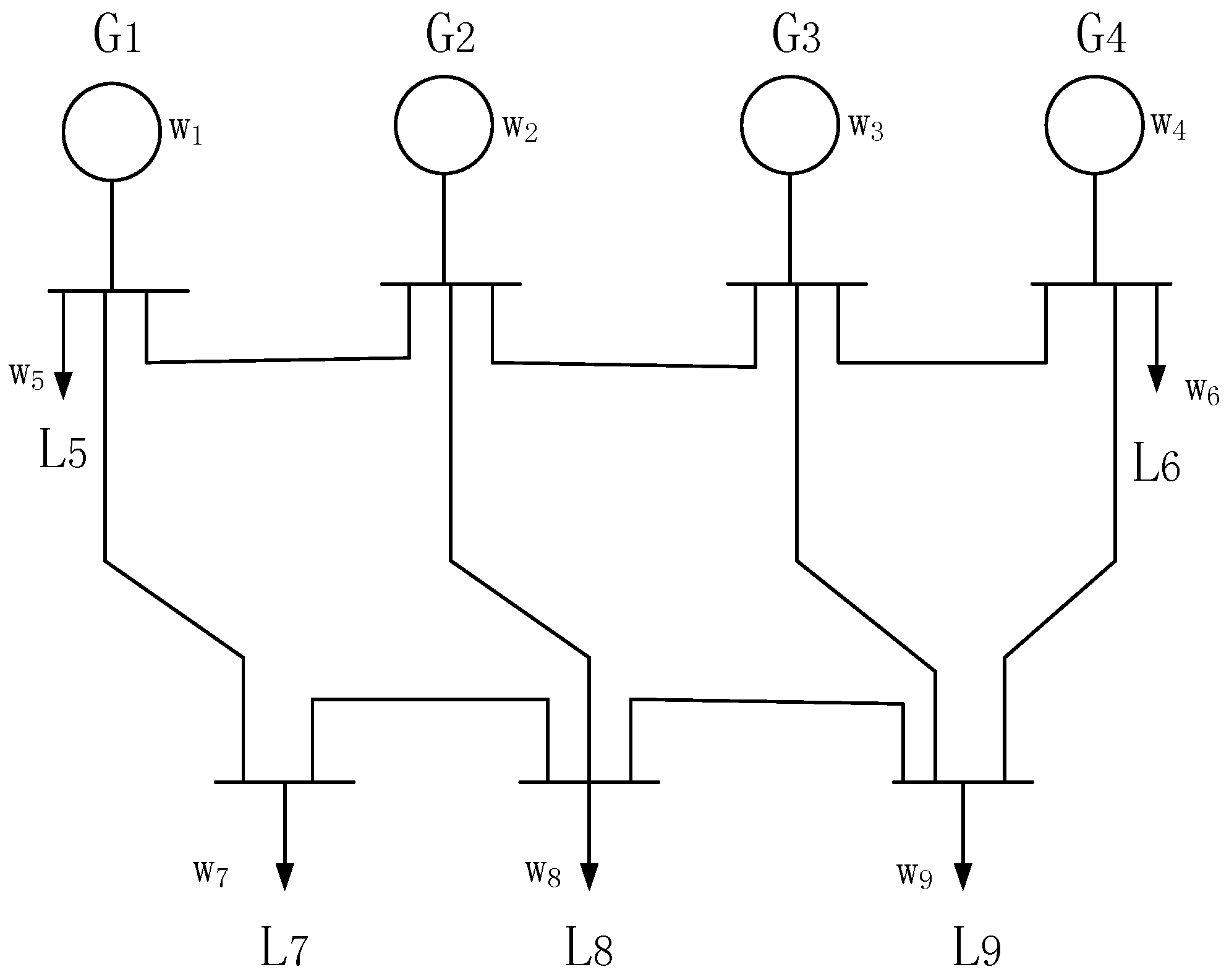
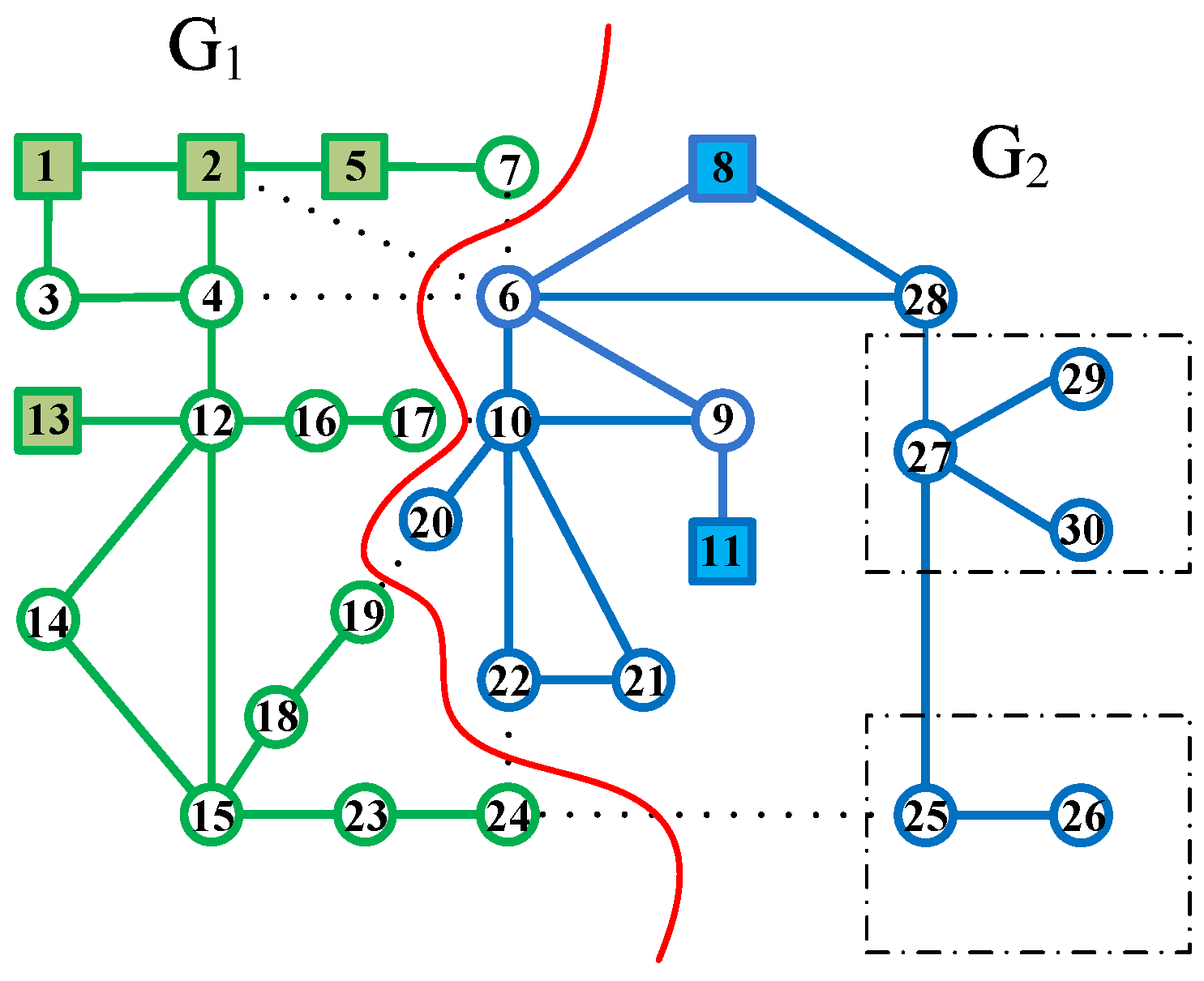
3. Problem Description
4. Tabu Search
4.1. Input Data

4.2. Initial Solution


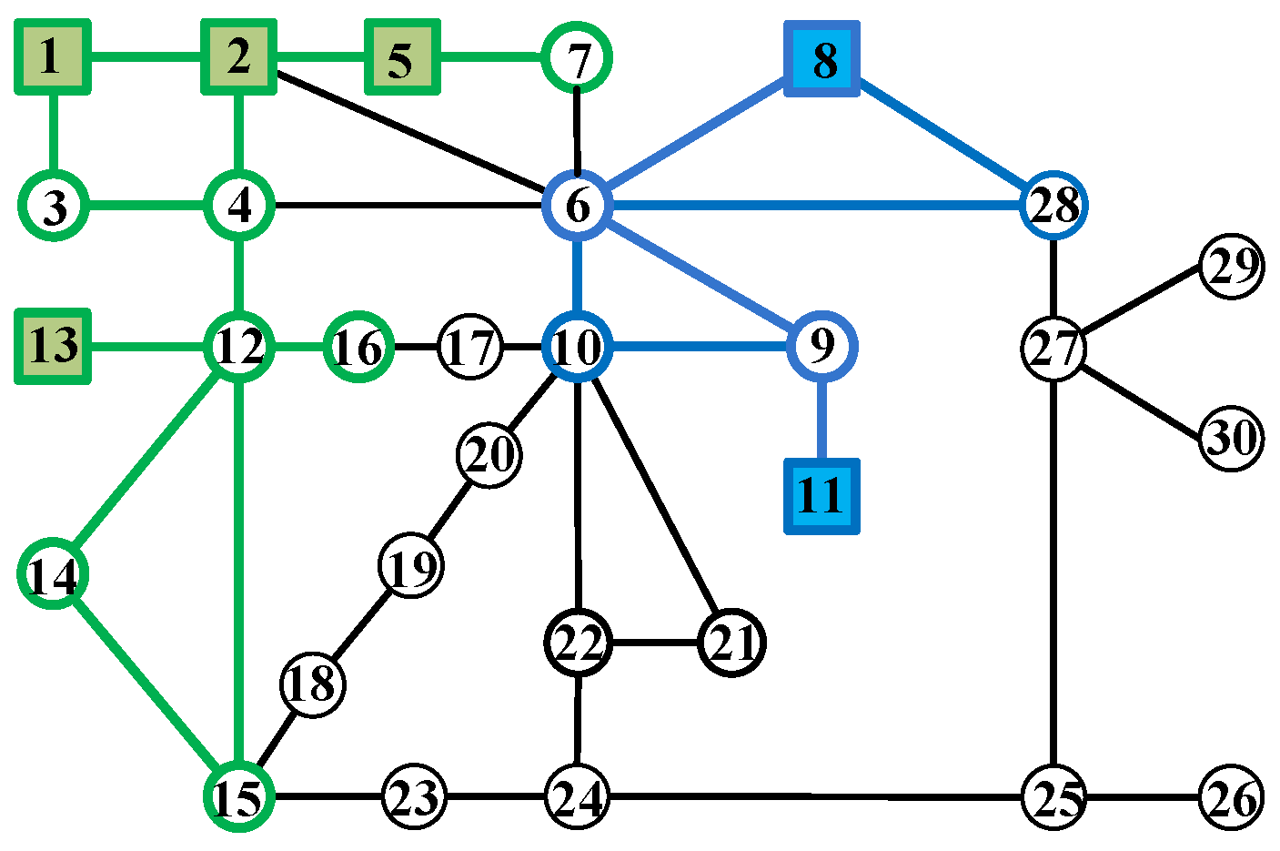

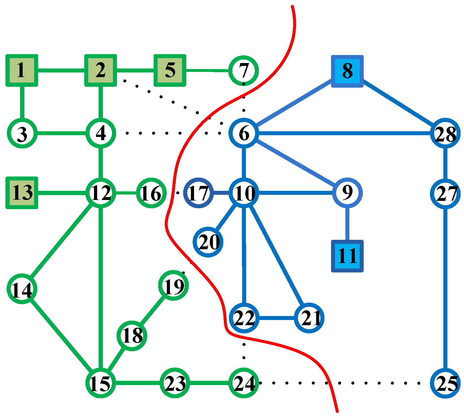
4.3. Neighborhood
4.4. Tabu List, Aspiration and Termination
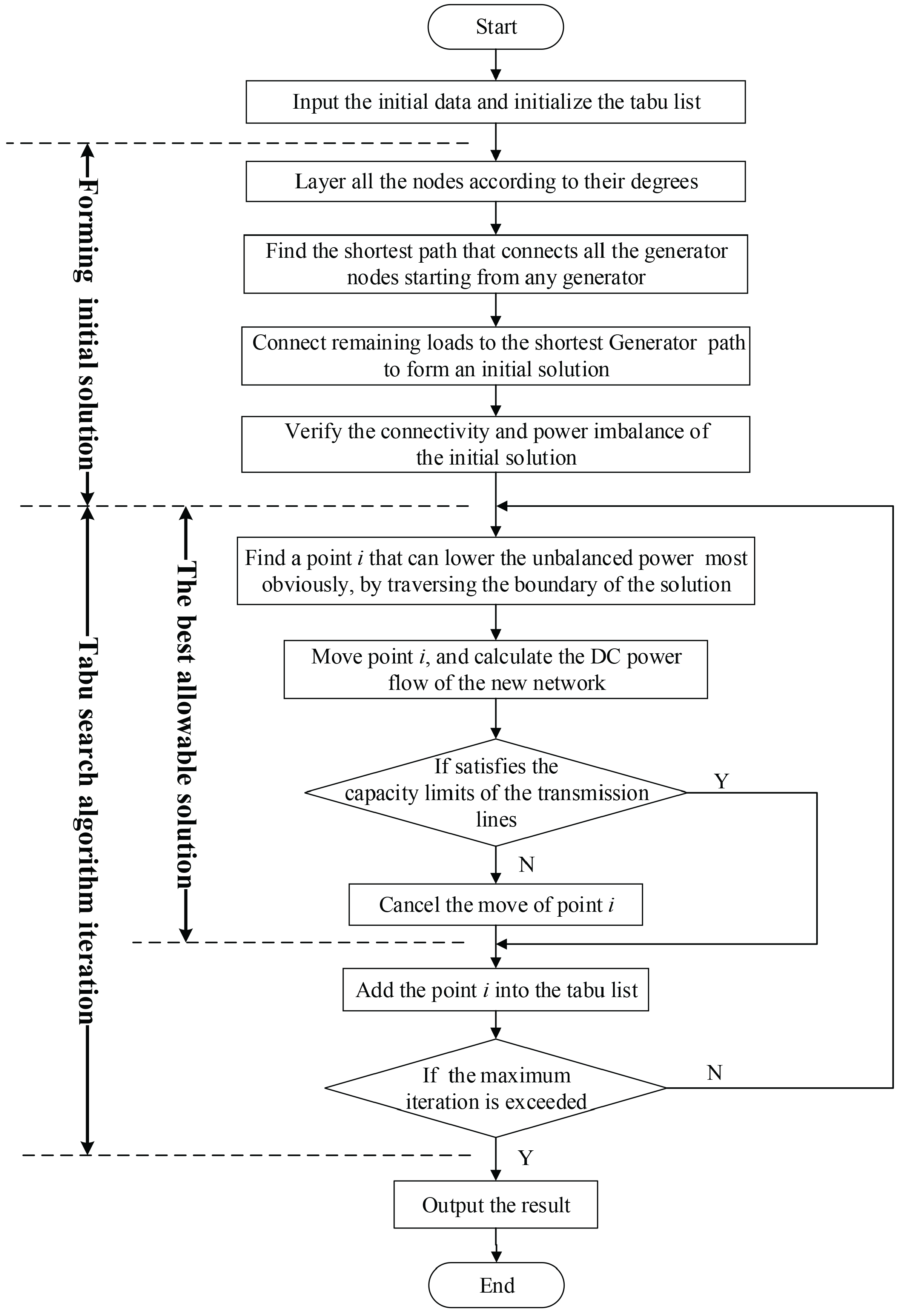
4.5. The Framework of the Algorithm
| Algorithm 1 The tabu search algorithm. |
|
5. Experimental Results
5.1. Benchmark Instances

| Name | # Edges | # Generation nodes | # Load nodes | Total generation power (Mega Watt) | Total load power (Mega Watts) |
|---|---|---|---|---|---|
| ieee118 | 186 | 19 | 99 | 3,966.93 | −3966.93 |
| sop2737 | 3506 | 185 | 2552 | 10,391.16 | −10,391.16 |
| wop2746 | 3514 | 336 | 2410 | 17,037.25 | −17,037.25 |
| wp3012 | 3572 | 292 | 2720 | 24,487.14 | −24,487.14 |
| sp3120 | 3693 | 241 | 2879 | 19,713.23 | −19,713.23 |
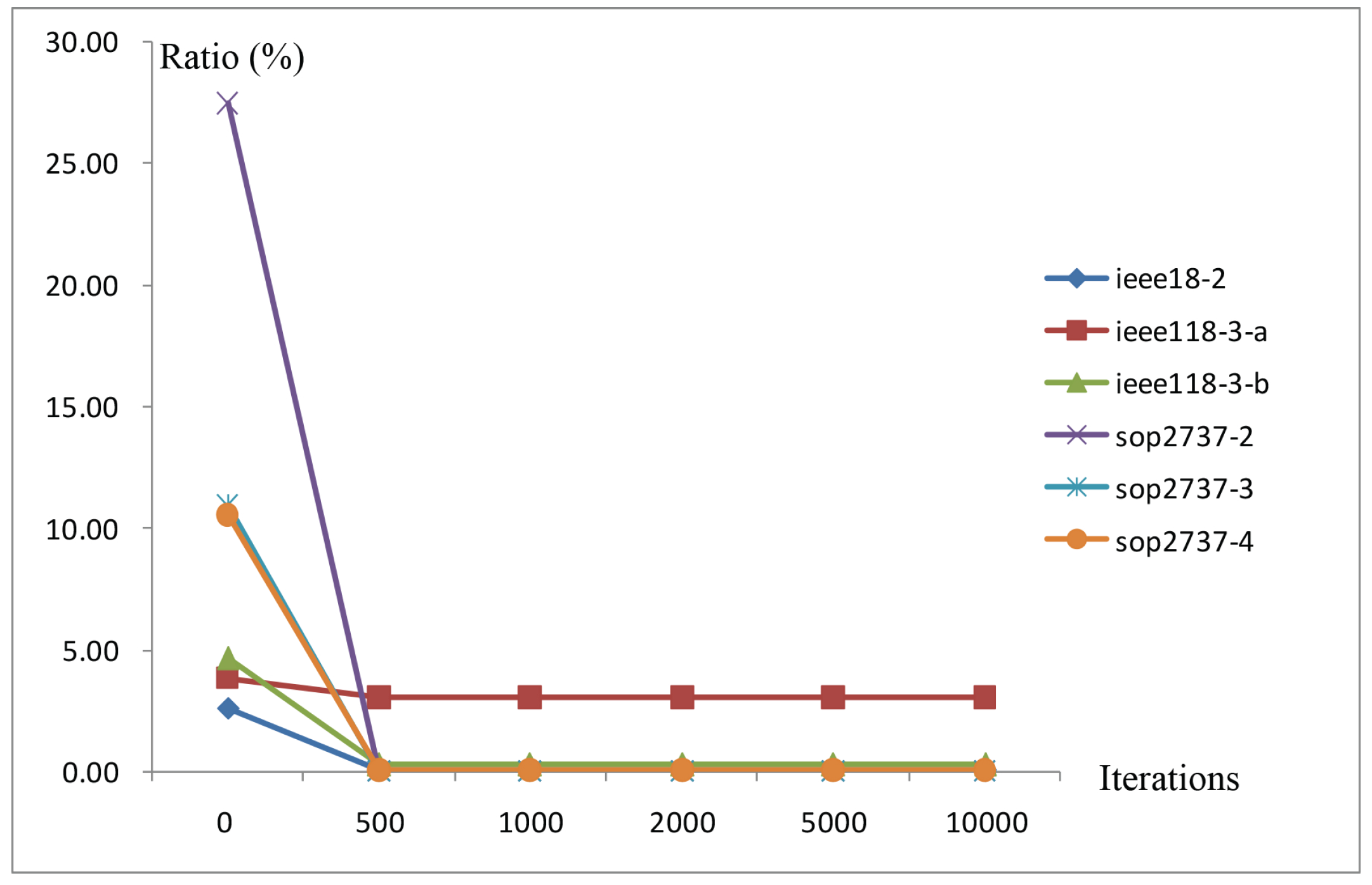
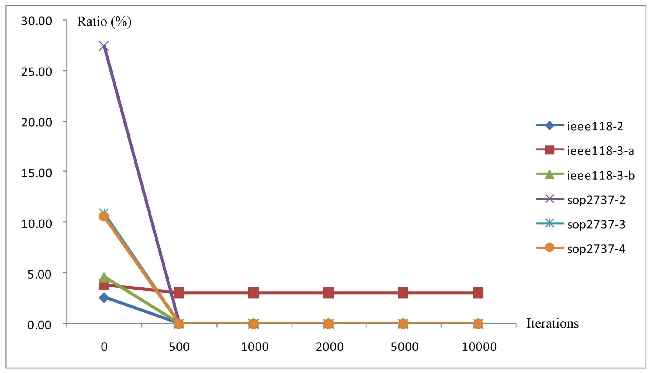
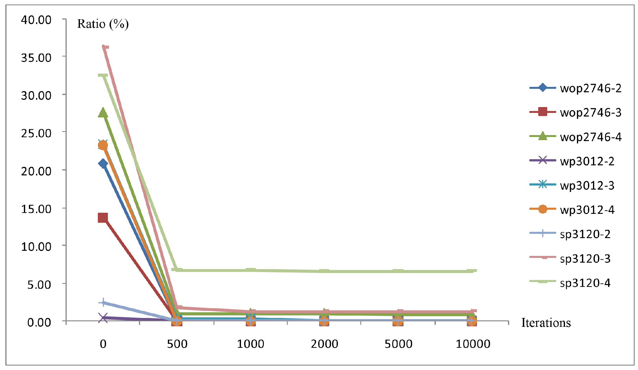
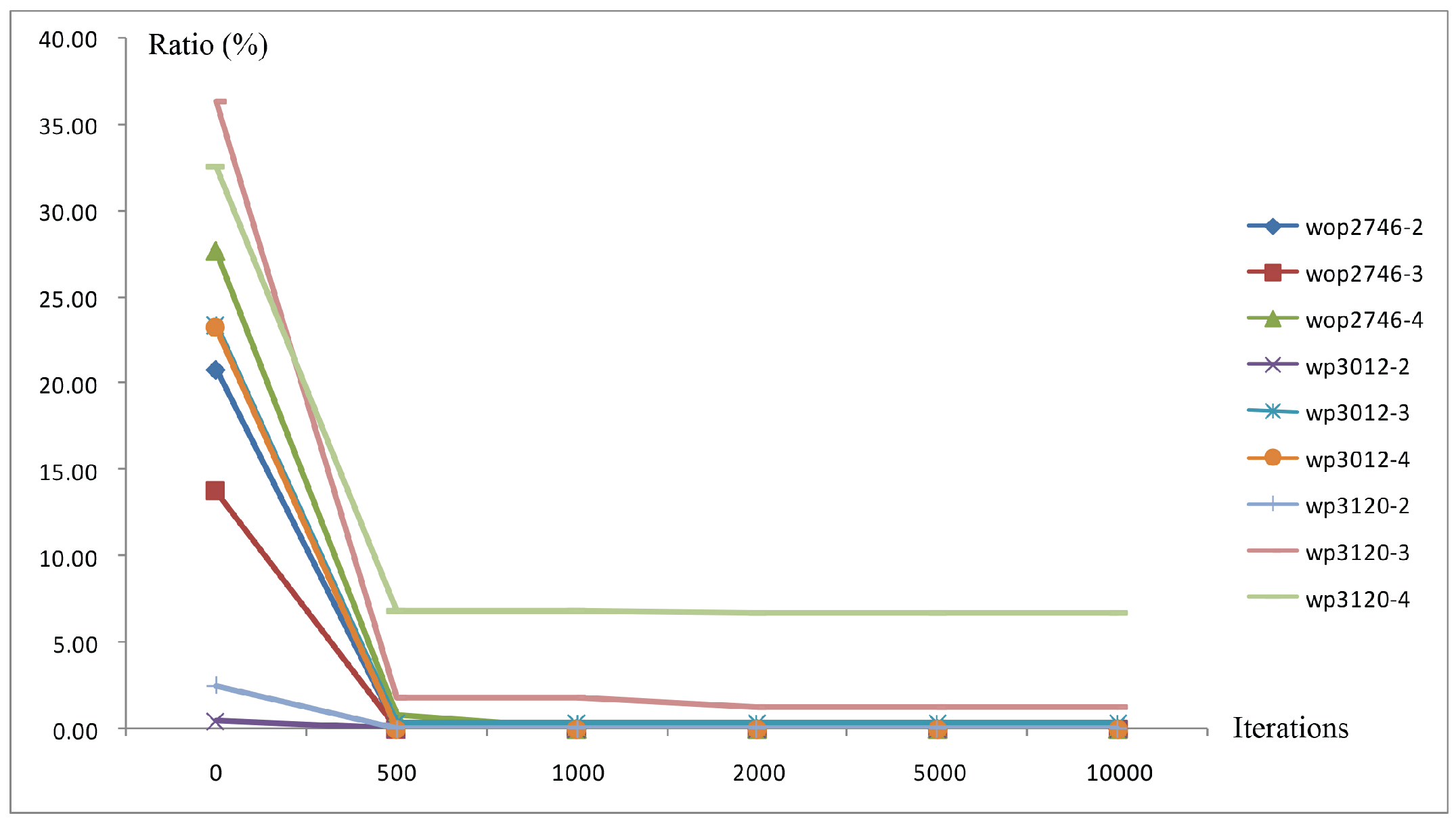
5.2. Results and Analyses
| Instance | 0 iterations | 500 iterations | 1000 iterations | 2000 iterations | 5000 iterations | 10,000 iterations | ||||||||||
|---|---|---|---|---|---|---|---|---|---|---|---|---|---|---|---|---|
| Ratio (%) | Time (s) | Ratio (%) | Time (s) | Ratio (%) | Time (s) | Ratio (%) | Time (s) | Ratio (%) | Time (s) | Ratio (%) | ||||||
| ieee118-2 | 2.59 | 0.004 | 0.00 | 0.008 | 0.00 | 0.016 | 0.00 | 0.042 | 0.00 | 0.087 | 0.00 | |||||
| ieee118-3-a | 3.83 | 0.003 | 3.01 | 0.005 | 3.01 | 0.011 | 3.01 | 0.028 | 3.01 | 0.055 | 3.01 | |||||
| ieee118-3-b | 4.60 | 0.001 | 0.26 | 0.016 | 0.26 | 0.015 | 0.26 | 0.032 | 0.26 | 0.062 | 0.26 | |||||
| sop2737-2 | 27.45 | 0.305 | 0.00 | 0.566 | 0.00 | 1.107 | 0.00 | 2.708 | 0.00 | 5.385 | 0.00 | |||||
| sop2737-3 | 10.90 | 0.131 | 0.00 | 0.255 | 0.00 | 0.495 | 0.00 | 1.231 | 0.00 | 2.448 | 0.00 | |||||
| sop2737-4 | 10.55 | 0.169 | 0.00 | 0.367 | 0.00 | 0.764 | 0.00 | 1.963 | 0.00 | 3.949 | 0.00 | |||||
| wop2746-2 | 20.83 | 0.259 | 0.00 | 0.529 | 0.00 | 1.084 | 0.00 | 2.695 | 0.00 | 5.397 | 0.00 | |||||
| wop2746-3 | 13.72 | 0.190 | 0.01 | 0.365 | 0.01 | 0.592 | 0.01 | 1.268 | 0.01 | 2.357 | 0.01 | |||||
| wop2746-4 | 27.68 | 0.236 | 0.75 | 0.482 | 0.01 | 0.842 | 0.01 | 1.901 | 0.01 | 3.639 | 0.01 | |||||
| wp3012-2 | 0.43 | 0.122 | 0.01 | 0.289 | 0.01 | 0.669 | 0.01 | 1.970 | 0.01 | 4.112 | 0.01 | |||||
| wp3012-3 | 23.39 | 0.295 | 0.33 | 0.692 | 0.33 | 1.469 | 0.33 | 3.814 | 0.33 | 7.706 | 0.33 | |||||
| wp3012-4 | 23.26 | 0.099 | 0.01 | 0.207 | 0.01 | 0.426 | 0.01 | 1.100 | 0.01 | 2.201 | 0.01 | |||||
| sp3120-2 | 2.49 | 0.150 | 0.00 | 0.275 | 0.00 | 0.552 | 0.00 | 1.374 | 0.00 | 2.710 | 0.00 | |||||
| sp3120-3 | 36.38 | 0.308 | 1.87 | 0.668 | 1.83 | 1.352 | 1.29 | 3.100 | 1.29 | 6.007 | 1.29 | |||||
| sp3120-4 | 32.56 | 0.189 | 6.86 | 0.440 | 6.86 | 0.983 | 6.73 | 3.123 | 6.73 | 6.597 | 6.73 | |||||
| Average | 16.04 | 0.164 | 0.87 | 0.344 | 0.82 | 0.692 | 0.78 | 1.757 | 0.78 | 3.514 | 0.78 | |||||
| Instance | 0 iterations | 500 iterations | 1000 iterations | 2000 iterations | 5000 iterations | 10,000 iterations | ||||||||||
|---|---|---|---|---|---|---|---|---|---|---|---|---|---|---|---|---|
| Ratio (%) | Time (s) | Ratio (%) | Time (s) | Ratio (%) | Time (s) | Ratio (%) | Time (s) | Ratio (%) | Time (s) | Ratio (%) | ||||||
| ieee118-2 | 2.59 | 0.003 | 0.00 | 0.008 | 0.00 | 0.014 | 0.00 | 0.035 | 0.00 | 0.071 | 0.00 | |||||
| ieee118-3-a | 3.83 | 0.002 | 3.01 | 0.004 | 3.01 | 0.006 | 3.01 | 0.016 | 3.01 | 0.032 | 3.01 | |||||
| ieee118-3-b | 4.60 | 0.001 | 0.07 | 0.001 | 0.05 | 0.016 | 0.05 | 0.031 | 0.04 | 0.062 | 0.04 | |||||
| sop2737-2 | 27.45 | 0.272 | 0.00 | 0.488 | 0.00 | 0.922 | 0.00 | 2.187 | 0.00 | 4.298 | 0.00 | |||||
| sop2737-3 | 10.90 | 0.137 | 0.00 | 0.264 | 0.00 | 0.520 | 0.00 | 1.338 | 0.00 | 2.684 | 0.00 | |||||
| sop2737-4 | 10.55 | 0.171 | 0.00 | 0.400 | 0.00 | 0.806 | 0.00 | 2.085 | 0.00 | 4.207 | 0.00 | |||||
| wop2746-2 | 20.83 | 0.275 | 0.00 | 0.591 | 0.00 | 1.201 | 0.00 | 3.050 | 0.00 | 6.142 | 0.00 | |||||
| wop2746-3 | 13.72 | 0.214 | 0.01 | 0.445 | 0.01 | 0.889 | 0.01 | 2.284 | 0.01 | 4.694 | 0.01 | |||||
| wop2746-4 | 27.68 | 0.230 | 1.01 | 0.463 | 1.01 | 0.915 | 1.01 | 2.313 | 0.87 | 6.500 | 0.87 | |||||
| wp3012-2 | 0.43 | 0.193 | 0.01 | 0.432 | 0.01 | 0.878 | 0.01 | 2.241 | 0.01 | 4.441 | 0.01 | |||||
| wp3012-3 | 23.39 | 0.288 | 0.33 | 0.681 | 0.33 | 1.191 | 0.01 | 2.526 | 0.01 | 4.760 | 0.01 | |||||
| wp3012-4 | 23.26 | 0.106 | 0.01 | 0.211 | 0.01 | 0.435 | 0.01 | 1.076 | 0.01 | 2.164 | 0.01 | |||||
| sp3120-2 | 2.49 | 0.225 | 0.00 | 0.501 | 0.00 | 1.084 | 0.00 | 2.862 | 0.00 | 4.862 | 0.00 | |||||
| sp3120-3 | 36.38 | 0.312 | 1.87 | 0.697 | 1.29 | 1.335 | 1.29 | 3.028 | 1.29 | 5.856 | 1.29 | |||||
| sp3120-4 | 32.56 | 0.187 | 6.73 | 0.425 | 6.73 | 1.005 | 6.63 | 2.639 | 6.63 | 9.468 | 6.63 | |||||
| Average | 16.04 | 0.174 | 0.87 | 0.374 | 0.83 | 0.748 | 0.80 | 1.847 | 0.79 | 4.016 | 0.79 | |||||


| Method | Separation Boundaries | Imbalance Power (MW) | Imbalance Power (Ratio %) | Time |
|---|---|---|---|---|
| Tabu search | 25-26, 17-18, 17-16, 14-4, 14-13, 12-13, 4-5, 1-2 | 1026.8 | 16.40% | 0.001s |
| Ant search | 25-26, 17-18, 17-16, 16-15, 10-13, 13-12, 4-5, 1-2 | 1670.3 | 26.60% | 1 s |
| Method | Separation Boundaries | Imbalance Power (MW) | Imbalance Power (Ratio %) | Time | |
|---|---|---|---|---|---|
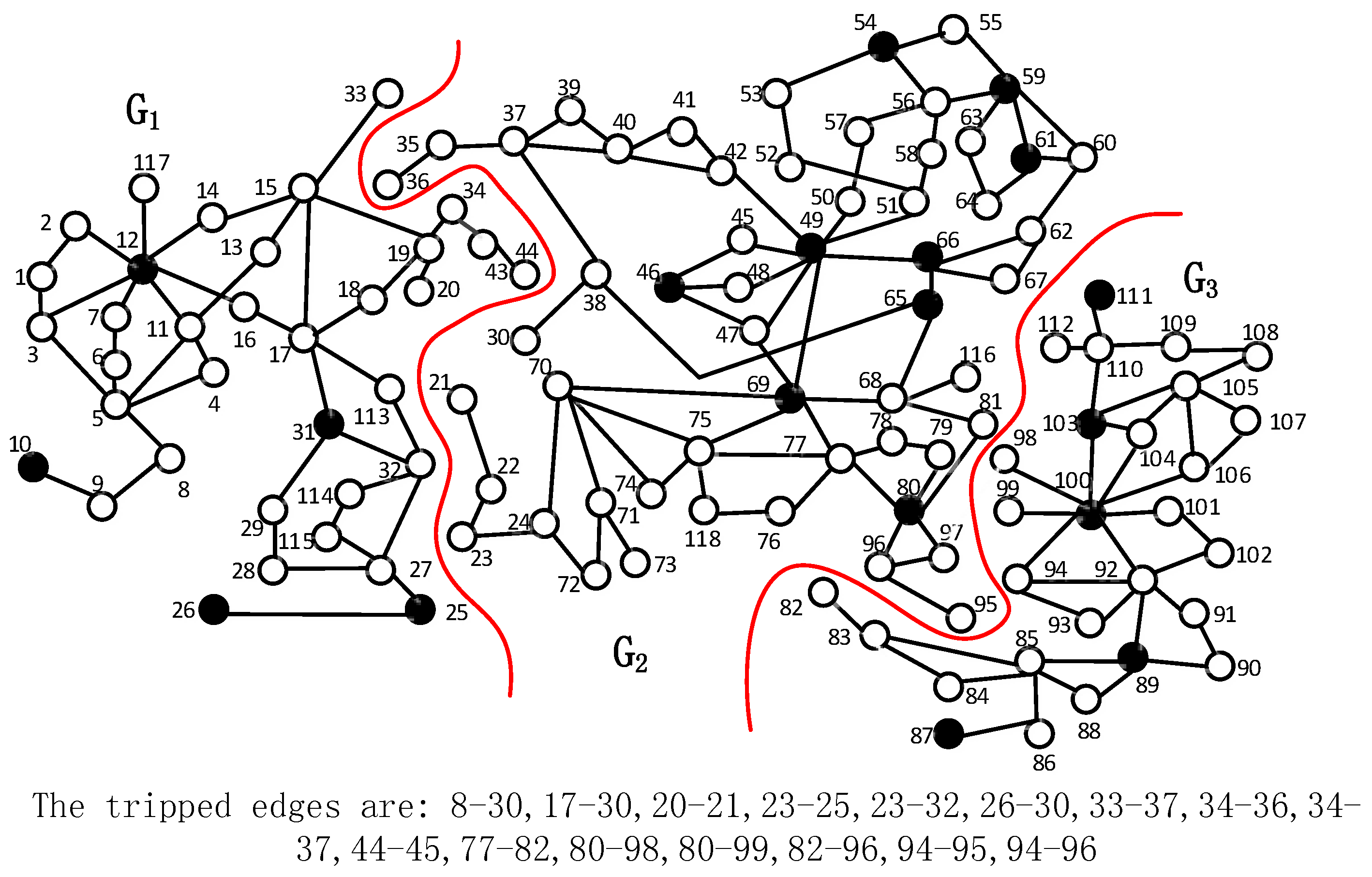
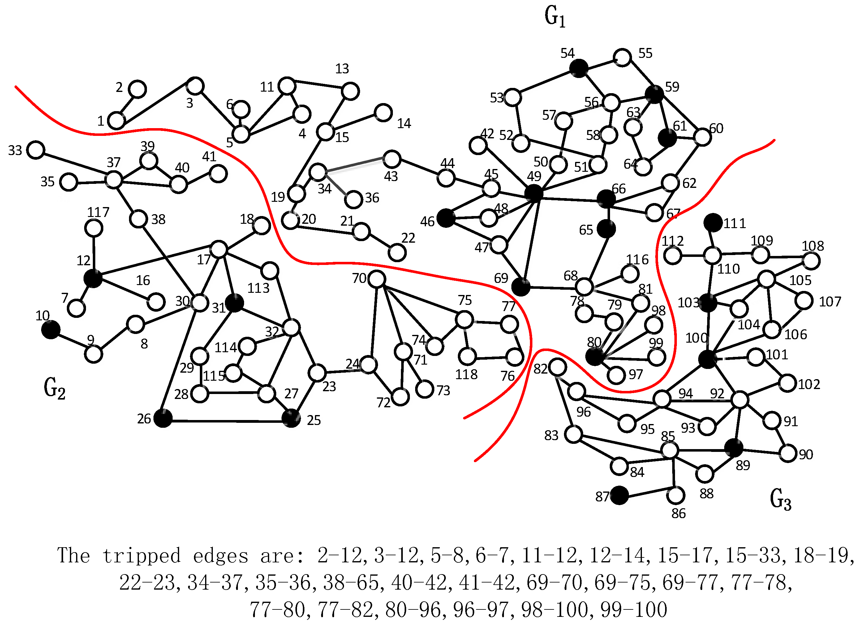
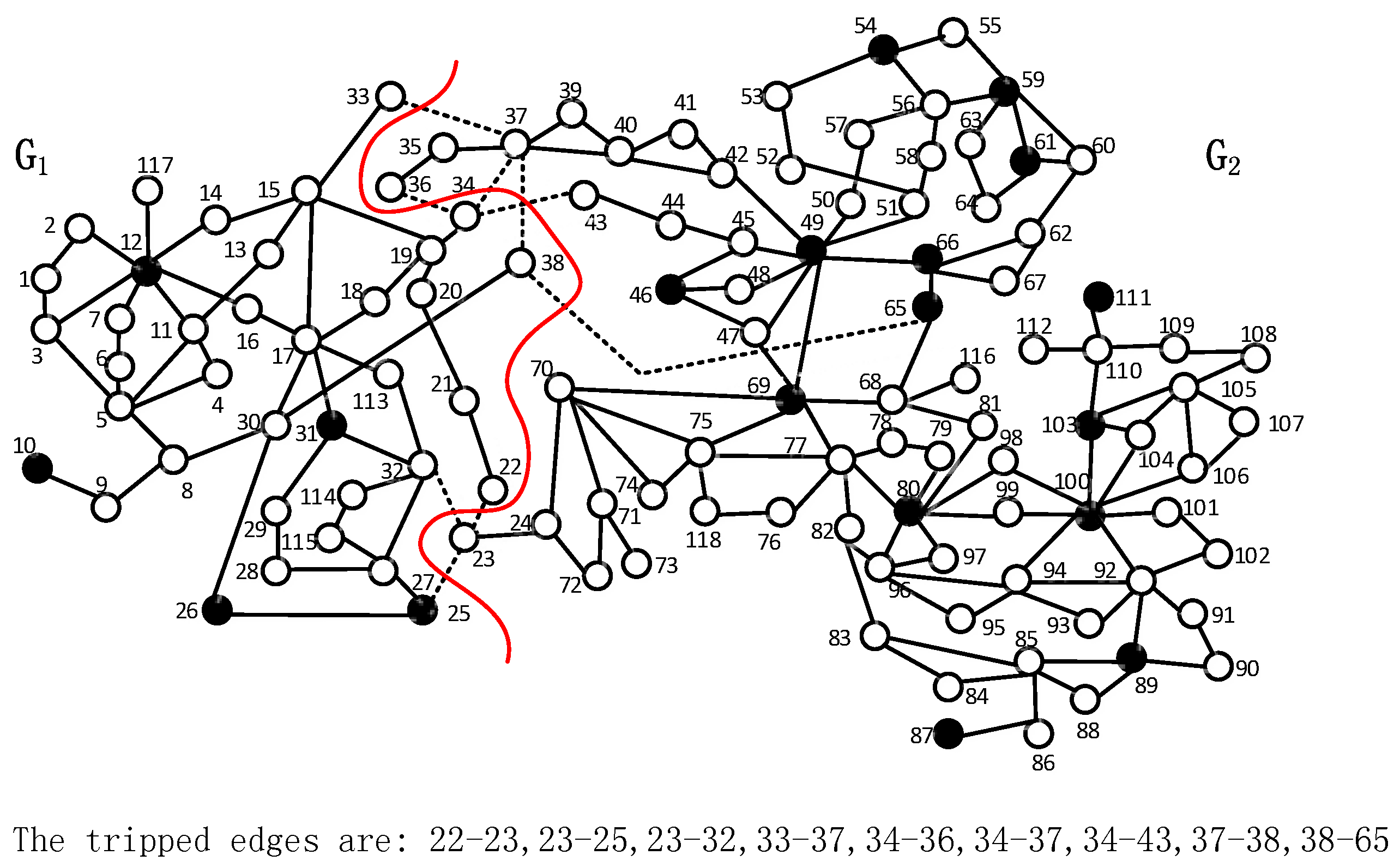
| Tabu search | 15-33, 34-36, 37-34, 34-43, 30-38, 70-24, 24-72, 111-109, 103-105, 103-104, 103-100 | 119.3 | 2.73% | 0.004 s | |
| Fast search [26] | 15-33, 34-36, 37-34, 34-43, 30-38, 70-24, 24-72, 111-109, 103-105, 103-104, 103-100 | 119.3 | 2.73% | 0.012 s | |
| OBDD-based method [18] | Run 1 | 23-24, 30-38, 19-34, 15-33, 77-82, 96-97, 80-96, 98-100, 80-99 | 148.7 | 3.40% | 5 s |
| Run 2 | 23-24, 30-38, 19-34, 33-37, 77-82, 80-97, 80-96, 98-100, 80-99 | 113.3 | 2.59% | 5 s | |
| Run 3 | 30-38, 15-33, 19-34, 69-70, 70-74, 70-75, 77-82, 96-97, 80-96, 98-100, 99-100 | 52.47 | 1.20% | 5 s | |
| Run 4 | 30-38, 15-33, 19-34, 24-70, 24-72, 77-82, 80-97, 80-96, 98-100, 99-100 | 112.6 | 2.57% | 5 s | |
| Run 5 | 77-82, 96-97, 80-96, 98-100, 80-99, 23-24, 30-38, 19-34, 33-37 | 102.7 | 2.35% | 5 s | |
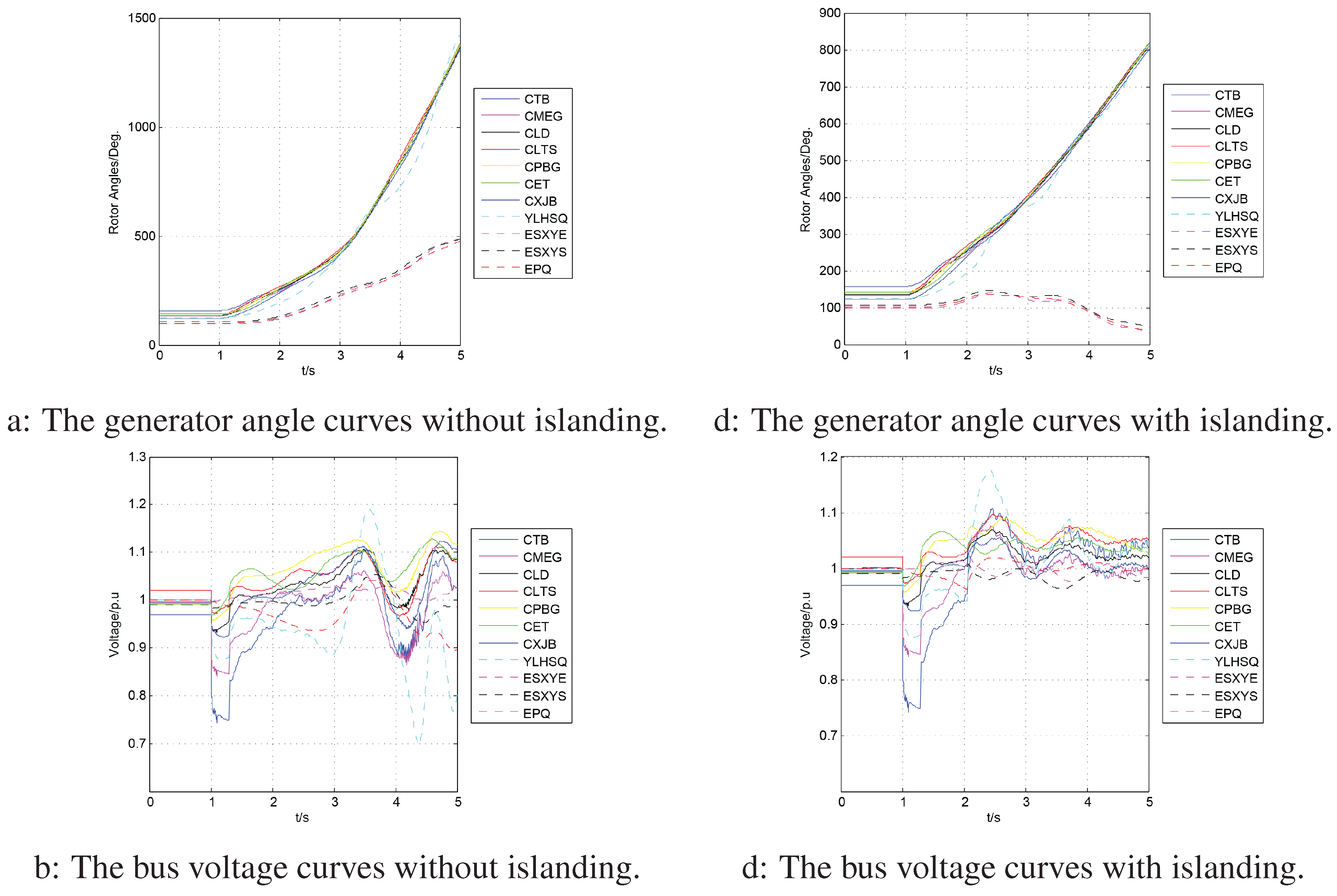
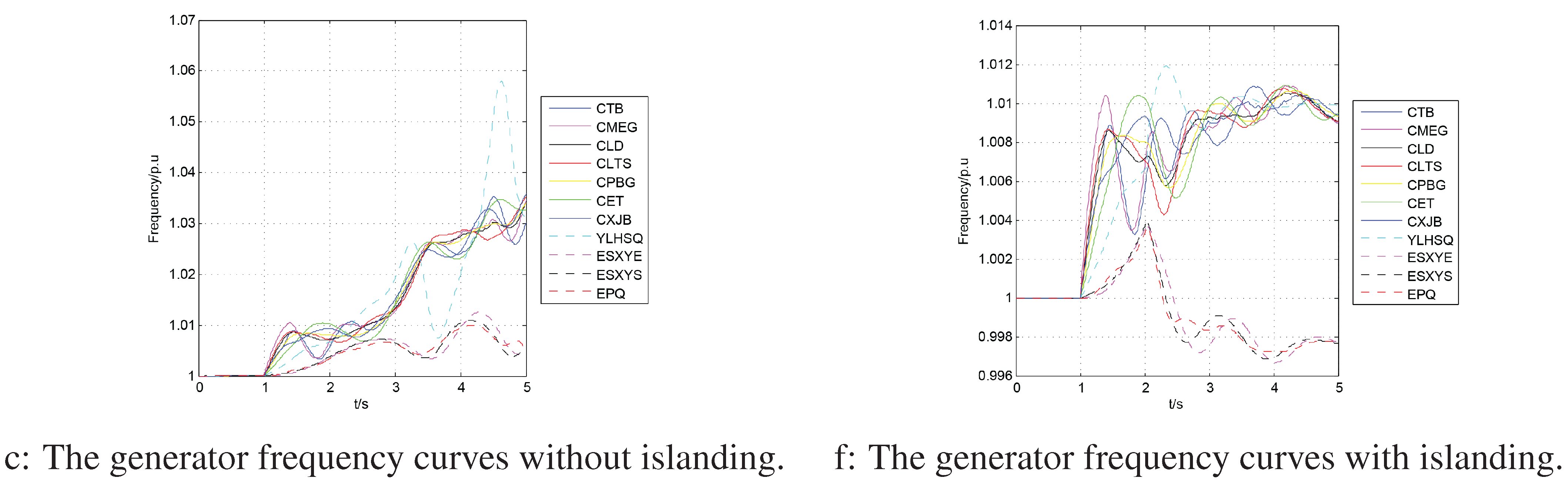
5.3. Simulation Studies
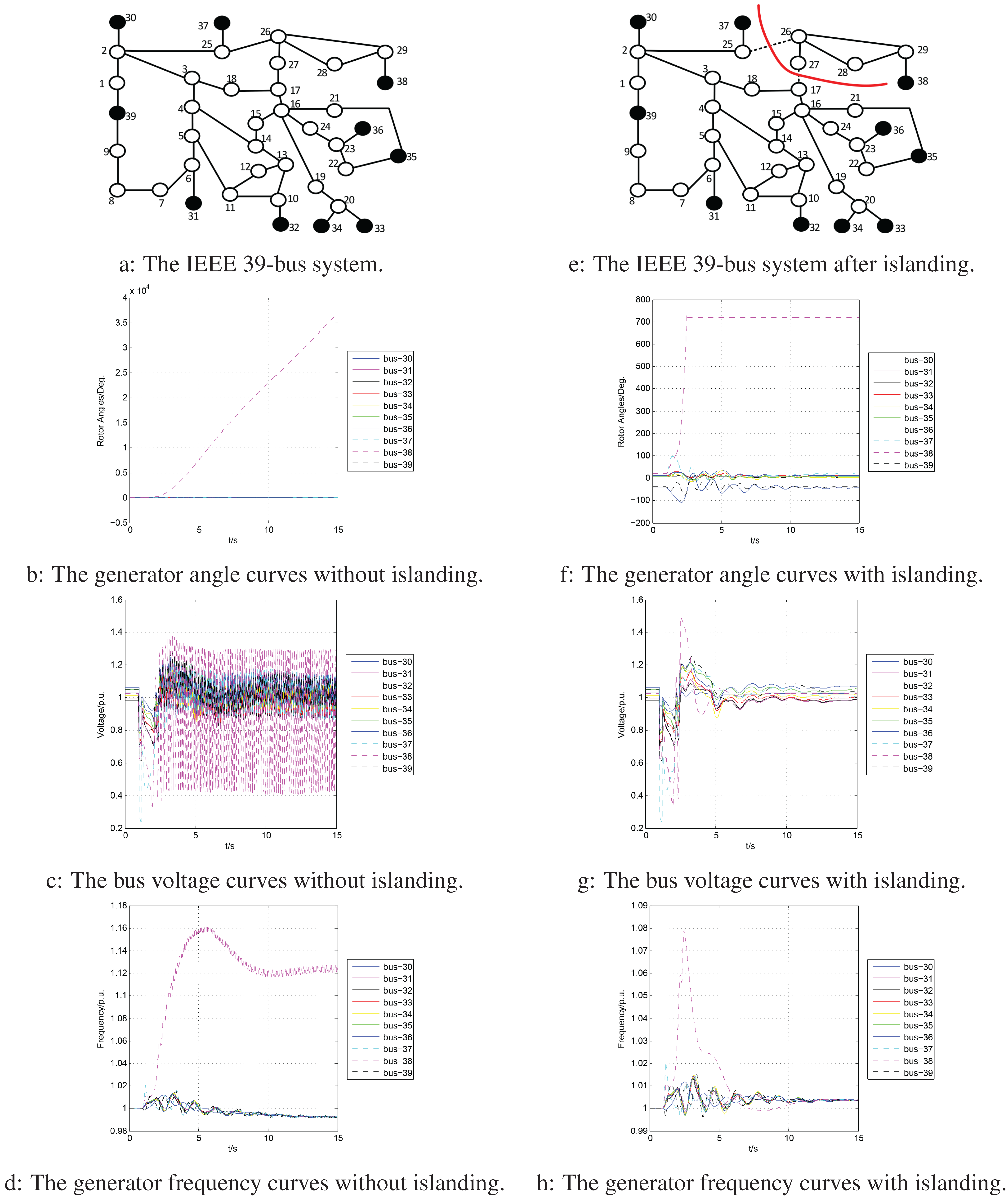
5.3.1. Test Case 1: The IEEE 39-Bus System

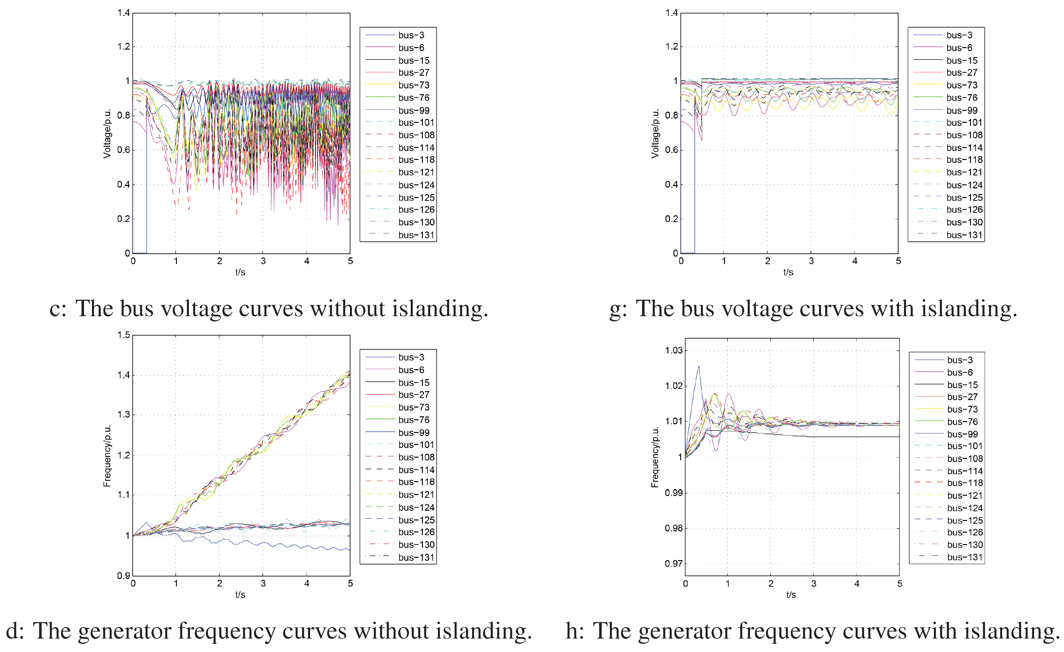
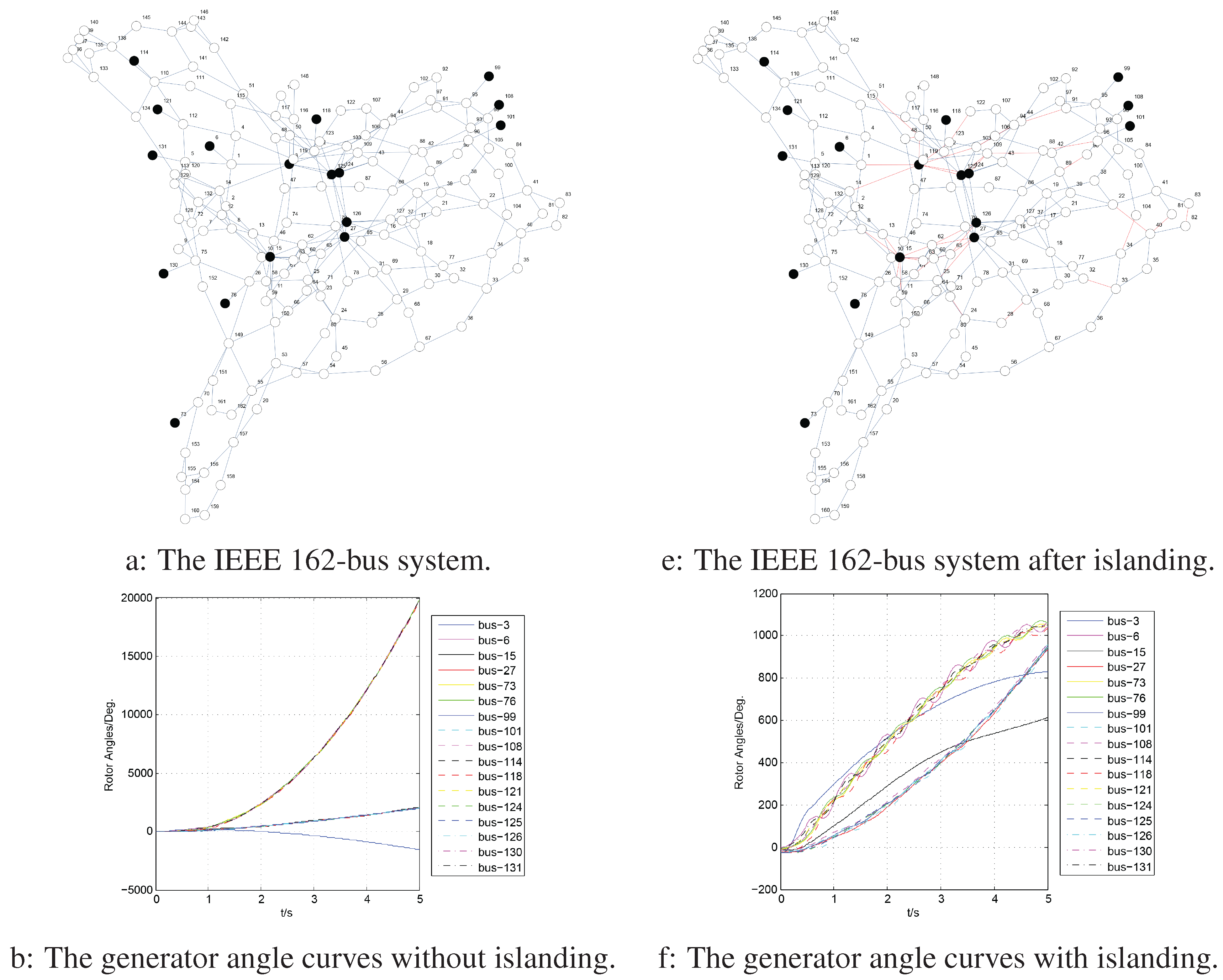
5.3.2. Test Case 2: The IEEE 162-Bus System

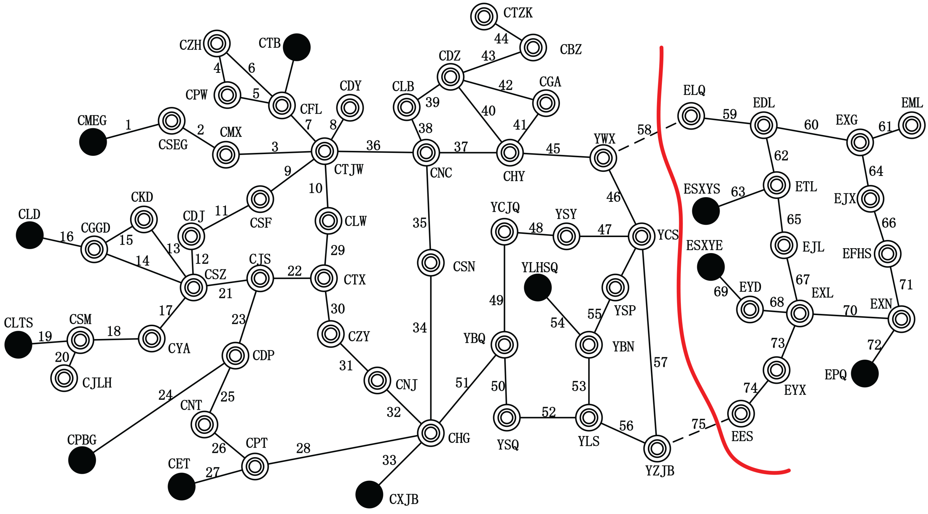
5.3.3. Test Case 3: A Reduced Power Grid of Central China
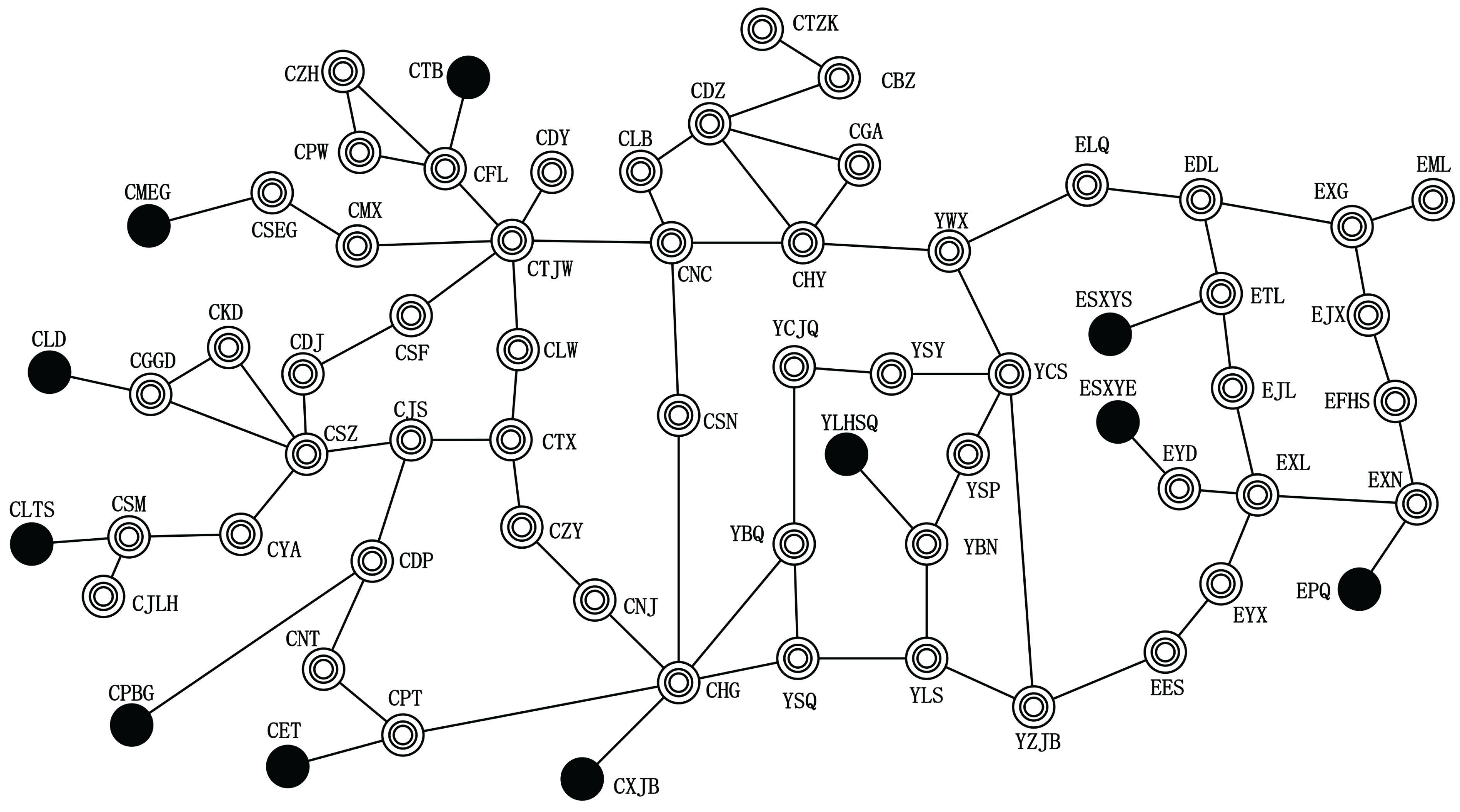


| Minimum Imbalance Power | Tripped Lines | Generation Reduction | Load Shedding |
|---|---|---|---|
| 27 MW | 58 (YWX-ELQ), 75 (YZJB-EES) | CTB (9 MW), CMEG (7 MW), CLTS (11 MW) | EXG (15 MW), ELQ (3 MW), EML (9 MW) |
6. Conclusions
Acknowledgments
Author Contributions
Conflicts of Interest
References
- Yamashita, K.; Joo, S.K.; Li, J.; Zhang, P.; Liu, C.C. Analysis, control, and economic impact assessment of major blackout events. Eur. Trans. Electr. Power 2008, 18, 854–871. [Google Scholar] [CrossRef]
- Final Report on the August 14, 2003 Blackout in the United States and Canada: Causes and Recommendations. CERTS (Consortium for Electric Reliability Technology Solutions): North America, 2004.
- Final Report of the Investigation Committee on the 28 September 2003 Blackout in Italy. UCTE (Union for the Coordination of Electricity Transmission): Europe, 2004.
- Final Report—System Disturbance on 4 November 2006. UCTE (Union for the Coordination of Electricity Transmission): Europe, 2007.
- Adibi, M.M.; Kafka, R.J.; Maram, S.; Mili, L.M. On Power System Controlled Separation. IEEE Trans. Power Syst. 2006, 21, 1894–1902. [Google Scholar] [CrossRef]
- Liu, L.; Liu, W.; Cartes, D.A.; Chung, I.Y. Slow coherency and angle modulated particle swarm optimization based islanding of large-scale power systems. Adv. Eng. Inform. 2009, 23, 45–56. [Google Scholar] [CrossRef]
- Zhao, Q.; Sun, K.; Da-Zhong, Z.; Lu, Q. A study of system splitting strategies for island operation of power system: A two-phase method based on OBDDs. IEEE Trans. Power Syst. 2003, 18, 1556–1565. [Google Scholar] [CrossRef]
- Sun, K.; Da-Zhong, Z.; Lu, Q. Splitting strategies for islanding operation of large-scale power systems using OBDD-based methods. IEEE Trans. Power Syst. 2003, 18, 912–923. [Google Scholar]
- Sun, K.; Hur, K.; Zhang, P. A new unified scheme for controlled power system separation using synchronized phasor measurements. IEEE Trans. Power Syst. 2011, 26, 1544–1554. [Google Scholar] [CrossRef]
- You, H.; Vittal, V.; Wang, X. Slow coherency-based islanding. IEEE Trans. Power Syst. 2004, 19, 483–491. [Google Scholar] [CrossRef]
- Xu, G.; Vittal, V. Slow coherency based cutset determination algorithm for large power systems. IEEE Trans. Power Syst. 2010, 25, 877–884. [Google Scholar] [CrossRef]
- Ding, L.; Gonzalez-Longatt, F.M.; Wall, P.; Terzija, V. Two-step spectral clustering controlled islanding algorithm. IEEE Trans. Power Syst. 2013, 28, 75–84. [Google Scholar] [CrossRef]
- Glover, F.; Laguna, M. Tabu Search. In Handbook of Combinatorial Optimization; Du, D.Z., Pardalos, P.M., Eds.; Springer-Verlag: Berlin, Germany, 1999; pp. 2093–2229. [Google Scholar]
- Andreev, K.; Räcke, H. Balanced graph partitioning. Theory Comput. Syst. 2006, 39, 929–939. [Google Scholar]
- Alpert, C.J.; Kahng, A.B. Recent directions in netlist partitioning: A survey. VLSI J. Integr. 1995, 19, 1–81. [Google Scholar] [CrossRef]
- Hendrickson, B.; Kolda, T.G. Graph partitioning models for parallel computing. Parallel Comput. 2000, 26, 1519–1534. [Google Scholar] [CrossRef]
- Bryant, R.E. Graph-based algorithms for Boolean function manipulation. IEEE Trans. Comput. 1986, 100, 677–691. [Google Scholar] [CrossRef]
- Sun, K.; Zheng, D.Z.; Lu, Q. A simulation study of OBDD-based proper splitting strategies for power systems under consideration of transient stability. IEEE Trans. Power Syst. 2005, 20, 389–399. [Google Scholar] [CrossRef]
- Yang, B.; Vittal, V.; Heydt, G.T. Slow-Coherency-Based Controlled Islanding; A Demonstration of the Approach on the August 14, 2003 Blackout Scenario. IEEE Trans. Power Syst. 2006, 21, 1840–1847. [Google Scholar] [CrossRef]
- Yang, B.; Vittal, V.; Heydt, G.T.; Sen, A. A Novel Slow Coherency Based Graph Theoretic Islanding Strategy. In Proceedings of the The 2007 IEEE Power Engineering Society General Meeting, Tampa, FL, USA, 24–28 June 2007; pp. 1–7.
- Trodden, P.A.; Bukhsh, W.A.; Grothey, A.; McKinnon, K.I.M. Optimization-based islanding of power networks using piecewise linear AC power flow. IEEE Trans. Power Syst. 2014, 29, 1212–1220. [Google Scholar] [CrossRef]
- Chow, J.H. Time-Scale Modeling of Dynamic Networks with Applications to Power Systems; Springer-Verlag: Berlin, Germany, 1982. [Google Scholar]
- Pampara, G.; Franken, N.; Engelbrecht, A.P. Combining Particle Swarm Optimisation with Angle Modulation to Solve Binary Problems. In Proceedings of the 2005 IEEE Congress on Evolutionary Computation, Edinburgh, Scotland, 5 September 2005; pp. 89–96.
- Sen, A.; Ghosh, P.; Vittal, V.; Yang, B. A new min-cut problem with application to electric power network partitioning. Eur. Trans. Electr. Power 2009, 19, 778–797. [Google Scholar] [CrossRef]
- Klein, P.; Ravi, R. A Nearly Best-Possible Approximation Algorithm for Node-Weighted Steiner Trees. J. Algorithms 1995, 19, 104–115. [Google Scholar] [CrossRef]
- Wang, C.G.; Zhang, B.H.; Hao, Z.G.; Shu, J.; Li, P.; Bo, Z.Q. A novel real-time searching method for power system splitting boundary. IEEE Trans. Power Syst. 2010, 25, 1902–1909. [Google Scholar] [CrossRef]
- Ding, L.; Wall, P.; Terzija, V. Constrained spectral clustering based controlled islanding. Int. J. Electr. Power Energy Syst. 2014, 63, 687–694. [Google Scholar] [CrossRef]
- Glover, F.; Laguna, M. Tabu Search*. In Handbook of Combinatorial Optimization; Pardalos, P.M., Du, D.Z., Graham, R.L., Eds.; Springer-Verlag: Berlin, Germany, 2013; pp. 3261–3362. [Google Scholar]
- Rolland, E.; Pirkul, H.; Glover, F. Tabu search for graph partitioning. Ann. Oper. Res. 1996, 63, 209–232. [Google Scholar] [CrossRef]
- Battiti, R.; Bertossi, A.A. Greedy, prohibition, and reactive heuristics for graph partitioning. IEEE Trans. Comput. 1999, 48, 361–385. [Google Scholar] [CrossRef]
- Benlic, U.; Hao, J.K. An effective multilevel tabu search approach for balanced graph partitioning. Comput. Oper. Res. 2011, 38, 1066–1075. [Google Scholar] [CrossRef] [Green Version]
- Ding, L.; Terzija, V. A New Controlled Islanding Algorithm Based on Spectral Clustering. In Proceedings of the 4th International Conference on Electric Utility Deregulation and Restructuring and Power Technologies (DRPT), Weihai, China, 6–9 July 2011; pp. 337–342.
- Molzahn, D.K.; Holzer, J.T.; Lesieutre, B.C.; DeMarco, C.L. Implementation of a large-scale optimal power flow solver based on semidefinite programming. IEEE Trans. Power Syst. 2013, 28, 3987–3998. [Google Scholar] [CrossRef]
- Qin Hu’s Web Page. Available online: https://sites.google.com/a/tigerqin.com/www/publicatoins/psip (accessed on 12 October 2015).
- Aghamohammadi, M.R.; Shahmohammadi, A. Intentional islanding using a new algorithm based on ant search mechanism. Int. J. Electr. Power Energy Syst. 2012, 35, 138–147. [Google Scholar] [CrossRef]
- Athay, T.; Podmore, R.; Virmani, S. A practical method for the direct analysis of transient stability. IEEE Trans. Power Appar. Syst. 1979, 2, 573–584. [Google Scholar] [CrossRef]
- Power System Analysis and Engineering–DIgSILENT Germany. Available online: http://www.digsilent.de/ (accessed on 12 October 2015).
- Machowski, J.; Bialek, J.; Bumby, D.J. Power System Dynamics: Stability and Control, 2nd ed.; John Wiley & Sons, Ltd: Hoboken, NJ, USA, 2008. [Google Scholar]
- Song, Y.; Ma, S.; Wu, L.; Wang, Q.; Hailei, H. PMU Placement Based on Power System Characteristics. In Proceedings of the International Conference on Sustainable Power Generation and Supply, Nanjing, China, 6–7 April 2009; pp. 1–6.
© 2015 by the authors; licensee MDPI, Basel, Switzerland. This article is an open access article distributed under the terms and conditions of the Creative Commons Attribution license (http://creativecommons.org/licenses/by/4.0/).
Share and Cite
Tang, F.; Zhou, H.; Wu, Q.; Qin, H.; Jia, J.; Guo, K. A Tabu Search Algorithm for the Power System Islanding Problem. Energies 2015, 8, 11315-11341. https://doi.org/10.3390/en81011315
Tang F, Zhou H, Wu Q, Qin H, Jia J, Guo K. A Tabu Search Algorithm for the Power System Islanding Problem. Energies. 2015; 8(10):11315-11341. https://doi.org/10.3390/en81011315
Chicago/Turabian StyleTang, Fei, Huizhi Zhou, Qinghua Wu, Hu Qin, Jun Jia, and Ke Guo. 2015. "A Tabu Search Algorithm for the Power System Islanding Problem" Energies 8, no. 10: 11315-11341. https://doi.org/10.3390/en81011315