ANN-Based Prediction and Optimization of Cooling System in Hotel Rooms

Abstract

This study aimed at developing an artificial-neural-network (ANN)-based model that can calculate the required time for restoring the current indoor temperature during the setback period in accommodation buildings to the normal set-point temperature in the cooling season. By applying the calculated time in the control logic, the operation of the cooling system can be predetermined to condition the indoor temperature comfortably in a more energy-efficient manner. Three major steps employing the numerical computer simulation method were conducted for developing an ANN model and testing its prediction performance. In the development process, the initial ANN model was determined to have input neurons that had a significant statistical relationship with the output neuron. In addition, the structure of the ANN model and learning methods were optimized through the parametrical analysis of the prediction performance. Finally, through the performance tests in terms of prediction accuracy, the optimized ANN model presented a lower mean biased error (MBE) rate between the simulation and prediction results under generally accepted levels. Thus, the developed ANN model was proven to have the potential to be applied to thermal control logic.

1. Introduction

The principal purpose of enclosed spaces such as buildings is to supply a comfortable and healthy environment to the occupants. Indoor environmental quality (IEQ) is deeply related to the realization of this purpose, and thermal quality (TQ) is a key to the creation of a proper IEQ.

In a thermally comfortable environment, the occupants’ attentiveness tends to increase, with fewer errors, resulting in advanced productivity and in the improved quality of products and services. In addition, lower rates of absenteeism and accidents, and reduced health hazards such as respiratory illness are possible [1]. The increase of the positive aspects and the reduction of the negative aspects can be ensured by properly operated thermal control systems such as heating, cooling, humidifying, and dehumidifying systems.

Besides providing a comfortable thermal environment, proper system controls can also improve the building energy efficiency. System operation at the right time and place can effectively reduce the energy consumption for thermal conditioning. Since recently, energy efficiency has also been deeply related to environmental impact. With the reduction of the energy consumption for building thermal systems, CO₂ generation, which significantly impacts global warming and ozone depletion, can also be effectively reduced [1].

Accommodation buildings such as hotels, in which thermal comfort and energy efficiency also need to be prudently managed, show specific features. First, the indoor space (e.g., rooms) is normally vacant during the day and occupied at night. Thus, thermal comfort is an important factor at night, when the occupants go back to the room.

Second, energy efficiency is not a concern of the occupants. The occupants pay the designated lodging charge, without any extra payment for thermal conditioning (heating and cooling). They may operate the heating and cooling systems excessively, beyond the actually required amounts. For example, hotel users generally do not recognize the necessity of the setback application of the heating and cooling systems.

For the proper operation of the thermal control systems in accommodation buildings, an active management process is required. The expert system needs to consider the application of the optimal set-point and setback temperatures for the system for the provision of a thermally comfortable indoor environment and for supporting improved building energy efficiency. In addition, the predetermined system operation during the setback period is necessary to restore the indoor thermal condition until the occupancy period begins. As the thermal control systems operate in a predictive manner, the occupants will feel comfortable when they go back to the room.

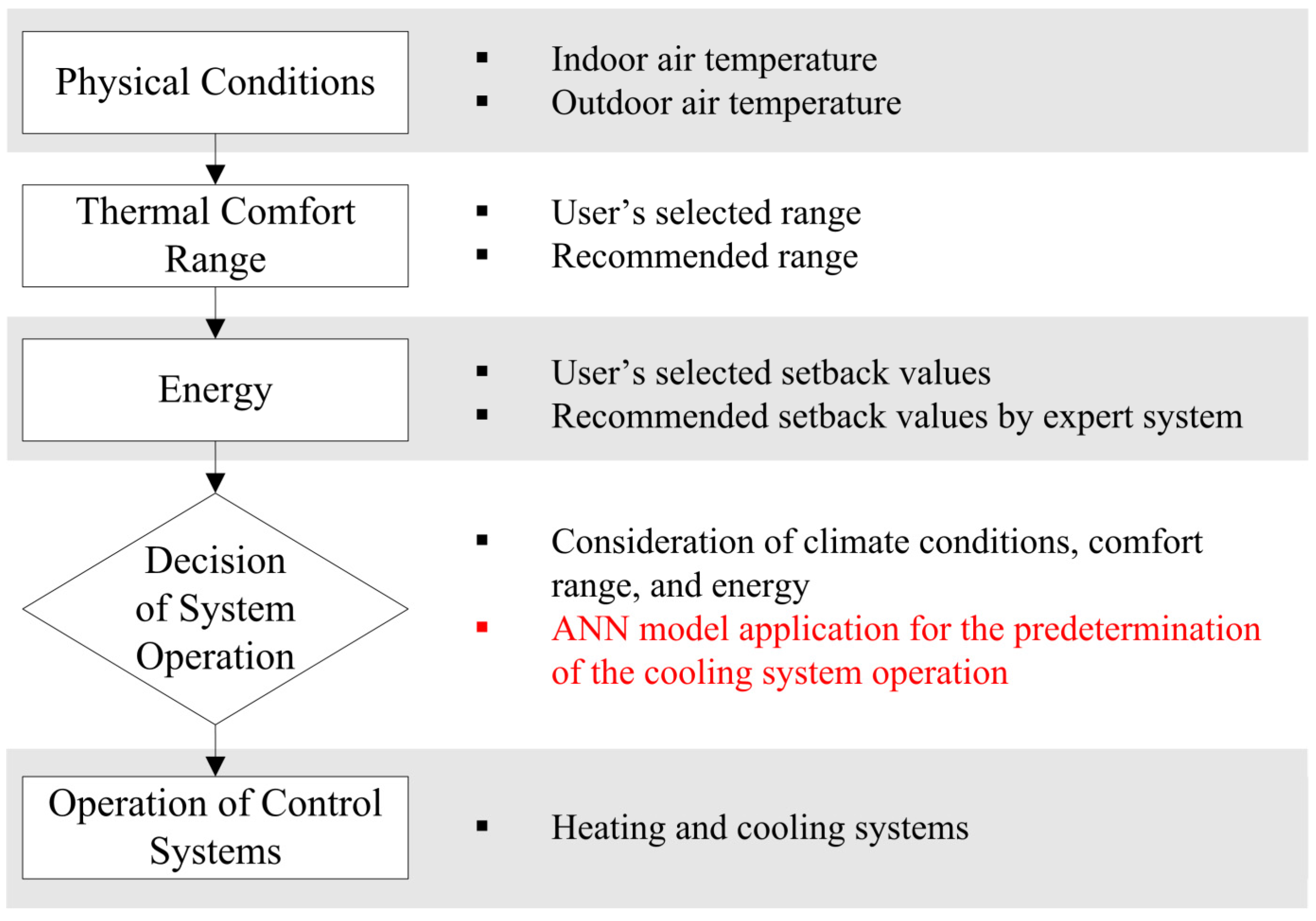
Moon and Kim proposed a logic framework (Figure 1) that deals with thermal comfort and energy efficiency synthetically, for the indoor thermal controls [2]. The logic framework consists of five steps. In the first step, which concerns the physical conditions, climatic conditions such as the indoor and outdoor air temperatures are sensed and transferred to the control panel. In the second step, the thermal comfort range that yields the operation of the heating and cooling systems is determined by either the users or logic. Similar to the second step, in the third step (concerning energy), either the users or logic set a setback value and period for reducing the energy consumption. In the fourth step (concerning the decision of system operation), the operation of the thermal control systems is determined using the information acquired in the previous steps (i.e., physical conditions, thermal comfort range, and energy). Finally, in the fifth step (concerning the operation of the control systems), the thermal control systems work to create a comfortable and energy-efficient thermal environment following the output signals decided in the previous control step.

Figure 1. A logic framework for the indoor thermal controls.

Figure 1. A logic framework for the indoor thermal controls.

With consideration of the logic framework, the purpose of this study is to develop an artificial-neural-network (ANN)-based model that can calculate the time required for restoring the current indoor temperature to the set-point temperature (TIMP_SPT) in the cooling season. The proposed model can be applied in the fourth step in Figure 1.

By applying the calculated time during the setback period, the operation of the cooling system can be predetermined to condition the indoor temperature comfortably when the normal set-point period begins. In addition, the optimal starting moment of the cooling system can be determined, and thus, the energy-inefficient earlier operation before the optimal moment can be prevented. Thus, the thermally comfortable indoor environment with improved energy efficiency is expected to be provided to accommodation buildings.

2. Development of an ANN-Based Prediction Model

The artificial-neural-network (ANN), which was created by Warren McCulloch and Walter Pitts [3], is a computational model that applies the biological processes in the human brain to artificial intelligence (AI). ANN is in mimicry of the human neural system and its learning process employing two major processes. The first of these is the feed-forward process for calculating the output from a series of inputs based on the connectivity between the neurons and the transfer functions. Through this process, outputs are produced from the model. The second process is the back-propagation process, which conducts self-learning using the difference between the desired output and the actual output for modifying connectivity [1].

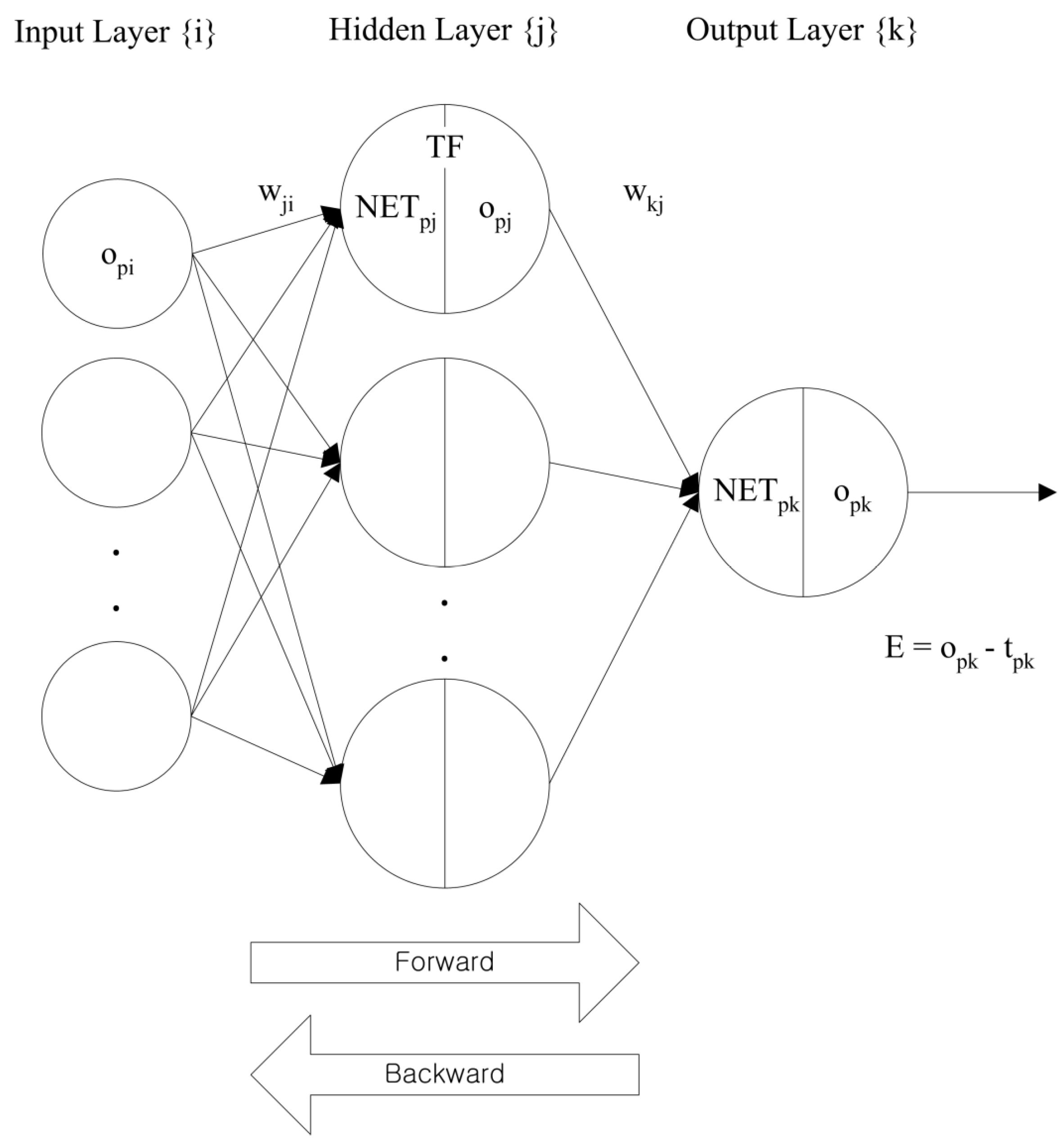
The Figure 2 shows the general structure of the ANN model. An ANN model, which employed multilayer perceptrons, is basically composed of three layers—input, hidden, and output layers. The input layer has neurons for obtaining a number of inputs. Each input value is multiplied by its own weight to be summed by the neurons in the hidden layer. The number of hidden layers and its neurons can be adjusted by the purpose of systems. Neurons in the hidden layer produce new values using a transfer function, and these new values are multiplied again by weights to output layers. Similar to the hidden layer neurons, output layer neurons also sum the values and make output, at this time, also using their transfer function.

Figure 2. A basic structure and processes of an artificial-neural-network (ANN) model.

Figure 2. A basic structure and processes of an artificial-neural-network (ANN) model.

ANN works based on the following six major components, which can be commonly applied to the neurons in input, output, or hidden layers [1]. The first component is the weighting factors (connection weight, w). Neurons obtain many inputs simultaneously. Each input has its own weights with which the impact of input can be determined so that some input is regarded as more important than others. Weights are adaptive coefficients that can be modified by training sets and learning process.

The second component is the summation function (NET). There are various summation functions for manipulating and combining inputs such as minimum, maximum, majority, product, or several normalizing methods. The most simple and common summation method is to compute the weighted sum of all of the inputs. Inputs (i₁, i₂, …, i_n) are multiplied by weights (w₁, w₂, …, w_n), then added up as weighted sum (i₁×w₁ + i₂×w₂+ … + i_n×w_n). This summed value is fed to the transfer function.

The third component is the transfer function (TF). The summation result (e.g., the weighted sum) is used in the transfer function for generating the output signal of each neuron (o_pj, o_pk). It has a threshold by which the summation result is determined. For example, when the sum is greater than the threshold, a neuron generates a signal. Or, it does not. Various transfer functions are used depending on the objectives, and the most general TF is the sigmoid function that has output ranges between 0 and 1.

The fourth component is the output function. With the exception of some network topologies, output (o) from many inputs is generally identical to the result of transfer function of the output neuron.

The fifth component is the error function and back-propagated value. The current error is the difference between the current output (o_pk) and the desired output (t_pk). This value is back propagated to a previous layer, and is used by learning function for changing weights before next cycle.

The sixth component is the learning function. A closer output to a desired output can be obtained after a learning process that is based on the learning function using error and back propagation. It is possible through the change of synaptic weights of each input.

Through these two processes of feed-forward and back-propagation, predictive and adaptive controls of the systems are feasible. For example, the future thermal conditions in the building predicted using the ANN model can be used to provide a more comfortable thermal environment. In addition, as the newly acquired data from the building can be used for the iterative training process, the ANN model adapts itself to the actual environment in the target building for the production of more accurate and stable outputs [1].

Previous studies have proven the superiority of the ANN-based model over the existing mathematical models, such as the regression or proportional-integral-derivative (PID) models. Moreover, ANN models were also proposed for the effective controls of the more diverse thermal control systems. The relevant studies and their outcomes are summarized in Table 1.

Table 1. Relevant studies using the ANN models.

Reference Number	Author(s)	Objectives and Findings
[1,2,4]	Moon, J.W.	ANN models were developed for controlling indoor temperature, humidity, and PMV of residential buildings Models controlled the heating, cooling, humidifying, and dehumidifying systems ANN-based method created more stable and comfortable thermal conditions
[5]	Yeo, M.S.; Kim, K.W.	An ANN model was developed for predicting the optimal start moment of the heating system at the beginning period of the office hour The model successfully predicted the length of time required to ascend the indoor temperature to the normal set-point temperature
[6]	Yang, I.H.; Kim, K.W.	An ANN model was developed for predicting the optimal stop moment of the heating system at the closing period of the office hour The model successfully predicted the length of time required to descend the indoor temperature to the normal set-point temperature.
[7]	Ben-Nakhi, A.E.; Mahmoud, M.A.	An ANN model was developed for predicting the optimal end of setback time of the cooling system for the start of the business hours The model presented its prediction accuracy with strong correlation coefficient with simulated results.
[8,9]	Argiriou, A.A. et al.	An ANN model was applied for predicting the optimal heating supply of hydronic heating systems of solar buildings The proposed method significantly reduced energy consumption by 15% compared to the conventional controller.
[10]	Morel, N. et al.	Three ANN models were developed for controlling a radiant heating system in residential buildings—(1) for predicting outdoor temperature; (2) for predicting solar radiation; and (3) for predicting future indoor temperature More comfortable thermal condition was provided with improved energy-efficiency.
[11,12]	Lee, J.Y. et al.	An ANN model was developed for operating a radiant under-floor heating system Using the proposed method, heating system worked in the predetermined manner resulting in the significant reduction of overshoot and undershoot of indoor temperature.
[13]	Abbassi, A.; Bahar, L.	An ANN model was developed for operating an evaporative condenser and its performance was compared with a PID controller The ANN-based method proved to reduce the process errors compared to those of the PID controller.
[14]	Chow, T.T. et al.	Incorporative method using ANN and Genetic algorithm (GA) was proposed for the optimal use of energy (fuel and electricity) for operating an absorption chiller system ANN model proved its prediction accuracy for the mass flow rated of diesel oil, electric power of the cooling water pump, chilled water pump, and coefficient of performance (COP) of the system.
[15,16,17]	Hikmet, E. et al.	ANN-based prediction models were developed for operating ground coupled heat pump system (GCHP) They proved applicability with accurate prediction results for the coefficient of performance (COP) of ground coupled heat pump (GCHP) system.

Table 1. Relevant studies using the ANN models.

Reference Number	Author(s)	Objectives and Findings
[1,2,4]	Moon, J.W.	ANN models were developed for controlling indoor temperature, humidity, and PMV of residential buildings Models controlled the heating, cooling, humidifying, and dehumidifying systems ANN-based method created more stable and comfortable thermal conditions
[5]	Yeo, M.S.; Kim, K.W.	An ANN model was developed for predicting the optimal start moment of the heating system at the beginning period of the office hour The model successfully predicted the length of time required to ascend the indoor temperature to the normal set-point temperature
[6]	Yang, I.H.; Kim, K.W.	An ANN model was developed for predicting the optimal stop moment of the heating system at the closing period of the office hour The model successfully predicted the length of time required to descend the indoor temperature to the normal set-point temperature.
[7]	Ben-Nakhi, A.E.; Mahmoud, M.A.	An ANN model was developed for predicting the optimal end of setback time of the cooling system for the start of the business hours The model presented its prediction accuracy with strong correlation coefficient with simulated results.
[8,9]	Argiriou, A.A. et al.	An ANN model was applied for predicting the optimal heating supply of hydronic heating systems of solar buildings The proposed method significantly reduced energy consumption by 15% compared to the conventional controller.
[10]	Morel, N. et al.	Three ANN models were developed for controlling a radiant heating system in residential buildings—(1) for predicting outdoor temperature; (2) for predicting solar radiation; and (3) for predicting future indoor temperature More comfortable thermal condition was provided with improved energy-efficiency.
[11,12]	Lee, J.Y. et al.	An ANN model was developed for operating a radiant under-floor heating system Using the proposed method, heating system worked in the predetermined manner resulting in the significant reduction of overshoot and undershoot of indoor temperature.
[13]	Abbassi, A.; Bahar, L.	An ANN model was developed for operating an evaporative condenser and its performance was compared with a PID controller The ANN-based method proved to reduce the process errors compared to those of the PID controller.
[14]	Chow, T.T. et al.	Incorporative method using ANN and Genetic algorithm (GA) was proposed for the optimal use of energy (fuel and electricity) for operating an absorption chiller system ANN model proved its prediction accuracy for the mass flow rated of diesel oil, electric power of the cooling water pump, chilled water pump, and coefficient of performance (COP) of the system.
[15,16,17]	Hikmet, E. et al.	ANN-based prediction models were developed for operating ground coupled heat pump system (GCHP) They proved applicability with accurate prediction results for the coefficient of performance (COP) of ground coupled heat pump (GCHP) system.

In this study, an ANN-based prediction model was designed to calculate the amount of operating time (TIME_SPT) required for restoring the current indoor temperature under the setback condition in accommodation buildings to the normal set-point condition in the cooling season. For example, when the current indoor temperature is 28.0 °C during the setback period in summer, and the normal set-point temperature is 24.5 °C, the prediction model calculates the amount of operating time required to change the indoor temperature from 28.0 to 24.5 °C. The calculated value (TIME_SPT) will be employed in the control logic afterward to predetermine the cooling system operation.

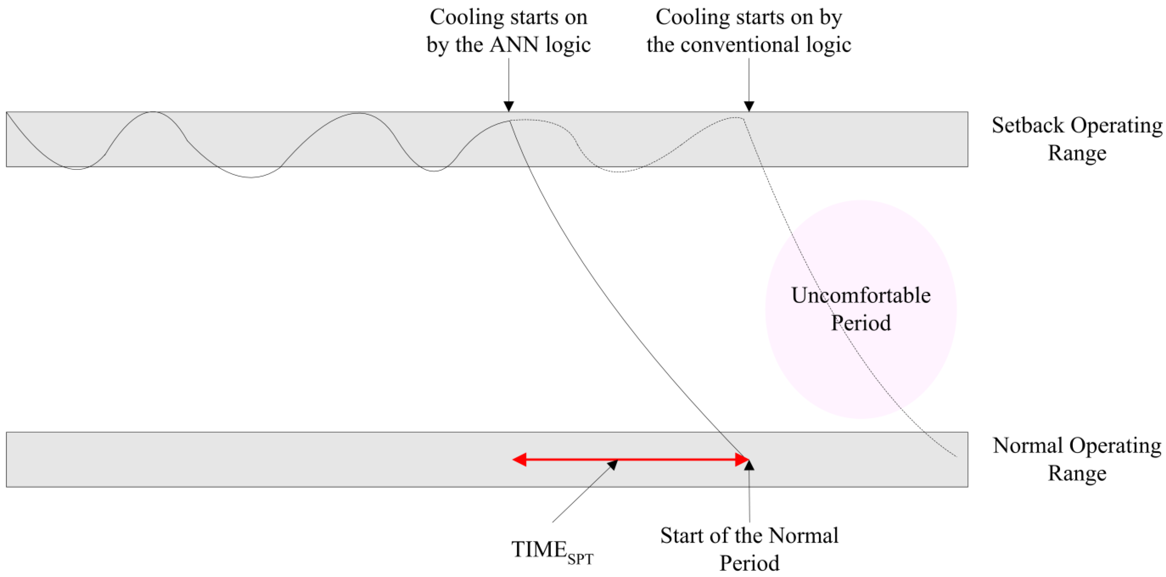
Figure 3 conceptually shows the potentials of the thermal control logic that employs the ANN-based prediction model. During the setback period, the indoor temperature is maintained within the setback operating range. At every control cycle, the prediction model will calculate the TIME_SPT. If the summation of the current time of the day and the TIME_SPT is larger than the starting moment of the normal set-point period, the cooling system begins to work even though the setback is currently applied for operating the cooling system. If the cooling device is operated in a predictive manner, the indoor temperature will return to a point near the comfortable condition when the normal set-point is applied.

Figure 3. Conceptual comparison of the normal logic and the predicted logic.

Figure 3. Conceptual comparison of the normal logic and the predicted logic.

In contrast, the conventional non-predictive logic will begin to operate the cooling system when the normal set-point is applied. A specific time is required to return the indoor temperature to the normal operating range. Such time corresponds to the uncomfortable period, which can make the occupant feel hot.

For preventing such phenomenon, the conventional approach is to turn on the cooling system at some point earlier than the moment when the normal set-point is applied. The starting moment is normally determined by the building manager or the occupants themselves, using their inaccurate past experiences. In this case, the cooling system could start working before it is actually required, resulting in energy-inefficiency.

Thus, as the predictive model is applied in the control logic, its two major advantages over the conventional logic are expected to be realized. Its first advantage is that more comfortable temperature conditions can be provided, and the second is that the unnecessary energy consumption for space cooling during the setback period can be prevented.

Compared to the previous studies which were conducted for development of the ANN models for the cooling system, this study adopted a procedurally definite process for the model development. Statistical analysis was conducted for selecting the input variables of the model and the optimal structure and the learning methods was parametrically determined after performance comparison. This procedure can present a sound basis when other ANN models are developed for building system controls.

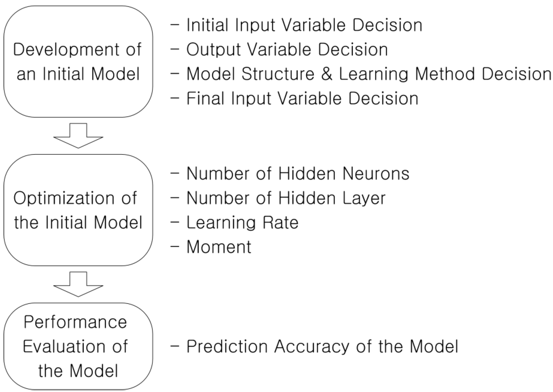
Three major steps were carried out for the proposal of an ANN-based prediction model, as shown in Figure 4. The first step was for developing an initial model, in which the initial input and output variables, the numbers of hidden neurons and layers, and the learning method of the ANN model were decided. In particular, the input variables that had statistically significant relationships with the output variable were selected as the initial variables.

Figure 4. Development process of the prediction model.

Figure 4. Development process of the prediction model.

The next step was carried out for optimizing the initial ANN model for the purpose of calculating a more accurate and stable output. In this process, the optimal numbers of hidden neurons and layers, the learning rate, and the momentum rate were determined and applied to the ANN model.

The last step was to evaluate the performance of the optimized ANN model. The prediction accuracy of the developed ANN model was validated based on the comparison of its results with the data acquired from the simulation as described in Section 2.1. The prediction accuracy would support the applicability of the prediction model to the control logic.

2.1. Initial Model Development

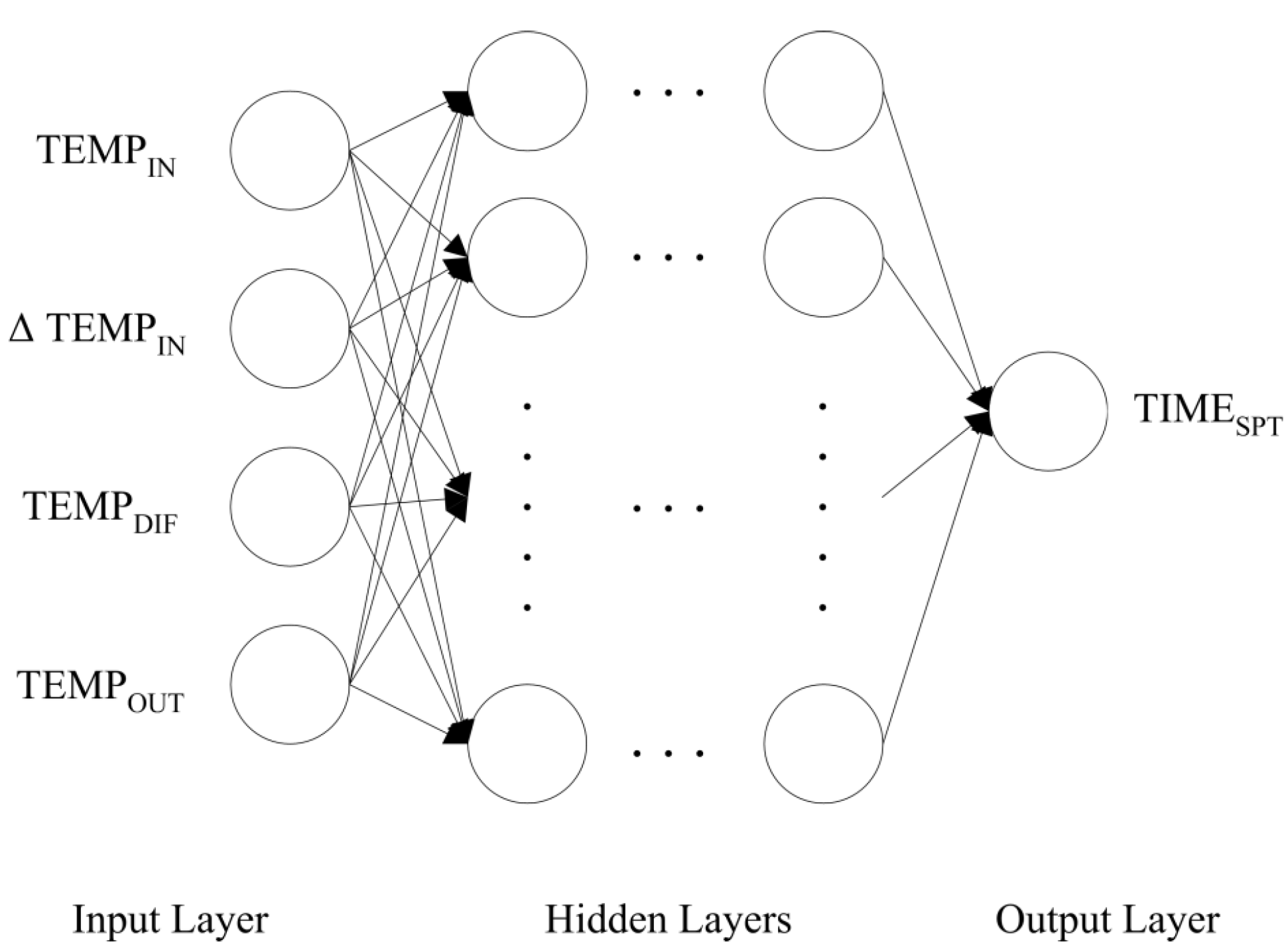
The initial structure of the ANN model is shown in Figure 5, and its composition is summarized in Table 2.

Figure 5. Structure of the initial ANN model.

Figure 5. Structure of the initial ANN model.

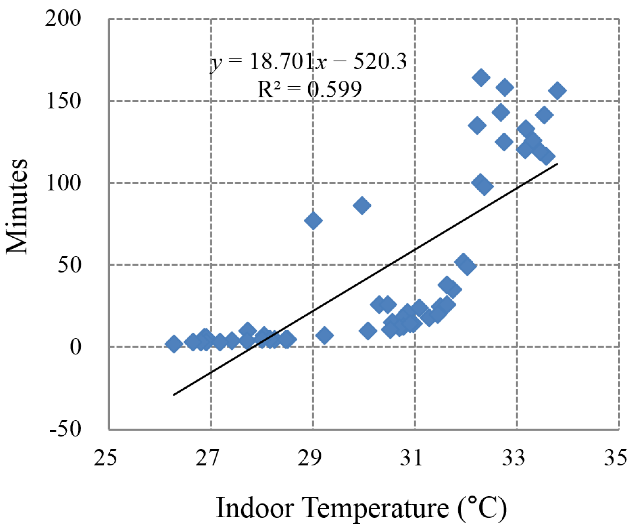
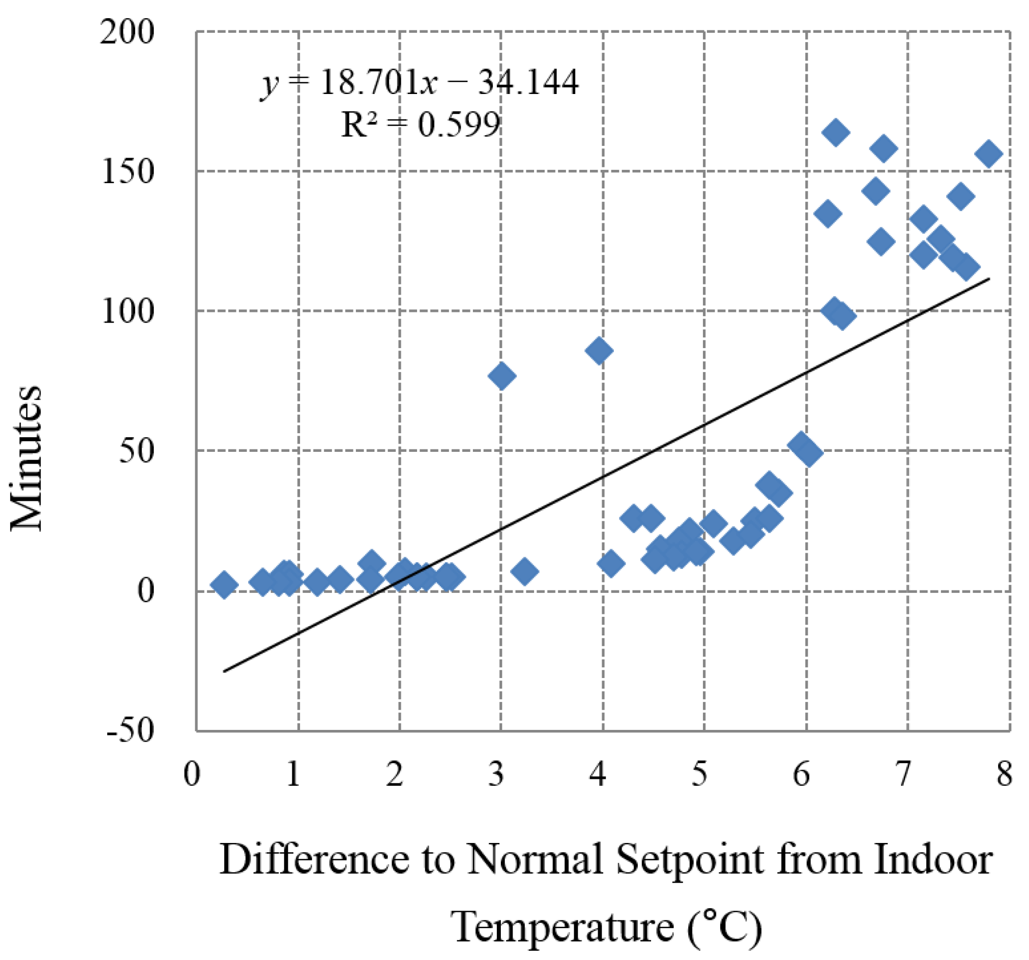
The input variables initially consisted of the indoor air temperature (TEMPIN, °C), indoor air temperature change from the preceding control cycle’s indoor air temperature (ΔTEMPIN, °C), temperature difference from the set-point temperature (TEMPDIF, °C), and outdoor air temperature (TEMPOUT, °C) for predicting the output variable, which is the predicted time required for changing from the current temperature to the set-point temperature (TIMPSPT, minutes). The input values for each neuron were normalized between 0 and 1. The normalized values were represented as 10–50, −10–10, 0–20, and −20–40 °C for TEMPIN, ΔTEMPIN, TEMPDIF, and TEMPOUT, respectively. The final input variable was determined through the statistical analysis of the relationship with the output variable.

Table 2. Initial composition of the prediction model.

Model Components		Contents
Structure	Input Layer	Number of neurons: 4 (1) TEMPIN (2) ΔTEMPIN (3) TEMPDIF (4) TEMPOUT
	Hidden Layer	Number of Layers: 1 Number of neurons: 9 using Nh = 2Ni + 1 [18,19]
	Output Layer	Number of neuron: 1 (1) TIMPSPT
Transfer Function	Hidden Neurons	Tangent Sigmoid
	Output Neurons	Pure Linear
Training Method	Goal	0.0 minute (mean square error)
	Epoch	1000 times
	Learning rate	0.6 [20]
	Momentum rate	0.4 [20]
	Algorithm	Levenberg-Marquardt [2,4]
	Number of data sets	45 using Nd = (Nh − (Ni + No)/2 )2 [21]
	Data management technique	Sliding-window method

Table 2. Initial composition of the prediction model.

Model Components		Contents
Structure	Input Layer	Number of neurons: 4 (1) TEMPIN (2) ΔTEMPIN (3) TEMPDIF (4) TEMPOUT
	Hidden Layer	Number of Layers: 1 Number of neurons: 9 using Nh = 2Ni + 1 [18,19]
	Output Layer	Number of neuron: 1 (1) TIMPSPT
Transfer Function	Hidden Neurons	Tangent Sigmoid
	Output Neurons	Pure Linear
Training Method	Goal	0.0 minute (mean square error)
	Epoch	1000 times
	Learning rate	0.6 [20]
	Momentum rate	0.4 [20]
	Algorithm	Levenberg-Marquardt [2,4]
	Number of data sets	45 using Nd = (Nh − (Ni + No)/2 )2 [21]
	Data management technique	Sliding-window method

The number of hidden layers was initially designated as one, and the number of hidden neurons as nine, using the given equation, which would be optimized in the second step of the development (see Section 2.2). The tangent-sigmoid and pure linear transfer functions were employed as the transfer functions for the hidden and output neurons, respectively. For training the ANN model, a 0.0-minute-goal, 1000-times-epoch, 0.6-learning-rate, 0.4-momentum rate, and Levenberg-Marquardt algorithm for adapting weights between neurons was applied. Since the goal was assigned to 0.0, the training would be continued until the calculated output and the desired output became identical. However, the epoch was 1000 times, thus the training would quit when the 1000 times of training process was completed. The learning rate controls the changing size of weight and bias in the process of training. In addition, the momentum rate is used for preventing the model from converging to a local minimum or saddle point. The optimal learning rate and momentum rate could also be found in the second step. In addition, 45 training datasets were prepared based on the given equation in Table 3, which considers the number of input, hidden, and output neurons for estimating proper number of training datasets. In addition, the sliding-window method was used for managing the training datasets, thus the model can reflect the iterative changing environment around buildings. The training datasets were composed of four input components and one output component, as presented in Table 3.

Table 3. Composition of the training datasets.

Data Sets		1	2	3	4	5	6	…
Input components (actual value in parenthesis, °C)	TEMPIN	0.4512 (28.05)	0.4217 (26.87)	0.4430 (27.72)	0.4227 (26.91)	0.5076 (30.31)	0.5118 (30.47)	…
	ΔTEMPIN	0.5189 (0.38)	0.4797 (-0.41)	0.5220 (0.44)	0.4853 (-0.29)	0.5113 (0.23)	0.5093 (0.19)	…
	TEMPDIF	0.1023 (2.05)	0.4337 (0.87)	0.8604 (1.72)	0.4545 (0.91)	0.2153 (4.31)	0.2236 (4.47)	…
	TEMPOUT	0.7540 (25.24)	0.7383 (24.30)	0.7118 (22.71)	0.7914 (27.48)	0.7651 (25.91)	0.7642 (25.85)	…
Output component, minutes	TIMPSPT	7	6	1	6	26	26	…

Table 3. Composition of the training datasets.

Data Sets		1	2	3	4	5	6	…
Input components (actual value in parenthesis, °C)	TEMPIN	0.4512 (28.05)	0.4217 (26.87)	0.4430 (27.72)	0.4227 (26.91)	0.5076 (30.31)	0.5118 (30.47)	…
	ΔTEMPIN	0.5189 (0.38)	0.4797 (-0.41)	0.5220 (0.44)	0.4853 (-0.29)	0.5113 (0.23)	0.5093 (0.19)	…
	TEMPDIF	0.1023 (2.05)	0.4337 (0.87)	0.8604 (1.72)	0.4545 (0.91)	0.2153 (4.31)	0.2236 (4.47)	…
	TEMPOUT	0.7540 (25.24)	0.7383 (24.30)	0.7118 (22.71)	0.7914 (27.48)	0.7651 (25.91)	0.7642 (25.85)	…
Output component, minutes	TIMPSPT	7	6	1	6	26	26	…

MATLAB (Matrix Laboratory) and its neural network [22] toolbox were used for developing the ANN model. The developed model was connected to the TRNSYS (Transient Systems Simulation) software [23] for acquiring training datasets and checking datasets for analyzing the relationship between the input variables and the output variable and for optimizing model and testing prediction performance of the optimized model.

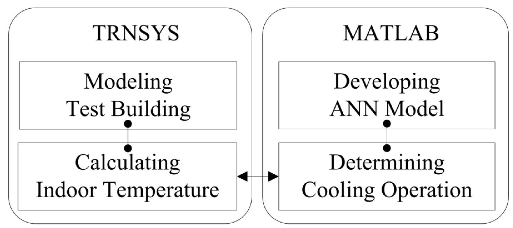
As shown in Figure 6, the TRNSYS software was employed for modeling the test building with cooling system, and calculating new indoor temperature according to the cooling system operation. On the other hand, the MATLAB software was used for developing the ANN model and for determining cooling system’s operation.

Figure 6. Incorporative process of TRNSYS and MATLAB.

Figure 6. Incorporative process of TRNSYS and MATLAB.

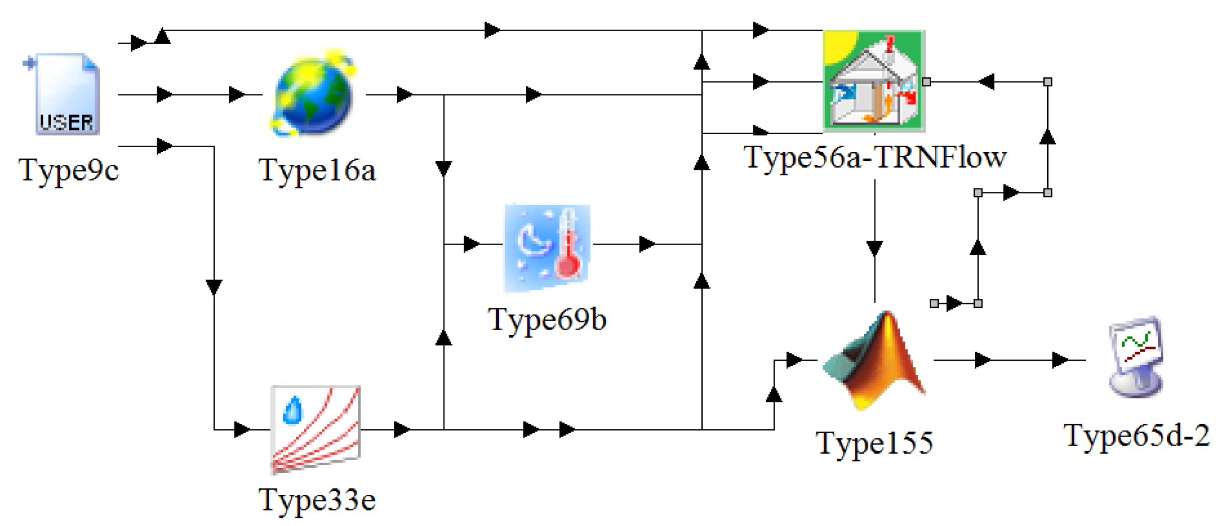
Figure 7 shows the modeling result using the MATLAB and TRNSYS in an incorporative manner. Seven types of components in TRNSYS comprised the simulation model. The roles of each type are explained in Table 4.

Figure 7. Composition of the simulation model.

Figure 7. Composition of the simulation model.

Table 4. Roles of Transient Systems Simulation (TRNSYS) types.

Types	Roles
Type 9c	Importing a TMY2 weather file for the building location Transferring required weather data to Type56a-TRNFlow, Type16a, and Type33e
Type 16a	Calculating solar radiation on the each building surface Transferring calculated data to Type56a-TRNFlow and Type69b
Type 33e	Calculating dew-point temperature of exterior Transferring calculated data to Type56a-TRNFlow, Type69b, and Type155
Type 69b	Calculating sky temperature Transferring the calculated data to Type56a-TRNFlow
Type 56a-TRNFlow	Calling TRNBUILD result (building modeling result) Calculating indoor temperature of the building Transferring the calculated data to Type 155
Type 155	Calling MATLAB and the ANN model Producing training and checking datasets Calculating operating signal for the cooling system Transferring the calculated signal to Type56a-TRNFlow
Type 65d-2	Producing the output file

Table 4. Roles of Transient Systems Simulation (TRNSYS) types.

Types	Roles
Type 9c	Importing a TMY2 weather file for the building location Transferring required weather data to Type56a-TRNFlow, Type16a, and Type33e
Type 16a	Calculating solar radiation on the each building surface Transferring calculated data to Type56a-TRNFlow and Type69b
Type 33e	Calculating dew-point temperature of exterior Transferring calculated data to Type56a-TRNFlow, Type69b, and Type155
Type 69b	Calculating sky temperature Transferring the calculated data to Type56a-TRNFlow
Type 56a-TRNFlow	Calling TRNBUILD result (building modeling result) Calculating indoor temperature of the building Transferring the calculated data to Type 155
Type 155	Calling MATLAB and the ANN model Producing training and checking datasets Calculating operating signal for the cooling system Transferring the calculated signal to Type56a-TRNFlow
Type 65d-2	Producing the output file

The datasets for training and checking the ANN model were collected from a module that was in the center of the nine identical modules. Three modules comprised one floor, thus the target module was in the center of the second floor of the three story test building. All modules faced outside to the south and north. The features of the module, such as the location, climate condition, dimension, envelope insulation, applied system, internal gain, and infiltration rate, are summarized in Table 5.

Table 5. Features of a test module.

Test Module Components		Contents
Weather Data		TMY2 for Seoul, South Korea (latitude: 37.56 N, longitude: 126.98 E)
Climate Condition of the Building Site		Cold in winter: 1.7 °C air temperature and 59.1% relative humidity from November to February on average. Hot and humid in summer: 23.5 °C air temperature and72.7% relative humidity from June to September on average
Dimension	Module	26.64 m2 3.6 m wide × 7.4 m deep × 2.7 m high
	Window	1.8 m2 2.0 m wide ×0.9 m high
Envelope Insulation [m2 K/W] [24]		Exterior walls	2.801
		Interior walls, roof, and floor	0.492
		Windows	0.353
Systems Applied [25]		Convective cooling: 8,901 kJ/hr heat removal
Internal Gain		1.occupant seated, doing light work (typing) 1 computer and printer 5 W/m2 lighting fixtures
Infiltration Rate [24]		0.7 ACH

Table 5. Features of a test module.

Test Module Components		Contents
Weather Data		TMY2 for Seoul, South Korea (latitude: 37.56 N, longitude: 126.98 E)
Climate Condition of the Building Site		Cold in winter: 1.7 °C air temperature and 59.1% relative humidity from November to February on average. Hot and humid in summer: 23.5 °C air temperature and72.7% relative humidity from June to September on average
Dimension	Module	26.64 m2 3.6 m wide × 7.4 m deep × 2.7 m high
	Window	1.8 m2 2.0 m wide ×0.9 m high
Envelope Insulation [m2 K/W] [24]		Exterior walls	2.801
		Interior walls, roof, and floor	0.492
		Windows	0.353
Systems Applied [25]		Convective cooling: 8,901 kJ/hr heat removal
Internal Gain		1.occupant seated, doing light work (typing) 1 computer and printer 5 W/m2 lighting fixtures
Infiltration Rate [24]		0.7 ACH

2.2. Initial Model Optimization

To calculate a more accurate and stable output from the prediction model, the initial ANN model was optimized using a parametrical optimization process based on the method used in the previous study [5,21]. The number of hidden neurons, number of hidden layers, learning rate, and momentum rate were sequentially optimized. When the first component (i.e., number of hidden neurons) was tested for finding the optimal number, the other components (i.e., number of hidden layers, learning rate, and moment) were fixed as the initial values.

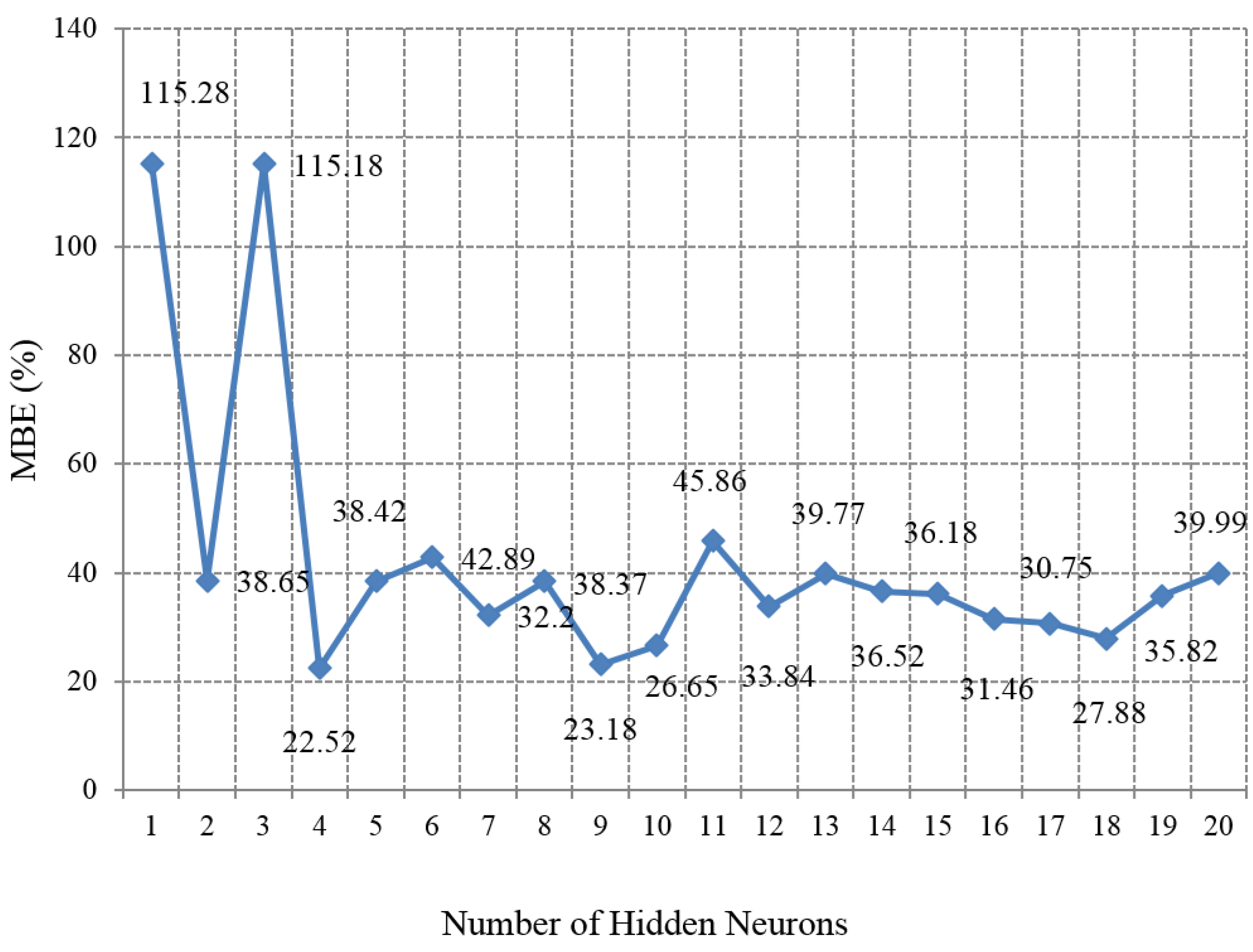
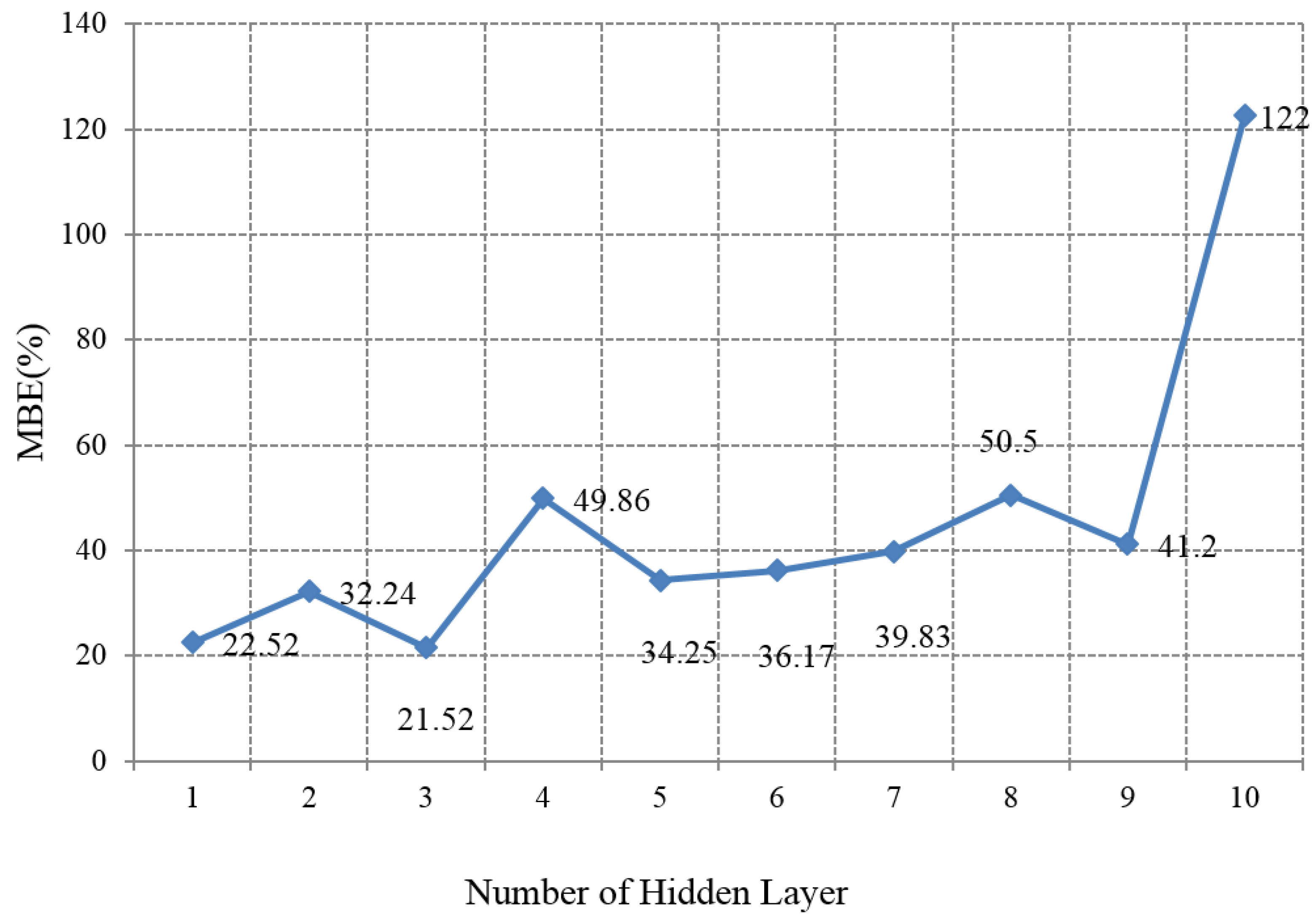
After finding the optimal value for the first component, the next component was tested. In this case, the first component was fixed as the optimal value, and the other two components were fixed as the initial values. This process was carried out until the optimal value of the last component (i.e., moment) was determined. Table 6 summarizes the parametrical values that were used for optimizing each component.

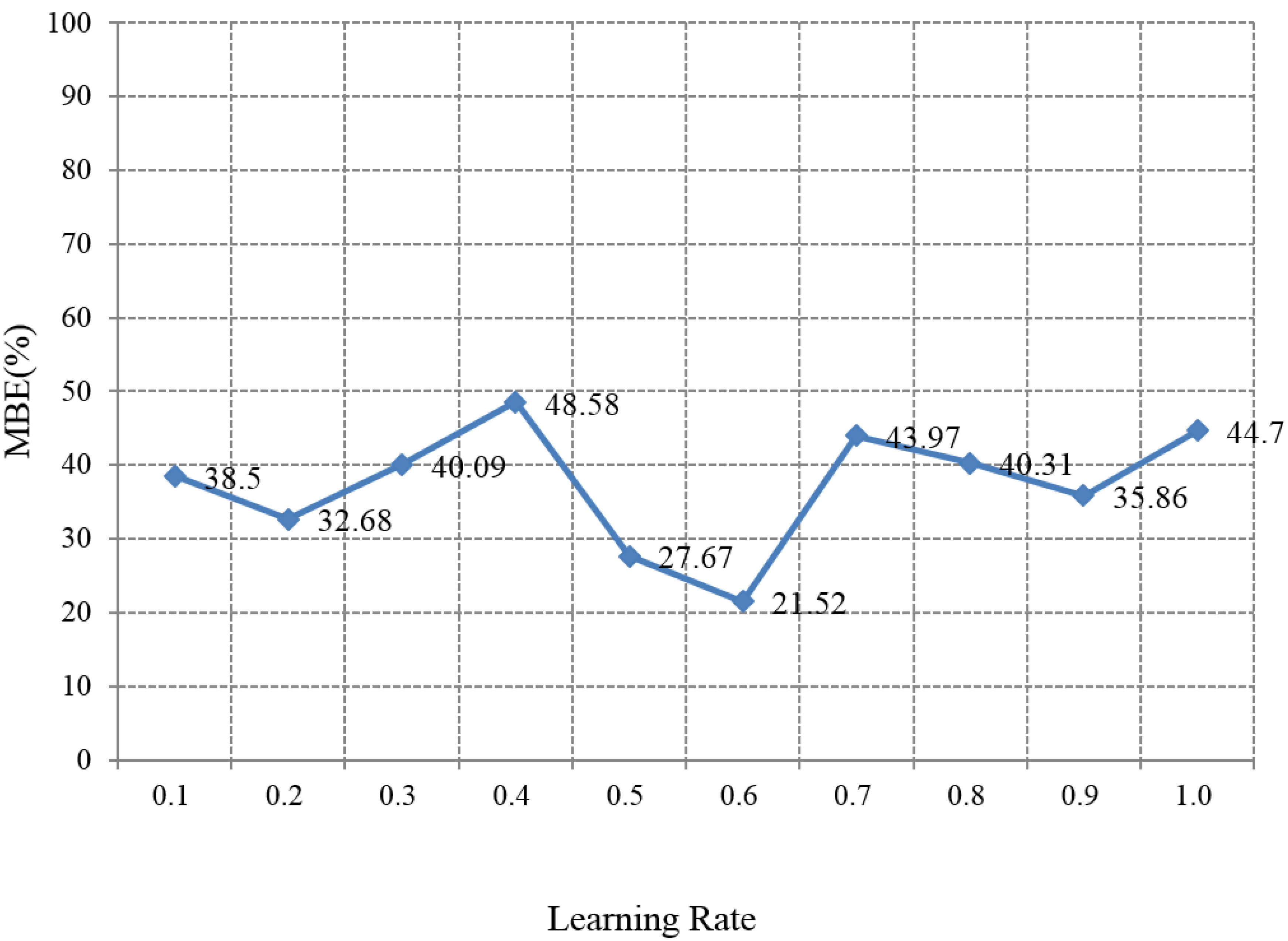
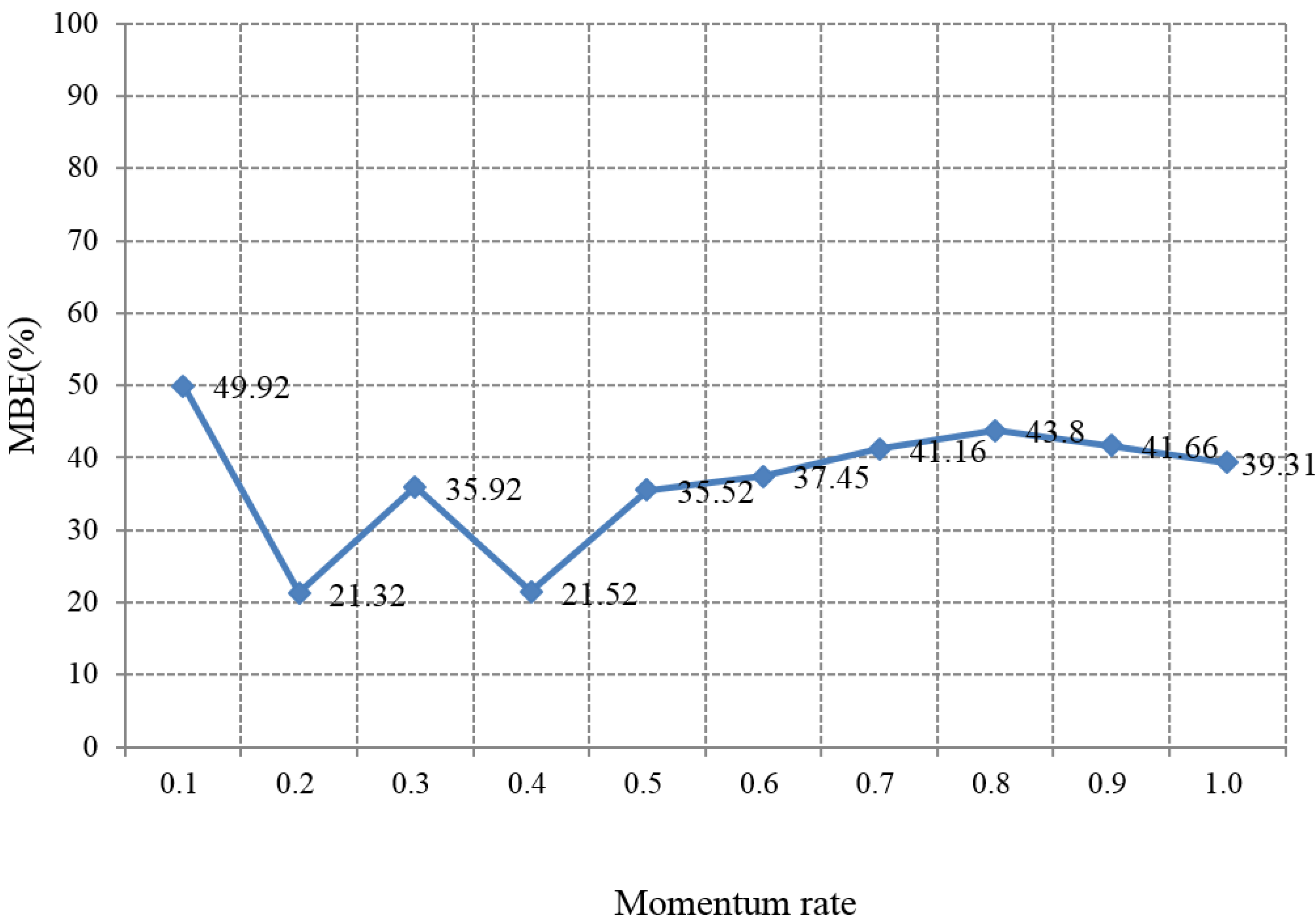
For optimizing the initial model, 100 datasets were prepared using the same method explained in Section 2.1, thus employing the simulation model from MATLAB and TRNSYS. The mean biased error (MBE, %) (Equation (1)) between the predicted values (S_i) and the simulated values (M_i) was calculated for each parametrical value, and the value that produced the smallest MBE was determined as the optimal value of the components.

Table 6. Parametrically tested values for optimizing the ANN components.

Components to be Optimized	Parametrical Values to be Tested
Number of hidden neurons	1	2	3	4	5	6	7	8	9	10
	11	12	13	14	15	16	17	18	19	20
Number of hidden layer	1	2	3	4	5	6	7	8	9	10
Learning rate	0.1	0.2	0.3	0.4	0.5	0.6	0.7	0.8	0.9	1.0
Momentum rate	0.1	0.2	0.3	0.4	0.5	0.6	0.7	0.8	0.9	1.0

Table 6. Parametrically tested values for optimizing the ANN components.

Components to be Optimized	Parametrical Values to be Tested
Number of hidden neurons	1	2	3	4	5	6	7	8	9	10
	11	12	13	14	15	16	17	18	19	20
Number of hidden layer	1	2	3	4	5	6	7	8	9	10
Learning rate	0.1	0.2	0.3	0.4	0.5	0.6	0.7	0.8	0.9	1.0
Momentum rate	0.1	0.2	0.3	0.4	0.5	0.6	0.7	0.8	0.9	1.0

$$\text{MBE}=\frac{{{\displaystyle \sum }}_{i=1}^n|S_{\text{i}}-M_{\text{i}}|}{{{\displaystyle \sum }}_{i=1}^n{M}_{\text{i}}}\times 100$$

(1)

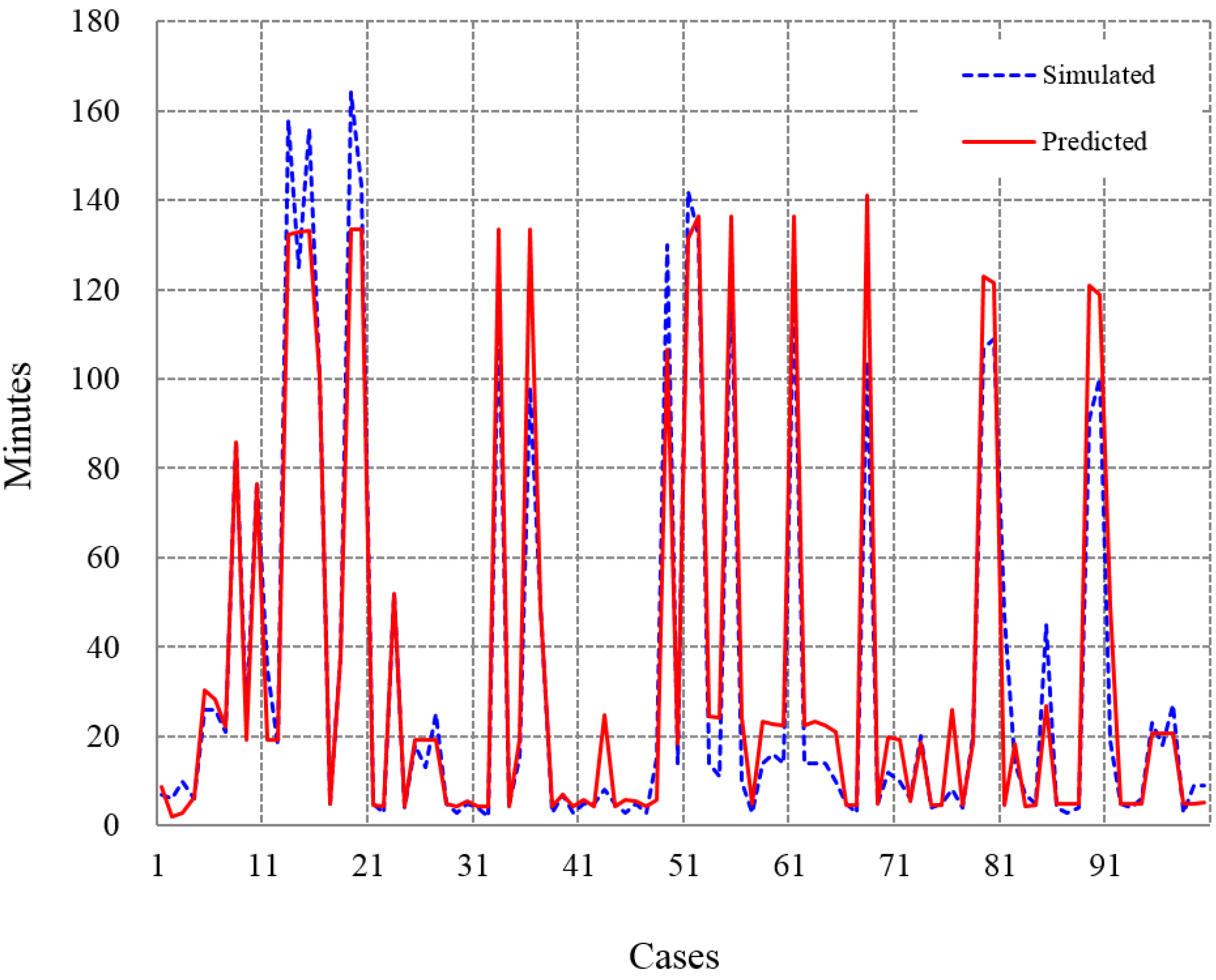
2.3. Evaluation of the Optimized ANN Model Performance

The optimized ANN model was tested in terms of its prediction performance. As in the optimization process, 100 datasets were prepared for the performance tests. Data were collected using the same simulation method that was used for collecting training and optimization datasets. Through the comparison of the predicted TIMP_SPT and the simulated TIMP_SPT using MBE, the prediction accuracy of the developed ANN model was validated. Thereafter, the developed ANN model could be applied in the control logic.

3. Results Analysis

3.1. Initial Structure of the Model

The statistical relationships between the input variables and the output variable of the ANN model are shown in Figure 8, Figure 9, Figure 10 and Figure 11 and summarized in Table 7. The ANOVA (analysis of variance) test results between each input variable and the required minutes for restoring the normal comfortable set-point temperature was calculated for investigating the statistical relationship.

The R² between TEMP_IN and the required minutes (Figure 8), between ΔTEMP_IN and the required minutes (Figure 9), between TEMP_DIF and the required minutes (Figure 10), and between TEMP_OUT and the required minutes (Figure 11) were 0.5988, 2E-5, 0.5988, and 0.3052, respectively. From the R² of each variable, three variables (TEMP_IN, TEMP_DIF, and TEMP_OUT) presented a relatively stronger relationship with the output variable. Thus, these three variables were selected as the input variables of the revised ANN model.

Figure 8. Relationship between the indoor temperature (TEMP_IN) and the required minutes for restoring from the current temperature to the normal set-point temperature.

Figure 8. Relationship between the indoor temperature (TEMP_IN) and the required minutes for restoring from the current temperature to the normal set-point temperature.

Figure 9. Relationship between the indoor temperature change (ΔTEMP_IN) and the required minutes for restoring from the current temperature to the normal set-point temperature.

Figure 9. Relationship between the indoor temperature change (ΔTEMP_IN) and the required minutes for restoring from the current temperature to the normal set-point temperature.

Figure 10. Relationship between the indoor temperature from the normal set-point temperature (TEMP_DIF) and the required minutes for restoring from the current temperature to the normal set-point temperature.

Figure 10. Relationship between the indoor temperature from the normal set-point temperature (TEMP_DIF) and the required minutes for restoring from the current temperature to the normal set-point temperature.

Figure 11. Relationship between the outdoor temperature (TEMP_OUT) and the required minutes for restoring from the current temperature to the normal set-point temperature.

Figure 11. Relationship between the outdoor temperature (TEMP_OUT) and the required minutes for restoring from the current temperature to the normal set-point temperature.

Table 7. ANOVA test result for prediction models between inputs and output variables.

Independent Variables	Unstandardized Coefficients		t	Sig.	ANOVA
	B	Std. Error			R2	F(1,54)	Sig.
TEMPIN	18.701	2.103	8.894	<0.001	0.599	79.097	<0.001
ΔTEMPIN	−3.214	50.919	−0.063	0.950	<0.001	0.004	0.950
TEMPDIF	18.701	2.103	8.894	<0.001	0.599	79.097	<0.001
TEMPOUT	10.354	2.145	4.827	<0.001	0.305	23.302	<0.001

Table 7. ANOVA test result for prediction models between inputs and output variables.

Independent Variables	Unstandardized Coefficients		t	Sig.	ANOVA
	B	Std. Error			R2	F(1,54)	Sig.
TEMPIN	18.701	2.103	8.894	<0.001	0.599	79.097	<0.001
ΔTEMPIN	−3.214	50.919	−0.063	0.950	<0.001	0.004	0.950
TEMPDIF	18.701	2.103	8.894	<0.001	0.599	79.097	<0.001
TEMPOUT	10.354	2.145	4.827	<0.001	0.305	23.302	<0.001

3.2. Optimization Results

Statistical analysis was conducted to determine the optimal ANN model components, and the results are shown in Figure 12, Figure 13, Figure 14 and Figure 15. The first step was to find the optimal number of hidden neurons that produced the least MBE between the predicted and numerically simulated values. In this step, the number of hidden layers, the learning rate, and the momentum rate were fixed as initially determined (1, 0.6, and 0.4, respectively). As shown in Figure 13, the MBE (%) ranged from 22.52 to 115.28% for the 1 to 20 hidden neurons. The least value was obtained when the ANN model employed four hidden neurons (22.52%) while the initial model with nine hidden neurons produced a slightly higher value (23.18%). Thus, the initial model changed its number of hidden neurons to four.

The second step was to optimize the number of hidden layers. The number of hidden layers was changed from 1 to 10, as shown in Figure 14, and the prediction results were compared to the simulation results. During this process, the number of hidden neuron was fixed as the determined optimal value, which was 4, and the other two components such as learning rate and moment were fixed as initial values. The MBE ranged 21.52% to 122.6% as the number of hidden layer was changed. The best case was when the 3-hidden layers were applied in the ANN model. Thus, the number of hidden neuron of the initial model was changed to 3.

Figure 12. MBE (mean biased error) values by number of hidden neurons.

Figure 12. MBE (mean biased error) values by number of hidden neurons.

Figure 13. Mean based error (MBE) values by number of hidden layers.

Figure 13. Mean based error (MBE) values by number of hidden layers.

Figure 14. MBE values by learning rate.

Figure 14. MBE values by learning rate.

Figure 15. MBE values by momentum rate.

Figure 15. MBE values by momentum rate.

The third step was conducted for finding the optimal learning rate of the ANN model. For this, the learning rate was parametrically changed from 0.1 to 1.0, as indicated in Figure 14. The number of hidden neurons and hidden layers were assigned as 4 and 3, respectively, which were found to be the optimal values in the previous two steps, and the momentum rate was 0.4 as an initial value. As shown in Figure 15, the optimal value for the learning rate was found to be 0.6, with a 21.52% MBE. Thus, the revised model had a 0.4 learning rate.

The last step was for optimizing the value of the moment. As in the previous step, the moment was changed from 0.1 to 1.0 in Figure 15. At this step, the number of hidden neurons, the number of hidden layers, and the learning rate were fixed as optimal values found at steps 1 to 3. When comparing the MBE of the ANN model with a different moment, the least MBE was produced from a model with 0.2 momentum rate. The amount of MBE was 21.32%; thus, the optimal momentum rate was determined to be 0.2. Based on the four steps conducted for finding the optimal ANN components, the optimal ANN model was determined to have four hidden neurons, three hidden layers, a 0.6 learning rate, and 0.2 momentum rate.

3.3. Prediction Performance of the Optimized Model

The optimized ANN model was evaluated its performance in terms of prediction accuracy. 100 datasets were newly collected from the simulation model and they were compared with the calculated data from the ANN model. Figure 16 compares the data obtained from the use of the simulation model (blue dotted line) and the prediction data from the ANN model (red solid line). The y-value of the chart means the time in minutes required for changing the current temperature to the set-point temperature.

Figure 16. Comparison of the simulation and prediction results.

Figure 16. Comparison of the simulation and prediction results.

As shown in the figure, the predicted time from the ANN model followed the simulated time. For the 100 cases, the average difference between the simulation and the prediction results was 7.56 min. The maximal and minimal minutes were 164.0 and 2.0, respectively, for the simulation results, and 141.09 and 2.09 for the prediction results from the ANN model.

The MBE between the simulation and prediction results was 21.90%, which was less than 25%. Based on the previous study, which proposed 10%–25% or around 25% as a statistically meaningful value for supporting the applicability of the model [26], the prediction accuracy of the developed ANN model with 21.90% MBE was validated. Thus, the applicability of the ANN model to the control logic was proven.

4. Conclusions

This study aimed at developing an artificial-neural-network (ANN)-based model that can calculate the required time for changing the current indoor temperature to the normal set-point temperature (TIMP_SPT) in the cooling season. By applying the calculated time in the control logic, the operation of the cooling system can be predetermined to condition the indoor temperature comfortably in a more energy-efficient manner. Three major steps were carried out for developing and optimizing an ANN model, and for testing its prediction performance. The MATLAB and TRNSYS software were employed in an incorporative manner in the development process. The findings from the three major steps are summarized below.

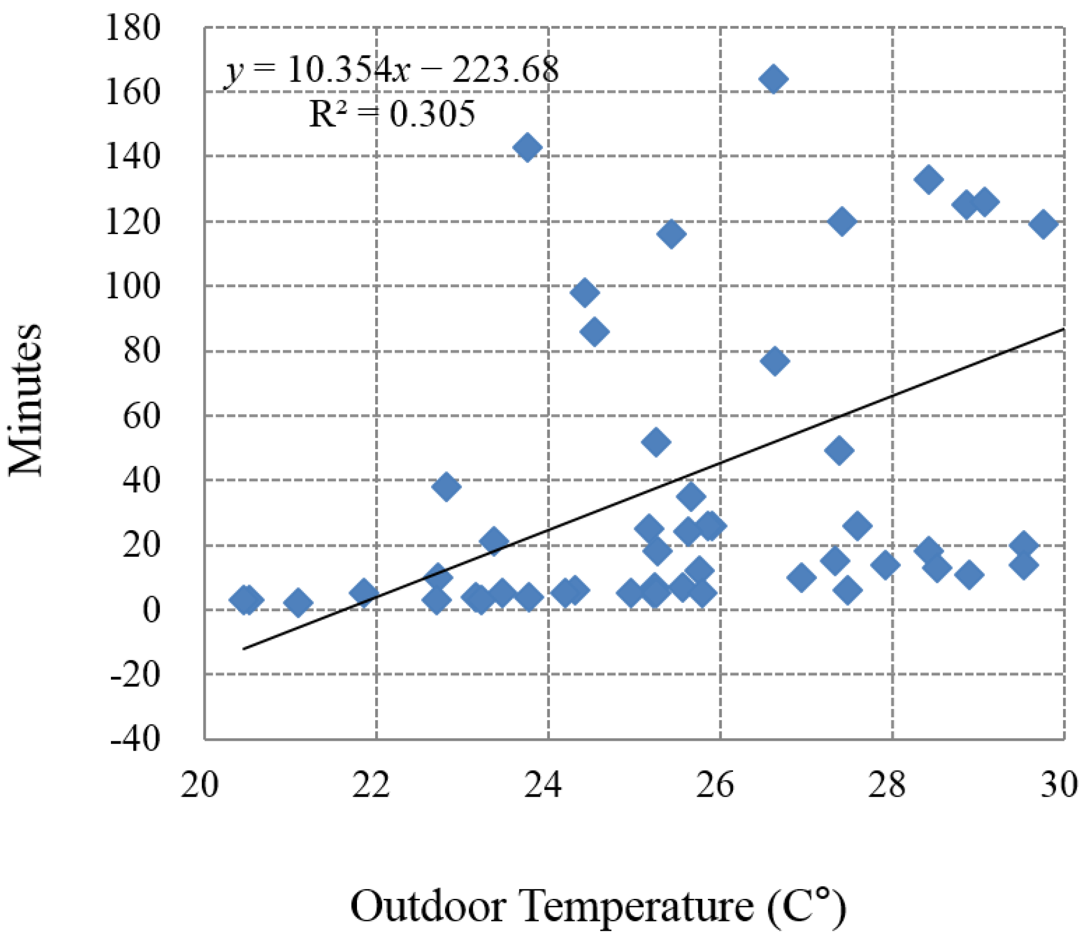
(1) Through the statistical analysis of the relationship between the input neurons and the output neuron, the R² between TEMP_IN and TIMP_SPT, between TEMP_DIF and TIMP_SPT, and between TEMP_OUT and TIMP_SPT were relatively higher. Thus, the initial ANN model was determined to have these three variables as the input variables.

(2) Through the parametrical analysis of the prediction performance of the initial ANN model, the initial ANN model, which presented the least MBE between the simulation and prediction results, was modified to have four hidden neurons, three hidden layers, a 0.6 learning rate, and a 0.2 momentum rate.

(3) In the tests that measured the performance of the optimized ANN model in terms of prediction accuracy, the optimized ANN model presented a lower MBE under generally accepted levels. Thus, the developed ANN model was proven to have the potential to be applied to the thermal control logic.

From the development process employed in this study, the optimized ANN model showed prediction accuracy and applicability to the control logic for determining the optimal start moment of the cooling system during the setback period in accommodation buildings. Further study is warranted to test the performance of the thermal control logic after applying the ANN model developed in this study. The numerical computer simulation method as well as application to real buildings needs to be considered to test the model’s performance. In addition, the ANN model and thermal control logic for the heating system will be developed in the future study. Based on synthetic control logic application, the indoor thermal environment of accommodation buildings will be conditioned more comfortably and in a more energy-efficient manner.