Failures during Load-Frequency Control Maneuvers in an Upgraded Hydropower Plant: Causes, Identification of Causes and Solution Proposals

Abstract

The objective of this paper is to investigate the cause of several unexpected high amplitude oscillations that occurred in the surge tank water level of a real hydropower plant during secondary load-frequency control (LFC) maneuvers, after the replacement of the turbine runner, and to propose solutions that allow the power plant to continue providing secondary LFC in a safe and reliable manner. For this purpose, a simulation model has been developed and calibrated from data gathered during several on-site tests. Two different solutions are proposed in order to cope with the observed problem: using a state-dependent load change rate limiter or modifying the hydro turbine governor gains; the turbine governor remains the same as before the runner replacement. The proposed solutions are tested against a set of realistic secondary LFC signals by means of simulations and compared to each other as a function of the probability that the surge tank water level descends below a minimum safe level and the quality of the secondary LFC response. The results presented in the paper demonstrate the validity of the methodology proposed to determine the state-dependent ramp limit, as well as its effectiveness to prevent the surge tank drawdown and to provide clear insight into the trade-off between response quality and power plant safety.

1. Introduction

During the last few decades, renewable energies experienced a continuous growth. In Europe, this growth was promoted by several European directives, as well as by the corresponding country regulations. The advantages of renewable energies are obvious. However, the non-dispatchable nature of some of these energies, such as solar and wind, may pose some important problems for power system operation [1].

Amongst all renewable energy sources, wind is the one that experienced a bigger growth during last decade. Besides its non-dispatchable nature, wind power has a strong variability; as stated in [2], the power output of a wind farm may decrease from 100% down to 10% within 6 min. 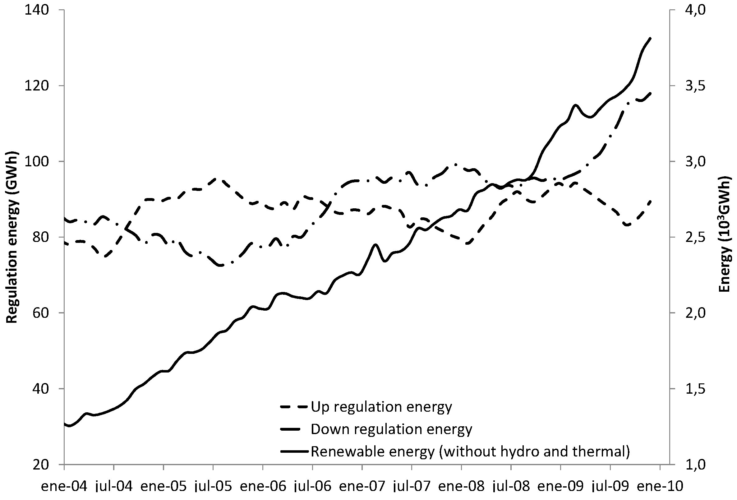Despite their obvious advantages, the integration of non-dispatchable energies into the power system may increase the need for balancing services [3,4]. In Spain, the installed wind power capacity grew from 6160 MW at the end of 2003 to 22,739 MW at the end of 2013. As can be seen in Figure 1, the increase in the contribution of renewable energies to the electric power supply in Spain came accompanied by a considerable increase in the energy required for providing secondary load-frequency control (LFC), especially for down-regulation.

Figure 1. Moving average of up- and down-regulation energy and renewable energy production in the Spanish power system.

Figure 1. Moving average of up- and down-regulation energy and renewable energy production in the Spanish power system.

As is well known, hydropower plants have excellent skills for providing balancing services, thus contributing to the integration of non-dispatchable energy into the power system [5,6]. However, in most industrialized countries, there exist important environmental barriers, usually in the form of more and more environmental requirements every day, to the construction of new hydropower reservoirs [7]. As a consequence of these and other barriers, the hydropower sector in industrialized countries is mainly focused on the upgrading and optimization of existing hydro plants, as well as on the use of existing reservoirs associated with other uses, such as drinking water supply or irrigation, for hydropower purposes [6].

Simulation models help gain insight into the dynamic response of a hydropower plant and to better understand the physical phenomena involved in the plant’s dynamic behavior [8]. Hydropower plant’s simulation models have been used for different purposes in the technical literature. In [9,10], a simulation model was developed for the study of hydraulic transients in a hydropower plant. In [11], a simulation model was used for the design of the control algorithms of a new hydropower plant. In [8], a simulation model was developed to analyze the cause of an unexpected oscillatory behavior in the power output of a pumped-storage power plant.

As stated in [12], simulation models play an important role in the upgrading process of old hydropower plants. In [13], simulation was used for the design of an automatic water level control system in a low-head small hydropower plant that had been refurbished several years ago. In [14], a simulation model was developed to assist the design of different control algorithms of the Reisseck-Kreuzeck hydro plant, in Austria, after the replacement of the outdated mechanical governors by new digital controllers.

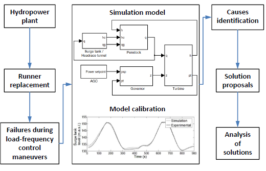
In this paper, a simulation model is developed to investigate the cause of several unexpected high amplitude oscillations that occurred in the surge tank water level (STWL) of a real hydropower plant during secondary LFC maneuvers, as well as to propose solutions that allow the plant to continue providing secondary LFC in a safe and reliable manner.

The hydropower plant analyzed in the paper is located in the northwest area of Spain and is composed of an upper reservoir, a head-race tunnel, a surge tank, a penstock and a single Francis turbine. The main design parameters of the hydropower plant can be found in the Appendix. Recently, the turbine runner was replaced by a new one, with a greater rated flow, with the purpose of increasing the installed power capacity, whereas the turbine governor remains the same as before the runner replacement. After the runner replacement, the amplitude of the water level oscillations that appear in the surge tank when the power plant is tracking the power set-point signals of the automatic generation control system (AGC) has increased in a degree considerably greater than expected; so much so that several load rejections occurred in order to prevent air from entering the penstock and then the turbine.

The oscillations that appear in the STWL as a consequence of sudden start-up or shut-down maneuvers were studied in [9,15]. Nevertheless, the oscillations that occur in the surge tank when the power plant is providing secondary LFC have not received special attention in the technical literature, probably since, traditionally, sudden start-up and shut-down maneuvers have been used as the worst large disturbances to be considered for the design and other purposes [15].

The primary LFC loop has received more attention in the literature on hydropower control. The influence of the turbine governor gains on the stability of the primary LFC loop of a hydropower plant was further studied several years ago [16,17,18]; most of these stability studies were carried out on the basis of a small disturbance analysis [15]. Secondary LFC maneuvers can be hardly considered small disturbances. Their magnitude can be as large as the whole power range of the hydropower plant; i.e., maximum minus minimum power. The response time of the secondary LFC loop is one or several orders of magnitude longer than that of the primary one. The dynamics of the secondary LFC loop may therefore couple with that of other elements of the power plant with similar time constants, such as the surge tank. For these reasons, it seems obvious that the secondary LFC loop response should not be studied on the basis of a small disturbance analysis, but with the help of non-linear simulation models [19].

As can be seen in [20], the reserve response capacity of a hydropower plant strongly depends on the power plant operating point, the turbine governor gains and the time evolution of the power reserve requests. As stated in that paper, it is in general possible to tune the turbine governor settings in such a way that the power plant safety is guaranteed, albeit at the expense of a reduced response quality or capacity. The trade-off between the quality of the secondary LFC response and the power plant safety (measured from the probability of occurrence of the surge tank drawdown) is analyzed in a recently upgraded hydropower plant, where the room for trade-off solutions has considerably diminished.

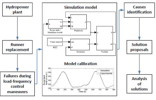
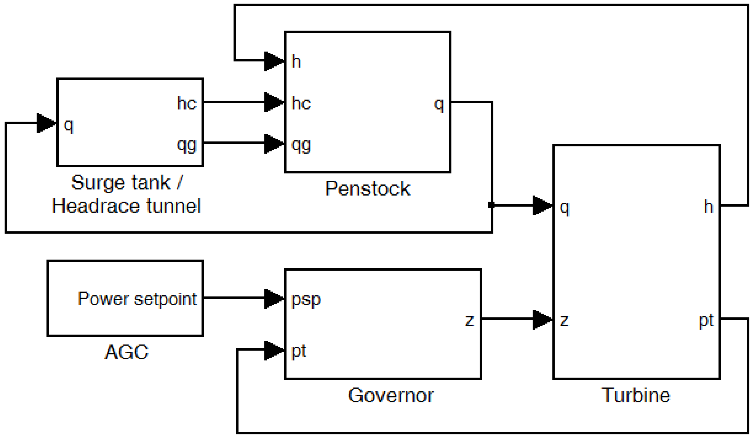
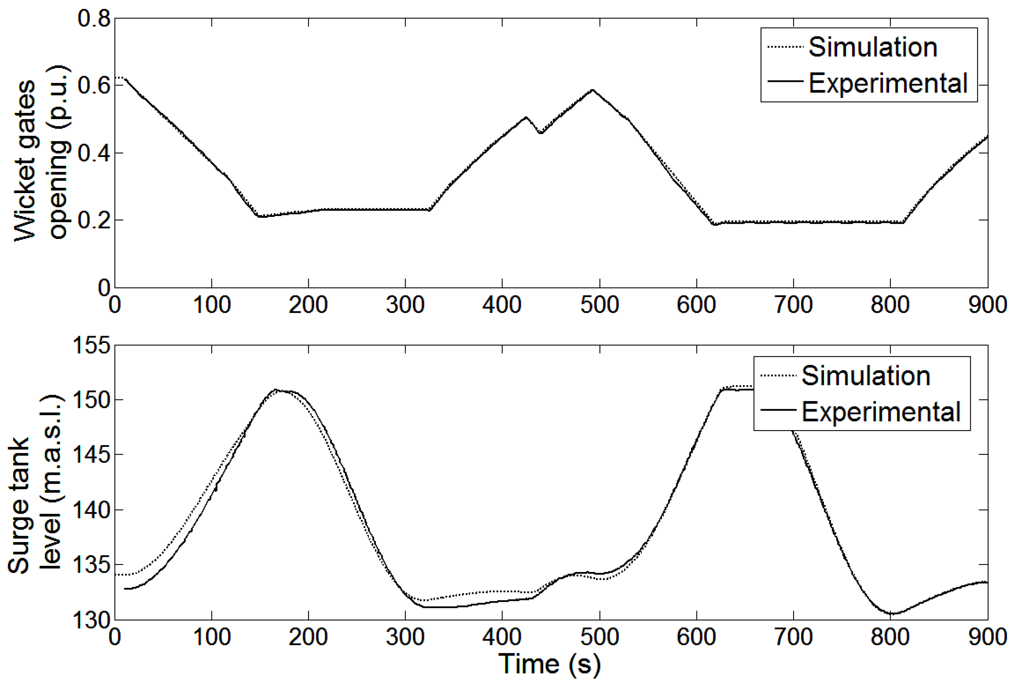
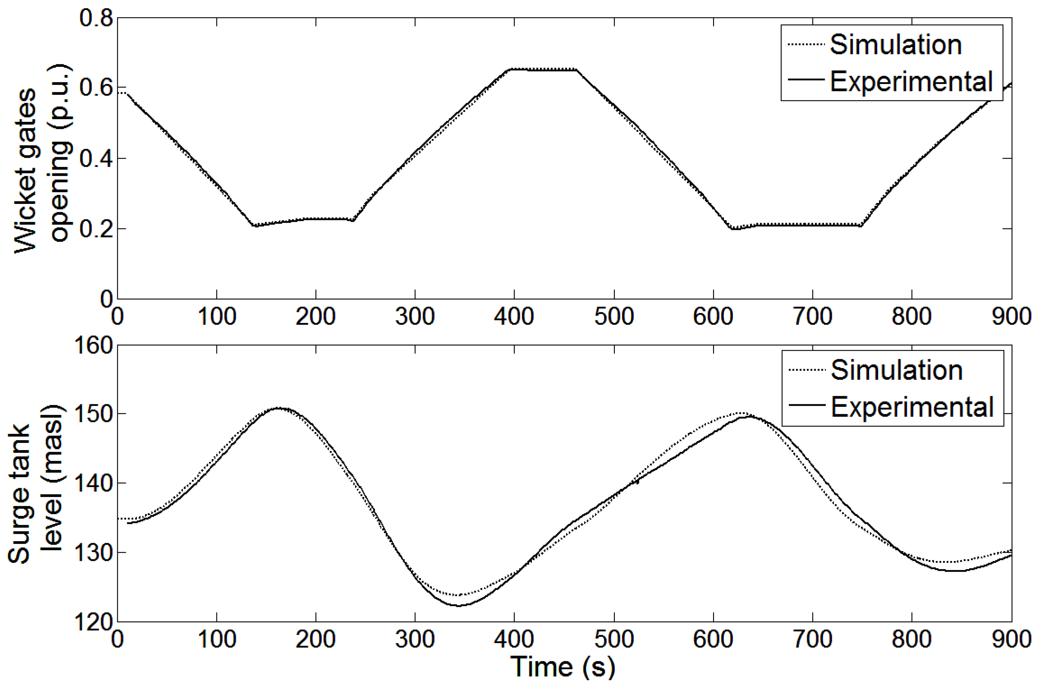
The rest of the paper is organized as follows. In Section 2, the simulation model used to pursue the above-mentioned objective is described in detail. In Section 3, the procedure followed to calibrate the model parameters is outlined. In Section 4, the cause of the high amplitude oscillations in the STWL is identified. In Section 5, two different solutions are proposed to alleviate the problem. Solutions are compared to each other as a function of both the quality of secondary LFC response and the probability that the STWL descends below a certain level. The main conclusions of the paper are duly drawn in Section 6.

2. Simulation Model

The model developed to pursue the above-mentioned objective is described in this section. The block diagram of the model is shown in Figure 2. The model is similar to the one presented in [21]. Nevertheless, for the sake of clarity, the main aspects of the model are described in the following subsections.

2.1. Surge Tank/Head Race Tunnel

The head-race tunnel joins the upper reservoir and surge tank together. A rigid water column model is used to represent its behavior (Equation (1)). Continuous friction losses in the conduit are modeled using the Manning-Strickler expression. Additionally, several local head losses that occur in the junction among the surge tank, head-race tunnel and penstock, as well as in the junction between the main body and upper chamber of the surge tank are modeled through different coefficients, according the flow direction (Figure 3):

$$\begin{array}{l}\frac{\text{d}{q}_{\text{g}}}{\text{d}t}=\left(h_{\text{00}}-h_{\text{c}}-\frac{r_{\text{g}}}{2}{q}_{\text{g}}|q_{\text{g}}|-\left(\frac{r_{\text{loc\_gen}}}{2}+\frac{r_{\text{loc\_s}}}{2}\right)(q_{\text{g}}-q)|q_{\text{g}}-q|\right)\frac{1}{T_{\text{g}}}\\ \text{if\hspace{0.17em}\hspace{0.17em}}\{\begin{array}{c}q<q_{\text{g}}\to r_{\text{loc\_gen}}=r_{\text{loc}};r_{\text{loc\_s}}=r_{\text{locsup}}\\ q>q_{\text{g}}\to r_{\text{loc\_gen}}=r_{\text{locd}};r_{\text{loc\_s}}=r_{\text{locsdw}}\\ q=0\to r_{\text{loc\_gen}}=r_{\text{locdisp}}\end{array}\text{\hspace{0.17em}\hspace{0.17em}\hspace{0.17em}\hspace{0.17em}\hspace{0.17em}\hspace{0.17em}\hspace{0.17em}and\hspace{0.17em}\hspace{0.17em}if\hspace{0.17em}\hspace{0.17em}\hspace{0.17em}\hspace{0.17em}\hspace{0.17em}\hspace{0.17em}}{h}_{\text{c}}<h_{\text{csup}}\to r_{\text{loc\_s\hspace{0.17em}}}=0\end{array}$$

(1)

Figure 2. Block diagram of the simulation model. AGC: automatic generation control system.

Figure 2. Block diagram of the simulation model. AGC: automatic generation control system.

The surge tank of the power plant under study is divided into three parts: the upper chamber, main body and lower chamber. Local head losses between the upper chamber and main have been considered through coefficients r_locsup and r_locsdw. Local head losses between the head-race tunnel and lower chamber and between the lower chamber and main body are considered altogether through coefficients r_loc and r_locd. The results obtained during the calibration procedure (Section 3) indicated that it is not necessary to use different coefficients for each cross-section change. Furthermore, there is a relay right at the joint between the lower chamber and main body of the surge tank, which is in charge of provoking a load rejection whenever the STWL decreases below its position; splitting the above-mentioned coefficients lacks therefore interest for the purposes of the study.

Figure 3. Local head loss coefficients in the surge tank.

Figure 3. Local head loss coefficients in the surge tank.

The surge tank dynamics is modeled as follows:

$$\frac{\text{d}{h}_{\text{c}}}{\text{d}t}=\left(q_{\text{g}}-q\right)\frac{1}{T_{\text{c}}\left(h_{\text{c}}\right)}$$

(2)

where T_c is the time or storage constant of the surge tank [22], which depends on the surge tank cross-section area and, thus, on the water level h_c.

2.2. Penstock

As stated in [10], the length of the penstock is a key factor for considering the elasticity of the conduit and the compressibility of water; the longer the penstock, the more important it is to consider these factors. Since the hydropower plant modeled in this work presents a short penstock, a rigid water column approach has been used to model its behavior (Equation (3)). Both continuous friction losses and local head losses are considered in an analogous way to Equation (1):

$$\begin{array}{l}\frac{\text{d}q}{dt}=\left(h_{\text{c}}-h-\frac{r}{\text{2}}q|q|-\left(\frac{r_{\text{loc\_gen}}}{\text{2}}+\frac{r_{\text{loc\_s}}}{\text{2}}\right)(q-q_{\text{g}})|q-q_{\text{g}}|\right)\frac{1}{T_{\text{a}}}\\ \text{if\hspace{0.17em}\hspace{0.17em}}\{\begin{array}{c}q>q_{\text{g}}\to r_{\text{loc\_gen}}=r_{\text{locd}};r_{\text{loc\_s}}=r_{\text{locsup}}\\ q<q_{\text{g}}\to r_{\text{loc\_gen}}=r_{\text{loc}};r_{\text{loc\_s}}=r_{\text{locsdw}}\\ q=0\to r_{\text{loc\_gen}}=r_{\text{locdisp}}\end{array}\text{\hspace{0.17em}\hspace{0.17em}\hspace{0.17em}\hspace{0.17em}\hspace{0.17em}\hspace{0.17em}\hspace{0.17em}\hspace{0.17em}and\hspace{0.17em}\hspace{0.17em}if\hspace{0.17em}\hspace{0.17em}\hspace{0.17em}\hspace{0.17em}}{h}_{\text{c}}<h_{\text{csup}}\to r_{\text{loc\_s\hspace{0.17em}}}=0\end{array}$$

(3)

2.3. Turbine and Governor

The turbines have been modeled according to Equations (4)–(6), following the recommendations of [22]. In a similar way to [23,24], original expressions proposed in [22] were slightly modified according to the measurements obtained in a series of on-site tests. Unlike [22], Equation (5) does not comprise a second term depending on the unit speed deviations, since system frequency deviations are not explicitly considered in this paper. It should be noted that this paper is focused on STWL oscillations of significant amplitude, caused by large load variations, such as those requested for providing secondary LFC. In order to reproduce such STWL oscillations, the unit power set-point sent by the AGC system, psp, is used as a model input variable; it would not make sense to model the power system frequency deviation or LFC in response to such “artificially”-generated unbalances. Modelling the AGC system and the Spanish mainland power system frequency and LFC is outside the scope of this paper (see [21] for a small power system model with these features).

$$q=z\frac{1}{K_{\text{z}}}\sqrt{\text{h}}$$

(4)

$$p_t=\eta (h,q)·h·q$$

(5)

$$\eta (h,q)=a+b{h}^2+c{q}^2$$

(6)

A conventional proportional-integral controller processes the power-frequency error signal, Pfe, and sends a control signal (CS) to a servomotor, which modifies the wicket gates’ position. The expressions used to model the behavior of the speed governor are summarized in Equations (7)–(9); the speed term of the power-frequency error Equation (7) can be neglected, since as it was mentioned above that speed deviations are not considered in the paper. The diagram of the governor sub-block is shown in Figure 4. Both the speed and position of the wicket gates are limited by means of a rate limiter and saturation blocks:

$$Pfe=\Delta n+\text{σ}\Delta p=\left(n_0-n\right)-\text{σ}\left(psp-p_t\right)=-\text{σ}\left(psp-p_t\right)$$

(7)

$$\left(K_{\text{p}}+K_{\text{i}}{\displaystyle \int \text{d}t}\right)Pfe=CS$$

(8)

$$\frac{\text{d}\Delta z}{\text{d}t}=\frac{1}{T_{\text{s}}}\left(CS-\Delta z\right)$$

(9)

Figure 4. Block diagram of the turbine governor.

Figure 4. Block diagram of the turbine governor.

3. Model Calibration

The parameters of the above-described simulation model were calibrated from data gathered during a series of on-site tests. Specifically, the data calibrated are: (i) continuous and local head loss coefficients; (ii) coefficients a, b and c (Equation (6)); (iii) discharge coefficient K_z (Equation (4)); and (iv) proportional and integral gains of the turbine governor, K_p and K_i.

Continuous head loss coefficients, as well as turbine efficiency and discharge coefficients were calibrated from steady-state tests. Local head losses coefficients were calibrated from both load variation and rejection maneuvers. Load variation maneuvers were done in open-loop [25]. Several profiles of wicket gates opening versus time were designed from a preliminary simulation study, in order to force the water in the surge tank to both reach the upper chamber and to provoke a load rejection to prevent air from entering the penstock; load rejections from both steady and unsteady states were therefore tested. Water time constants T_g, T_c, T_a were calculated from data included in the construction project documents. In Figure 5 and Figure 6, the evolution of the STWL during a load variation test is simulated and compared to the on-site measurements. Proportional and integral gains of the turbine governor were fitted from a few data gathered during closed-loop operation. The numerical values of all calibrated parameters are included in Table 1.

Table 1. Values of calibrated parameters.

Parameter	Value	Parameter	Value	Parameter	Value
rloc	0.0397	r	0.1241	Kz	0.9217
rlocd	0.1241	rg	0.1937	a	0.9323
rlocsup	0.0005	Kp	2.8571	b	−0.2645
rlocsdw	0.0005	Ki	0.9524	c	0.1798

Table 1. Values of calibrated parameters.

Parameter	Value	Parameter	Value	Parameter	Value
rloc	0.0397	r	0.1241	Kz	0.9217
rlocd	0.1241	rg	0.1937	a	0.9323
rlocsup	0.0005	Kp	2.8571	b	−0.2645
rlocsdw	0.0005	Ki	0.9524	c	0.1798

Figure 5. Comparison of recorded and simulated wicket gate opening and surge tank water level (on-site Test 1).

Figure 5. Comparison of recorded and simulated wicket gate opening and surge tank water level (on-site Test 1).

Figure 6. Comparison of recorded and simulated wicket gate opening and surge water tank level (on-site Test 2).

Figure 6. Comparison of recorded and simulated wicket gate opening and surge water tank level (on-site Test 2).

4. Identification of the Problem

As was mentioned above, the turbine runner of the power plant under study was recently replaced by a new one, with the purpose of increasing the installed power capacity. As is discussed in [26], the change in rated flow entails certain changes in the power plant dynamics; water starting time both in the penstock and head-race tunnel, as well as surge tank time constant vary as a function of the rated flow. In addition, the increase in rated power may be accompanied by an increase in the power regulation range, and consistently, an increase in the amplitude of the oscillations in the STWL is not surprising, provided that the turbine governor remains the same as before the runner replacement. 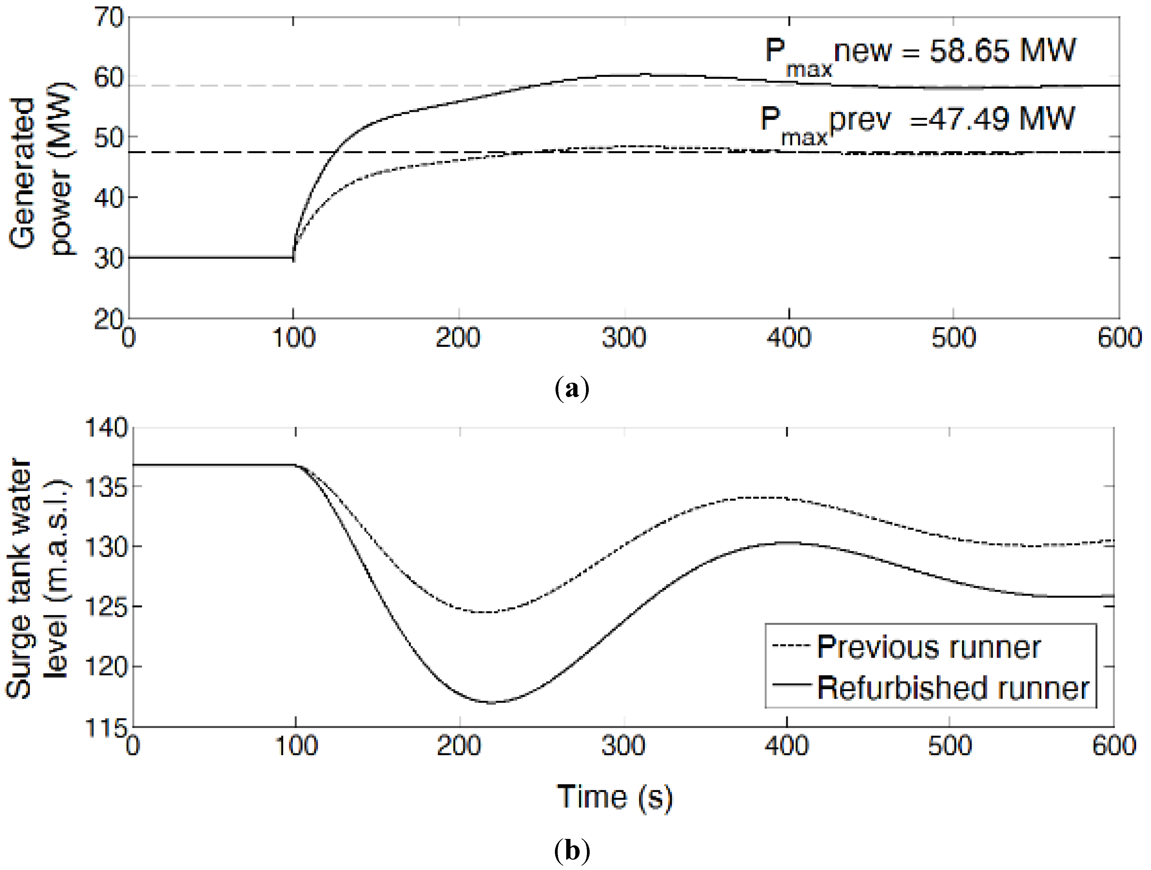In Figure 7, the evolution of output power and STWL in response to a ramp power set-point signal have been depicted before and after the runner replacement. The initial output power and ramp slope are identical in both simulations. The power set-point signal goes in both cases from initial output power to maximum power (47.49 MW and 58.65 MW before and after the runner replacement, respectively). As expected, the amplitude of the oscillations in the STWL is higher with the new runner, as a consequence of the greater ramp duration and magnitude.

Theoretically, the worst single maneuver would be the turbine start-up with the minimum water level in the reservoir and maximum wicket gate opening rate. However, the fact is that the recorded load rejections were never caused by such a type of maneuver, but rather they occurred a long time after the unit start-up, when the power plant was tracking the AGC power set-point signal.

Figure 7. Evolution of (a) output power and (b) surge tank water level, with the old and new runner, in response to a ramp power set-point signal.

Figure 7. Evolution of (a) output power and (b) surge tank water level, with the old and new runner, in response to a ramp power set-point signal.

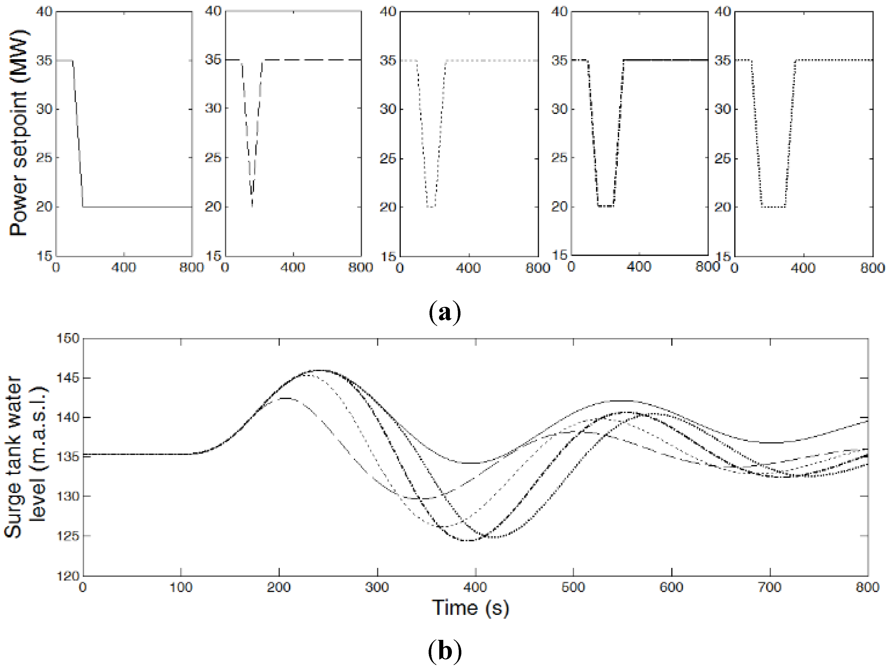
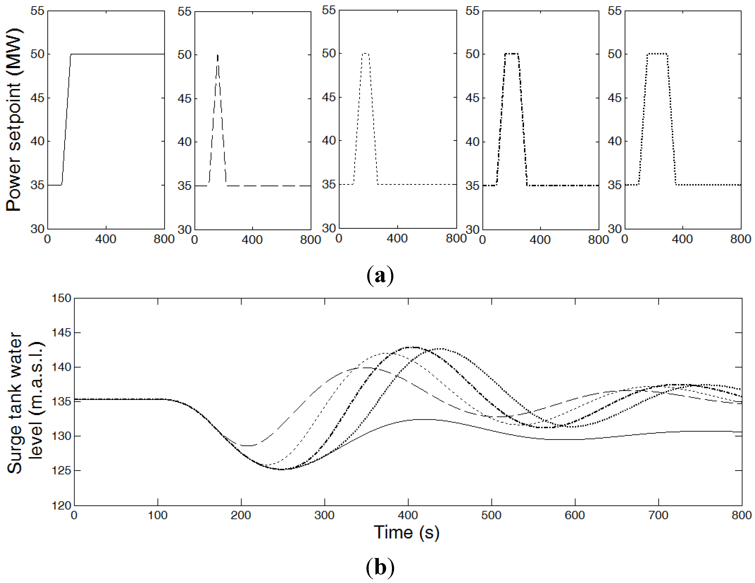
After a careful analysis, it was observed that, as glimpsed in [20], certain sequences of power set-point signals provoked a sort of resonance phenomenon in the STWL, amplifying to some extent the oscillation amplitude. In order to better understand this phenomenon, the evolution of STWL in response to different sequences of power set-point ramp signals has been depicted in Figure 8 and Figure 9 (b), along with the corresponding power set-point signals (a). For the sake of simplicity, only two ramp signals with the same magnitude and slope (in absolute value) have been simulated. As can be observed from the figures, the time elapsed between the end of the first ramp and the beginning of the second one (hereinafter referred to as ET), significantly influences the degree to which the oscillation amplitude is amplified and, therefore, the minimum STWL. Additionally, it can be deduced from the figure that the relation between ET and the oscillation amplitude is not linear, but rather there is an ET for which the oscillation amplitude is maximal.

Figure 8. Evolution of the surge tank water level in response to different sequences of down- and up-ward power set-point ramp signals: (a) sequences of power set-point signals; (b) evolution of the furge tank water level in response to the power set-point signals.

Figure 8. Evolution of the surge tank water level in response to different sequences of down- and up-ward power set-point ramp signals: (a) sequences of power set-point signals; (b) evolution of the furge tank water level in response to the power set-point signals.

Figure 9. Evolution of the surge tank water level in response to different sequences of up- and down-ward power set-point ramp signals: (a) sequences of power set-point signals; (b) Evolution of the surge tank water level in response to the power set-point signals.

Figure 9. Evolution of the surge tank water level in response to different sequences of up- and down-ward power set-point ramp signals: (a) sequences of power set-point signals; (b) Evolution of the surge tank water level in response to the power set-point signals.

5. Proposal of Solutions

Once the cause has been partially identified, the challenge is to propose solutions that allow the plant to continue offering as much power regulation range as possible for the secondary LFC in a safe and reliable manner. The ideal solution would be guaranteeing that the power set-point signals sent by the AGC will never provoke the above-described resonance phenomenon. As is well known, the AGC system is in charge of restoring the system frequency and reestablishing the power exchanges between areas to their scheduled values after any unexpected unbalance between generation and demand [27,28]. For these purposes, the AGC system computes the so-called area control error (ACE), as a function of both the frequency and power exchange errors, and generates and sends control signals to the synchronized units with the aim of eliminating the ACE. The profile of these signals mainly depends on the so-called area control error and on the AGC control algorithm, which makes the ideal solution practically unattainable. The “second best” solution would be guaranteeing that even though the AGC signals may amplify the oscillations amplitude, the STWL will never decrease below a minimum safe level (MSL). For this purpose, it would be necessary to first identify the sequences of AGC signals that make the water in the surge tank descend below the MSL and then act on the AGC signal or the turbine governor in order to guarantee that the identified sequences will not provoke an excessive drawdown of the surge tank.

In order to adopt this solution, it was necessary to make an assumption in such a way that the problem remains tractable. As is obvious, assuming sequences of ramp signals, of equal magnitude and slope (in absolute value), not only the ET influences the oscillation amplitude, but also the number of power set-point ramp signals. The greater the number of ramp signals, “properly” separated from each other (in time), the higher the oscillation amplitude. As is well known, AGC systems send power set-point signals in an almost continuous way, and thus, identifying a single sequence does not make much sense. Fortunately, the AGC signals seldom follow a specific ramp sequence pattern, and therefore, the appearance of the above-mentioned resonance phenomenon is not very likely, though possible, as demonstrated by the recorded events. The assumption adopted in this paper, in agreement with the power plant operator, in order to identify the worst likely sequences of AGC signals, is that such sequences are composed of two ramp signals of the same magnitude and slope in absolute value, the first one downward and the second one upward; as can be seen in Figure 8 and Figure 9, the downward-upward sequence makes the surge tank water decrease down to a lower value.

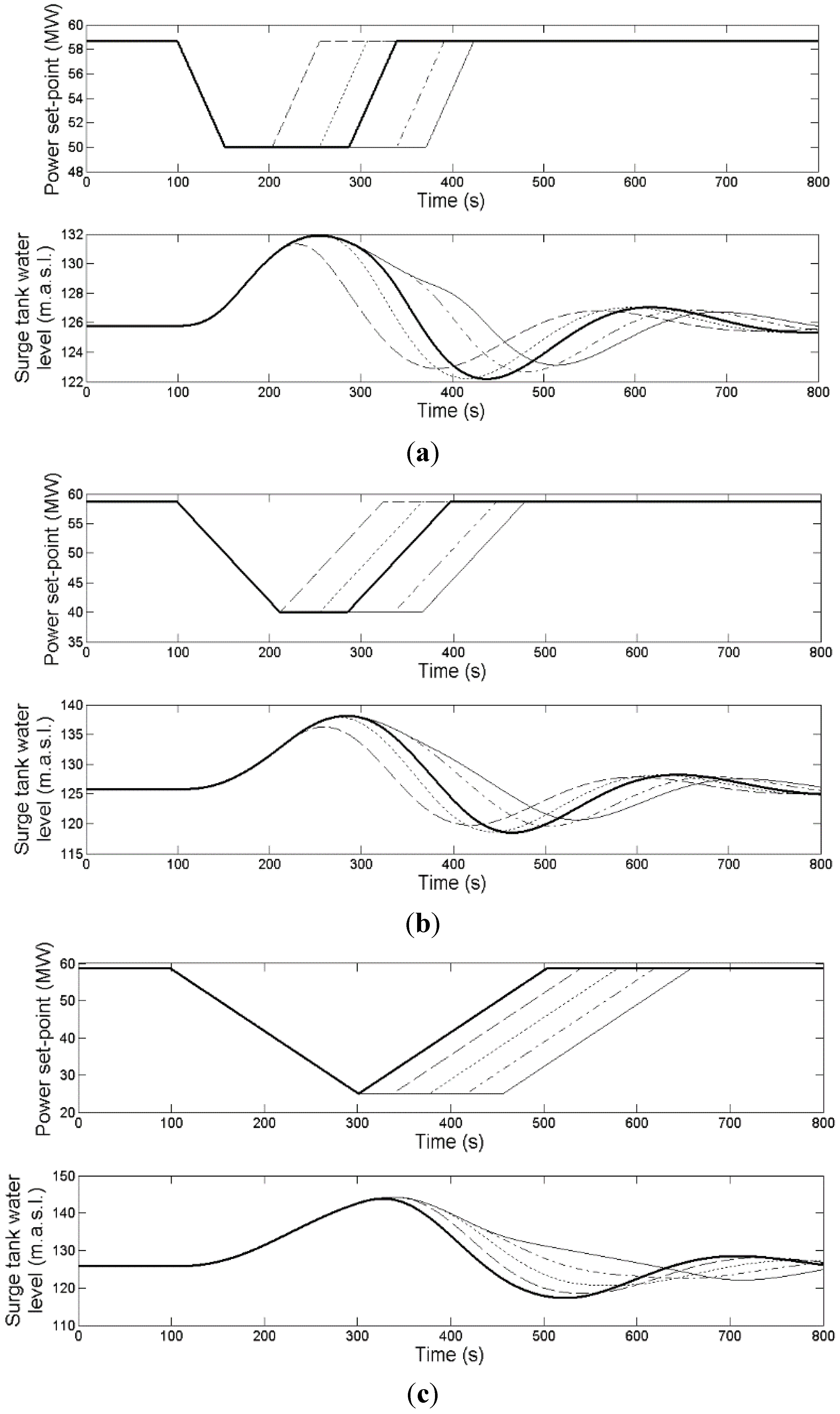
Once this assumption was adopted, several simulations were carried out varying the ramp slope (RS), the magnitude or duration (hereinafter referred to as RD), ET and the initial operating conditions (always in steady state). From the results of these simulations, it was concluded that for given initial operating conditions, the worst ET (WET) depends on the relation between RD and the period of the oscillations in the STWL (hereinafter referred to as SOT), as follows (Figure 10a–c).

-

If RD is shorter than or equal to SOT/4, WET is such that the second ramp finishes right at the time in between the first maximum and minimum values (Figure 10a).

-

If RD is longer than SOT/4 and shorter than or equal to SOT/2, WET is such that the second ramp begins when the STWL is maximum (Figure 10b).

-

If RD is longer than SOT/2, WET is zero (Figure 10c).

Figure 10. (a) Evolution of the surge tank water level in response to different sequences of down- and up-ward power set-point ramp signals with RD ≤ SOT/4; (b) evolution of the surge tank water level in response to different sequences of down- and up-ward power set-point ramp signals with SOT/4 < RD ≤ SOT/2; and (c) evolution of the surge tank water level in response to different sequences of down- and up-ward power set-point ramp signals with RD > SOT/2. RD: duration; SOT: period of the oscillations.

Figure 10. (a) Evolution of the surge tank water level in response to different sequences of down- and up-ward power set-point ramp signals with RD ≤ SOT/4; (b) evolution of the surge tank water level in response to different sequences of down- and up-ward power set-point ramp signals with SOT/4 < RD ≤ SOT/2; and (c) evolution of the surge tank water level in response to different sequences of down- and up-ward power set-point ramp signals with RD > SOT/2. RD: duration; SOT: period of the oscillations.

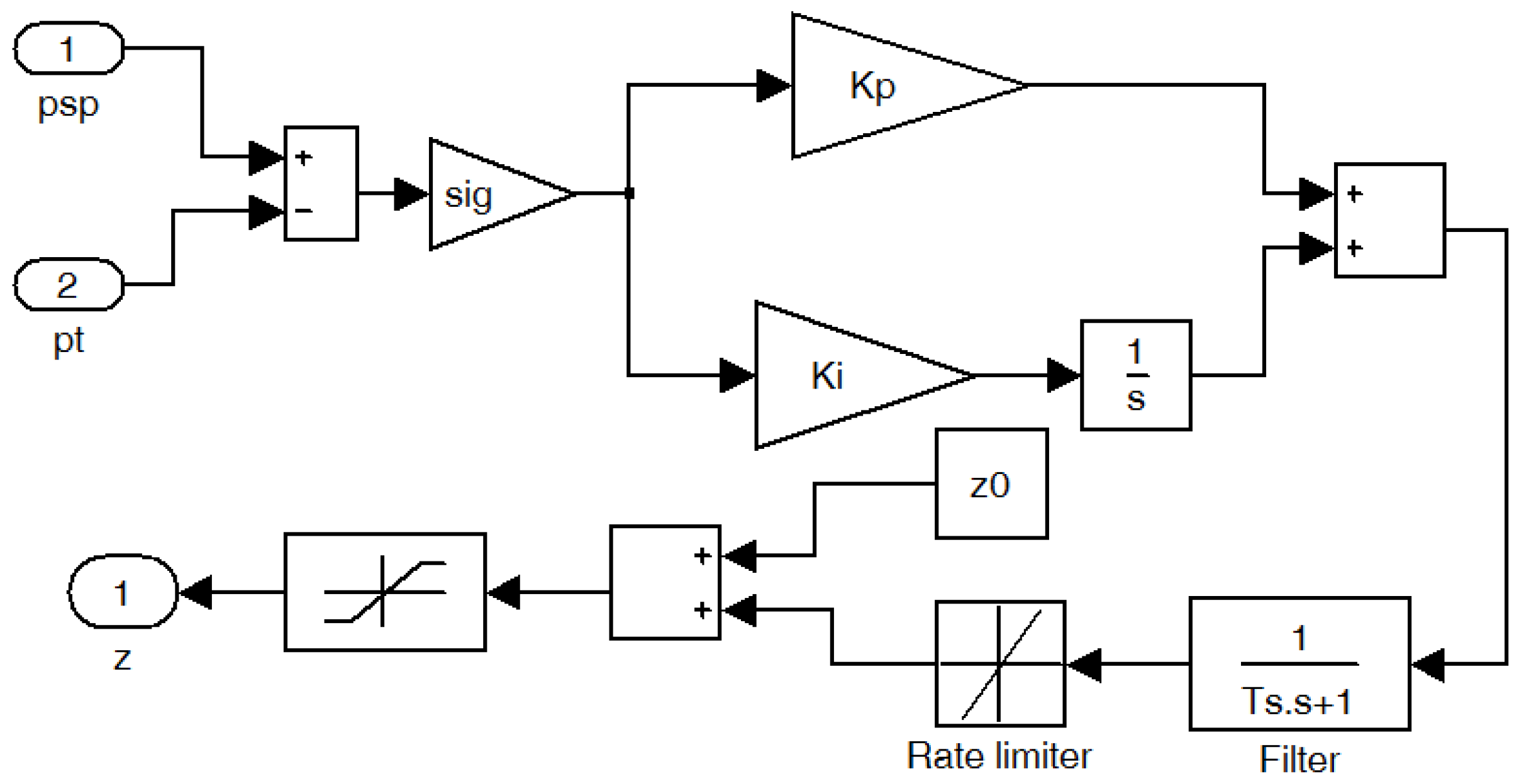
Once the worst likely sequences (WLS) were identified, the following step was to devise how to guarantee that the WLS will not make the STWL descend below the MSL, by acting either on the AGC signal or the turbine governor gains. Regarding the turbine governor, different governor settings (i.e., different combinations of K_p and K_i) were tested. For the sake of clarity, only three different settings are considered in the paper; the authors believe that it suffices to illustrate the problem presented here. The extension of the analysis to other governor settings is straightforward. The settings used in the paper are the ones implemented in the power plant before the runner replacement (present) and those proposed in [17] (Hovey) and [29] (Kundur). K_p and K_i values corresponding to each of these settings are included in Table 2.

Table 2. Governor gains used in the paper.

Governor gains	Present	Hovey	Kundur
Kp	2.8571	2.3795	2.1050
Ki	0.9524	0.4719	0.3429

Table 2. Governor gains used in the paper.

Governor gains	Present	Hovey	Kundur
Kp	2.8571	2.3795	2.1050
Ki	0.9524	0.4719	0.3429

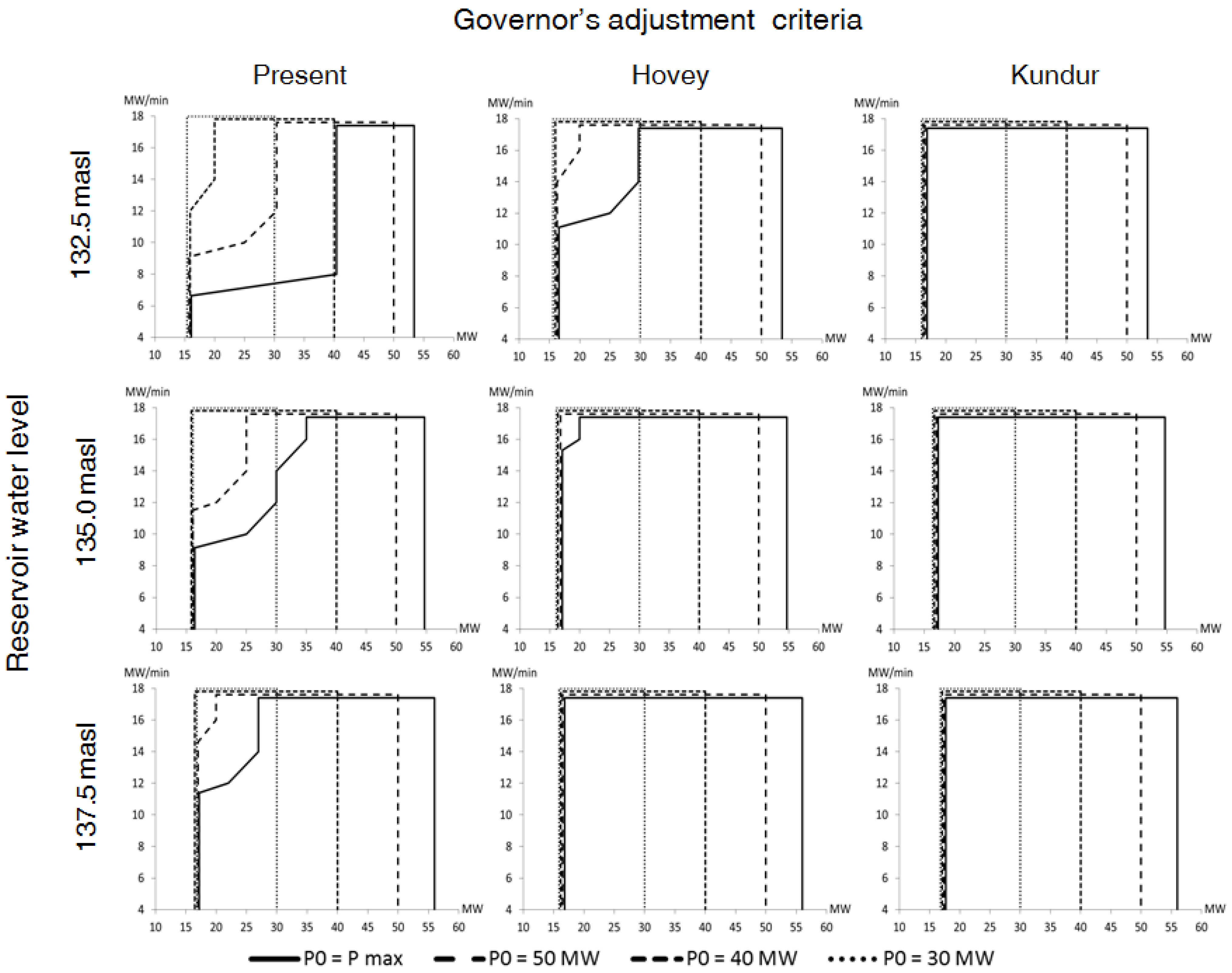
Regarding the AGC signal, a state-dependent rate limiter is proposed. From the previous discussions, it is obvious that for given governor settings, the WLS are different as a function of the initial operating condition; hence the use of a state-dependent rate limiter. On the one hand, the higher the reservoir level, the lower the probability that the STWL descends below the MSL, and consistently, a less severe rate limit can be used. On the other hand, under the above-mentioned assumption, the bigger the initial output power, the wider the power regulation range and the higher the probability that the STWL descends below the MSL, so more severe ramp limits should be used. In order to determine the state-dependent ramp limit, several simulations were carried out for each turbine governor setting, with different initial reservoir levels, output power, RS and RD. The results of these simulations corresponding to the three different reservoir levels are summarized in Figure 11.

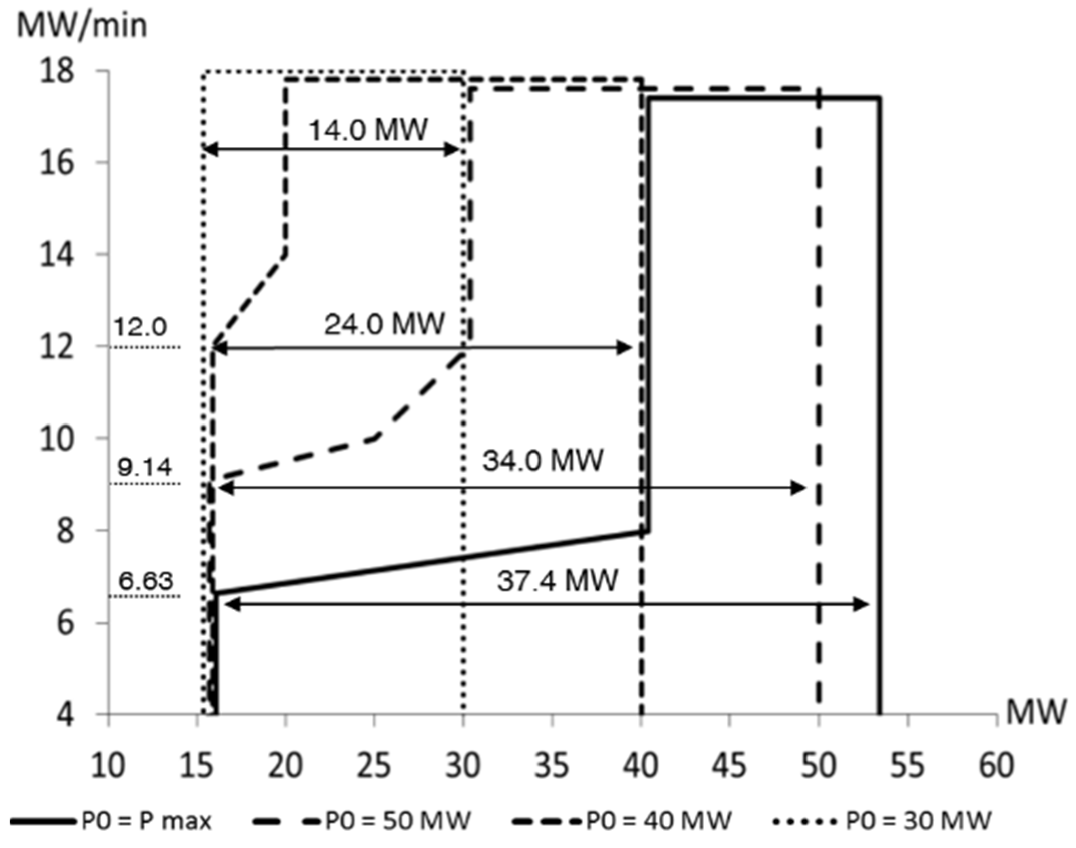
In order to better understand Figure 11, the graph corresponding to the present settings and an initial reservoir level of 132.5 masl (upper left graph) has been depicted with a higher level of detail in Figure 12. The area enclosed within the solid line gives the relation between the ramp limit and magnitude, for an initial output power of 53.4 MW (maximum output power corresponding to the above-mentioned reservoir level); ramp magnitude may be understood as the power band that could be offered for secondary LFC. For example, for a ramp magnitude or power band equivalent to the entire feasible power regulation range (37.4 MW), the ramp limit should be lower than or equal to 6.63 MW/min or, alternatively, should the power plant operator want to provide secondary LFC with the maximum ramp limit (18 MW/min), corresponding to the maximum technically feasible wicket gate opening rate, the offered power band should not exceed 13.4 MW. It should be noted that for the sake of clarity, both in Figure 11 and Figure 12, the “regions” corresponding to different initial output powers are slightly displaced from each other.

Figure 11. Ramp limits or maximum power bands for secondary load-frequency control (LFC), for different initial reservoir levels (132.5, 135, 137.5 masl), initial output powers (P0) and governor settings (Present, Hovey, Kundur).

Figure 11. Ramp limits or maximum power bands for secondary load-frequency control (LFC), for different initial reservoir levels (132.5, 135, 137.5 masl), initial output powers (P0) and governor settings (Present, Hovey, Kundur).

Figure 12. Ramp limits or maximum power bands for secondary LFC, for an initial reservoir level of 132.5 masl, present governor settings and different initial output powers (P0).

Figure 12. Ramp limits or maximum power bands for secondary LFC, for an initial reservoir level of 132.5 masl, present governor settings and different initial output powers (P0).

As can be seen in Figure 11, present governor settings are more responsive to AGC signals than Hovey and Kundur ones, and therefore, ramp limits for given power band, initial reservoir level and output power are more severe for the present governor settings. In addition, Figure 11 shows that for given governor settings and initial output power, ramp limits are less severe as the initial reservoir level increases. For Kundur governor settings and initial reservoir levels of 132.5, 135 and 137.5 masl, the ramp limit corresponds to the maximum technically feasible wicket gate opening rate (MXGOR), regardless of the initial output power or power band.

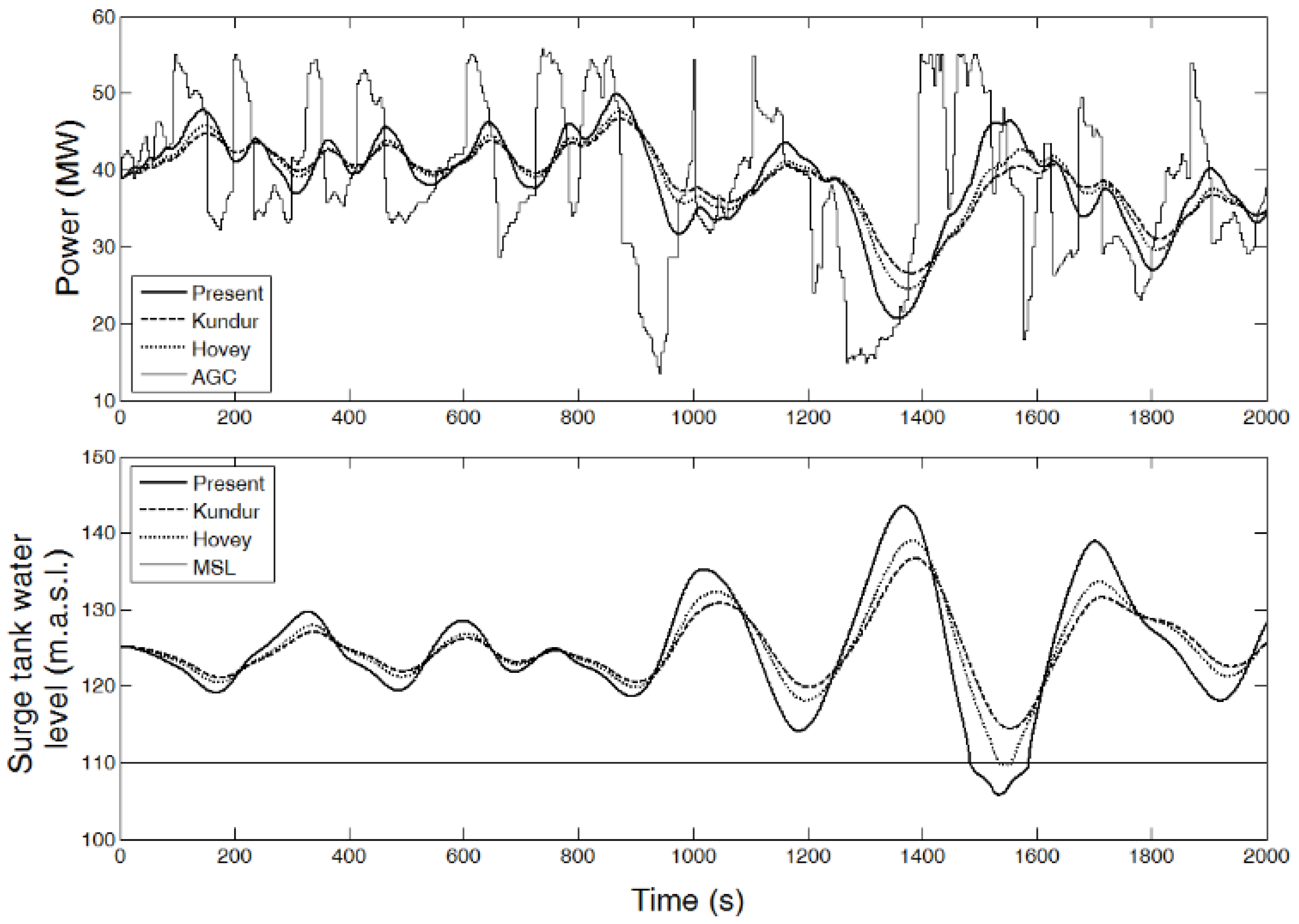
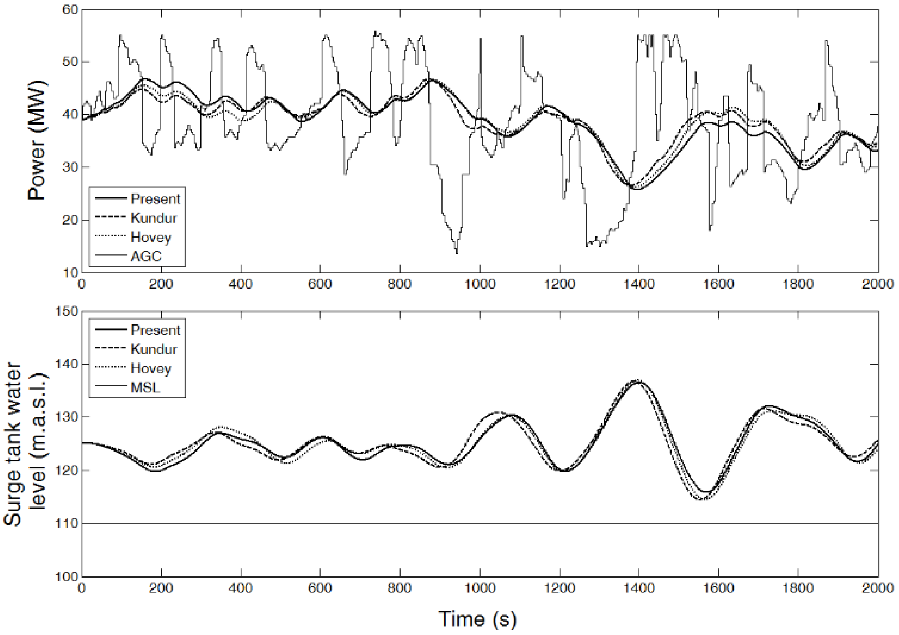
Finally, in order to check the validity of the proposed solutions and to compare them to each other, the response of the power plant to a set of 120 realistic AGC signals was simulated with and without considering the proposed ramp limit (PRL) for present and Hovey governor settings. In the cases where the PRL is not considered, MXGOR was used instead. In agreement with Figure 11, for Kundur governor settings, simulations were performed only with MXGOR. AGC signals were properly scaled according to the technically feasible power regulation range in all cases. The output power and STWL in response to one of the AGC signals, without and with the PRL, is presented in Figure 13 and Figure 14 for the three different governor settings. As can be seen in Figure 13, with present and Hovey governor settings, the STWL descends below the MSL when the PRL is not implemented. From the comparison between Figure 13 and Figure 14, it can be stated that in this case, the PRL effectively prevents the STWL from descending below the MSL.

Figure 13. Output power and surge tank water level in response to an AGC signal for different governor settings (Present, Hovey, Kundur), with the maximum technically feasible wicket gate opening rate (MXGOR). AGC: automatic generation control.

Figure 13. Output power and surge tank water level in response to an AGC signal for different governor settings (Present, Hovey, Kundur), with the maximum technically feasible wicket gate opening rate (MXGOR). AGC: automatic generation control.

Figure 14. Output power and surge tank water level in response to an AGC signal for different governor settings (Present, Hovey, Kundur), with the proposed ramp limit (PRL).

Figure 14. Output power and surge tank water level in response to an AGC signal for different governor settings (Present, Hovey, Kundur), with the proposed ramp limit (PRL).

Simulation results are summarized in Table 3, where N_nc is the average percentage of cycles during a simulation in which the plant fails to comply with the response criteria proposed in [30] (referred to as response quality), and S is the total number of simulations in which the STWL descends below the MSL (as a consequence of which the unit would trip). Simulations results are wholly consistent with the regions presented in Figure 11. According to Table 3, there was no simulation in which the STWL descended below the MSL with Kundur governor settings, just as predicted in Figure 11. Furthermore, in agreement with Figure 11, the number of simulations in which the STWL descended below the MSL was greater for present governor settings than for Hovey ones (120 vs. 24). These results supports the validity of the assumptions made to determine the WLS of AGC signals. In addition, as can be seen in Table 3, for present and Hovey governor settings, the STWL descended below the MSL in 120 (100%) and 24 (20%) simulations, respectively, when MXGOR was used as the ramp limit, whereas when the PRL was applied, the drawdown of the surge tank did not occur anymore, which demonstrates the effectiveness of the PRL to prevent the STWL from descending below the MSL and supports the soundness of the methodology proposed to determine the PRL. Of course, the implementation of the PRL comes at the expense of the response quality. As can be seen in Table 3, the response quality corresponding to present and Hovey governor settings worsened significantly as a result of the PRL implementation. With Kundur settings, it does make sense to talk about the effects of the PRL implementation on the response quality, since according to Figure 11, it is not necessary to implement any ramp limit different from the MXGOR. However, it is interesting to note that the response quality obtained for Kundur governor settings is, respectively, 18% and 97% worse than that obtained for Hovey and present settings when MXGOR is used as ramp limit. Of course, the final decision on the governor settings and ramp limit is to be made by the power plant operator and will depend on its degree of risk-aversion and on the economic penalty, if any, imposed by the Transmission System Operator (TSO) for both the violation of the LFR quality requirements and the non-fulfillment of the power reserve schedule that could occur as a consequence of the surge tank drawdown. The methodology presented in this paper is intended to be of help for the power plant operator to make these decisions.

Table 3. Average percentage of cycles in which the power plant does not comply with the response criteria.

Ramp limit	Present		Hovey		Kundur
-	Nnc (%)	S	Nnc (%)	S	Nnc (%)	S
MXGOR	2.631	120	4.398	24	5.191	0
PRL	8.634	0	7.404	0

Table 3. Average percentage of cycles in which the power plant does not comply with the response criteria.

Ramp limit	Present		Hovey		Kundur
-	Nnc (%)	S	Nnc (%)	S	Nnc (%)	S
MXGOR	2.631	120	4.398	24	5.191	0
PRL	8.634	0	7.404	0

6. Conclusions

In this paper, a simulation model has been used to investigate the cause of several unexpected high amplitude oscillations that occurred in the STWL of a real hydropower plant during secondary LFC maneuvers, after the replacement of the turbine runner, as well as to propose solutions that allow the power plant to continue providing secondary LFC in an acceptable manner. The model has been calibrated from data gathered during a series of on-site tests.

The cause of the high amplitude oscillations turned out to be a sort of resonance phenomenon, which takes place when the power plant operates under the control of an AGC system, in response to some sequences of power set-point signals that meet certain conditions. After making some assumptions, the characteristics of the WLS of AGC signals were determined by means of simulations.

Two different solutions have been proposed in order to guarantee that the WLS will not provoke the surge tank drawdown. The first solution consists of using a state-dependent load change rate limiter, whose ramp limit values depend on the initial output power and reservoir volume. In order to determine the state-dependent ramp limits, the WLS are simulated for different initial output powers and reservoir levels. The second solution consists of modifying the turbine governor gains.

The proposed solutions were tested against a set of realistic AGC signals by means of simulations. Simulation results demonstrate the effectiveness of the state-dependent rate limiter to prevent the surge tank drawdown and support the soundness of the methodology proposed to determine the ramp limit values. Furthermore, simulation results clearly illustrate the trade-off between the quality of the secondary LFC and the probability of occurrence of the surge tank drawdown. Even though the state-dependent rate limiter manages to prevent the surge tank drawdown, it comes at the expense of the quality of the secondary LFC response.

The methodology presented in the paper can be of use to both determine a feasible capacity expansion in the pre-planning phase of a hydropower plant upgrade project and to make decisions on the most suitable solution to be adopted after the execution of the upgrading works of a hydropower plant.