Review

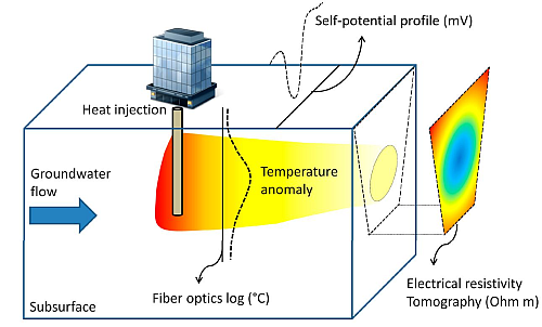
Geophysical Methods for Monitoring Temperature Changes in Shallow Low Enthalpy Geothermal Systems

1
Applied Geophysics, University of Liege, Chemin des Chevreuils 1, 4000 Liege, Belgium
2
Department, AQUALE SPRL, Rue Montellier 22, 5380 Noville-les-Bois, Belgium
3
Department of Geophysics, Colorado School of Mines, Golden, CO 80401, USA
4
ISTerre (Institut des Sciences de la Terre), CNRS, UMR CNRS 5275 (Centre National de la Recherche Scientifique), Université de Savoie, 73376 Cedex, Le Bourget du Lac, France
5
FNRS (Fonds de la Recherche Scientifique), 1000 Bruxelles, Belgium
*
Author to whom correspondence should be addressed.
Energies 2014, 7(8), 5083-5118; https://doi.org/10.3390/en7085083
Submission received: 15 May 2014 / Revised: 15 July 2014 / Accepted: 22 July 2014 / Published: 11 August 2014
(This article belongs to the Special Issue Geothermal Energy: Delivering on the Global Potential)

Abstract

:
Low enthalpy geothermal systems exploited with ground source heat pumps or groundwater heat pumps present many advantages within the context of sustainable energy use. Designing, monitoring and controlling such systems requires the measurement of spatially distributed temperature fields and the knowledge of the parameters governing groundwater flow (permeability and specific storage) and heat transport (thermal conductivity and volumetric thermal capacity). Such data are often scarce or not available. In recent years, the ability of electrical resistivity tomography (ERT), self-potential method (SP) and distributed temperature sensing (DTS) to monitor spatially and temporally temperature changes in the subsurface has been investigated. We review the recent advances in using these three methods for this type of shallow applications. A special focus is made regarding the petrophysical relationships and on underlying assumptions generally needed for a quantitative interpretation of these geophysical data. We show that those geophysical methods are mature to be used within the context of temperature monitoring and that a combination of them may be the best choice regarding control and validation issues.

Graphical Abstract

1. Introduction

Geothermal heat pumps have a lot of advantages over standard heating and/or cooling systems such as gas or oil boilers and cooling machines which render them sustainable [1,2]. They allow large primary energy savings (e.g., [3,4]), strong reductions of CO2 and other greenhouse gases emissions ([2,5] and references therein), and the use of energy stored in the subsurface (soil or groundwater). With regards to air-source heat pumps, geothermal heat pumps have the advantage of the ground temperature, which is far more constant than air temperatures. This energy is considered to be renewable as long as it is used reasonably and rationally (e.g., [6] and references therein). For instance, among shallow and deep geothermal resources, geothermal heat pumps accounted for 47.2% of thermal energy use and 68.3% of the total installed capacity in the World in 2010 [7]. Geothermal energy resources therefore constitute an essential field of research and development in the diversification of energy resources to hinder global warming (e.g., [8]).
Two main techniques exist to exploit shallow geothermal energy systems. In closed systems, heat is collected through a heat exchanger (vertical or horizontal), generally plastic pipes with a circulating fluid. This technology is generally referred as ground source heat pumps (GSHP). Such systems can be used for heating in winter and cooling in summer, suing the heat stored in the ground. Such a closed system is called borehole thermal energy storage (BTES). In open systems, groundwater circulates between production and injection wells and/or towards surface water. This is referred as groundwater heat pumps (GWHP) [9]. This kind of system requires a relatively high permeability to allow large pumping volumes. When heated or cooled water is infiltrated directly in the aquifer, one can take advantage of this energy storage as long as hydrogeological requirements are met (a weak hydraulic gradient for example). In this specific case, we rather speak of (seasonal) aquifer thermal energy storage (ATES) systems [4].
Very low-temperature systems (<30 °C) are generally located at depths between 0 and 100 m. They are thus much more easily accessible and involve lower implementation costs than deeper, high temperature, systems. The cost difference is essentially due to the drilling costs. Moreover, very low-temperature reservoirs, such as shallow aquifers, are relatively abundant in alluvial or coastal plains where urban development is concentrated. From 0 to less than 100 m depth, groundwater has an average temperature ranging from 5 to 30 °C and may be used for domestic or industrial cooling and/or heating (e.g., [10,11]).
Designing such systems requires a multidisciplinary approach including geological and hydrogeological studies. The most common approach is to model the subsurface using a coupled groundwater, heat flow and transport simulator. However, such models require the knowledge of the parameters governing groundwater flow (e.g., hydraulic conductivity and specific storage) and heat transport (e.g., thermal conductivity, volumetric heat capacity, flow rate). In situ tests, such as thermal response tests [12,13] or laboratory measurements [14] are sometimes possible, but the values obtained may deliver only well-centered information or may not always (if not at all) be representative of in situ conditions at a larger scale. Such data are often scarce if not missing and authors often have to rely on standard calculation charts, values found in the literature, or simply default values implemented in standard software (e.g., [15,16,17,18]). In addition, the heterogeneity of the material properties and their potential anisotropy, which are difficult to detect with standard integration methods, make the problem more complex. The direct consequence is a lower confidence in the predictions of models leading to inadequate design of the heat pumps.
Besides the characterization of shallow geothermal systems themselves (e.g., for dimensioning purposes), the impact on the evolution of groundwater temperatures is also an important research topic both economically and environmentally. From an environmental point of view, the exploitation of geothermal heat pumps yields cold and hot plumes [19,20,21] which may influence aquifer properties such as groundwater chemistry (e.g., [22,23,24]) and microbiology [25]. Moreover, geothermal systems can only be qualified as renewable if there is a global annual thermal equilibrium. These potential environmental effects must be (and will increasingly be) studied because they can have strong economic repercussions such as lowering the global life of the system with side effects such as aquifer freezing and scaling on heat exchangers and wells [6,26,27]. From an economical point of view, a better knowledge of the thermal affected zone (TAZ) [28,29] can prevent shallow geothermal systems competing with each other (thermal feedback or thermal recycling) [30,31] or better, to take benefit of multiple ATES systems with mutual energy storage zones to enhance the global systems efficiency [22].
Haehnlein et al. [6,11] pointed out that while policies exist in some countries to limit the temperature difference caused by the use of geothermal systems, the development of anomalies is rarely monitored. With the growth of the demand for renewable energy (more than 200 new ATES systems are currently being installed each year in The Netherlands, for example) [22], we can expect that regulations will become more severe and control of installations more common. New monitoring technologies will therefore be needed to better conceptualize, design, and then control shallow operating geothermal systems.
Thermal tracing experiments have been performed for decades in hydrogeology [32,33,34]. Such experiments are used to improve the characterization of hydrogeological parameters (e.g., hydraulic conductivity and hydrodynamic dispersivity tensors), but the same methodologies may also be used to study the thermal properties of shallow geothermal systems [35,36,37]. However, the heterogeneity of geothermal and hydrogeological systems may be too complex to be fully captured by classic thermal or solute tracer experiments alone [38,39], with only punctual measurements in wells.
In this context, new technologies are clearly needed to monitor the spatial and temporal distributions of temperature in the shallow geothermal system (Figure 1) to: (1) better design the geothermal system and the monitoring network, (2) prevent any thermal feedback/recycling, and (3) image and control the thermal affected zone. Among these technologies, we will emphasize in our review three emerging geophysical techniques to monitor geothermal systems (Figure 1). The first one is called electrical resistivity tomography (ERT) or electrical resistivity imaging (ERI). It provides 2D or 3D tomograms of the resistivity distributions of the subsurface. Time-lapse variations of the electrical resistivity can be used to map changes in temperature. The second approach is the self-potential method (SP), which is used to map or monitor the electrical potential at the ground surface or in wells. The self-potential anomalies can be associated with ground water flow and temperature variations. The last method is the use ofan in situ fiber optic distributed temperature sensor (DTS). This method provides linear measurements of temperature with centimeter resolution in boreholes with a precision of around 0.1 °C.
Figure 1. Emerging geophysical technologies to measure the temperature distribution in the subsurface due to heat injection in a fully non-invasive manner (electrical tomography and self-potential) to spatially continuous measures in boreholes (distributed fiber optics).
Energies 07 05083 g001
The paper is organized as follows: first, we describe the principles of the three methods with a focus on the information provided in the framework of geothermal systems, hypothesis made and set up. Then, a review of the literature for the three methods with emphasis on practical consideration and limitations is made. The paper ends with conclusions, perspectives of development and applications of these methods to geothermal heat pump systems.

2. Electrical Resistivity Tomography
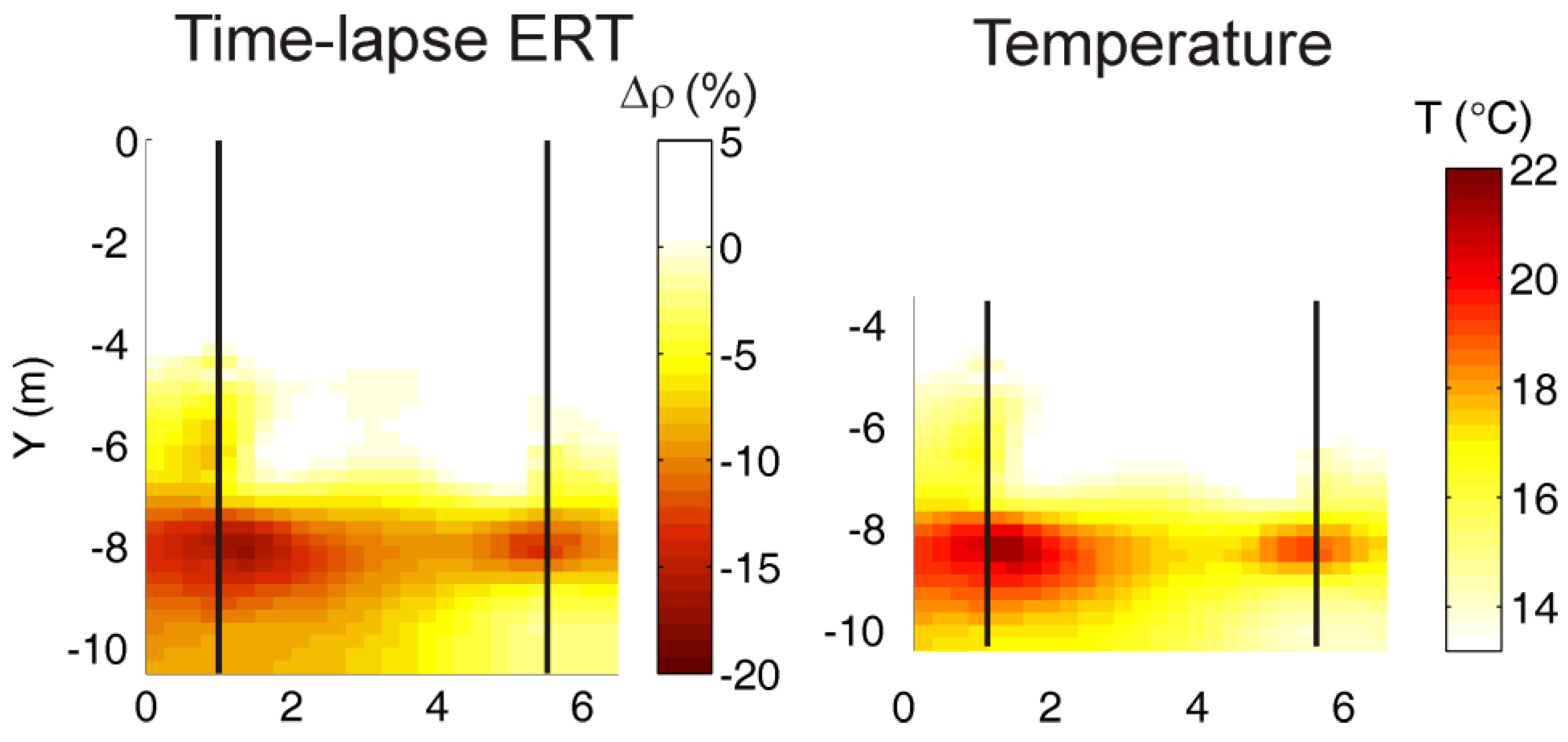
Electrical resistivity tomography (ERT) is a method that images the bulk electrical resistivity distribution of the subsurface (Figure 2) in two, three, or four dimensions (the three dimensions of space plus time when monitoring is performed) from the meter to the hundreds of meter scale depending on the electrode spacing. When conducted from the surface only, the method is non-invasive. Electrical resistivity is a property depending on several textural properties of the porous material (such as porosity and pore shape), the presence of clay minerals (mineralogy and weight fractions), the properties of the pore water (saturation, salinity), and environmental variables such as temperature [40,41,42]. As a consequence, ERT is often used to infer these subsurface properties but require being able to separate the different contributions affecting the measurements. Quantitative interpretation remains indeed difficult without additional information, generally in the form of a few additional in situ measurements or/and the use of additional geophysical methods (for instance GPR or induced polarization). Electrical resistivity tomography (ERT) has proven its efficiency to image and/or monitor spatial phenomena [43] such as salt water intrusions [44,45], variations in moisture content (e.g., [46,47]), biodegradation of hydrocarbons (e.g., [48,49]) and salt tracer experiments (e.g., [50,51] and references therein). An in-depth review of electrical properties of rocks can be found in Schön [52] or Revil et al. [53], whereas a description of electrical methods can be found in Binley and Kemna [54].
Figure 2. Background tomography obtained using 28 electrodes in two boreholes. The inverse model shows resistivity values varying between 100 and 200 Ω·m. The panel seems slightly heterogeneous and reflects lithological changes. Dots show the position of borehole electrodes. Average groundwater temperature is around 13 °C (modified after [55]).
Energies 07 05083 g002
The tomography of Figure 2 shows a background snapshot of the resistivity distribution at a site in an alluvial plain [55]. The changes in resistivity reflect changes in the lithology. To obtain such an image, a series of electrical current injections into the soil was performed, generally between two electrodes called current electrodes and the resulting electrical potential difference was measured simultaneously between two other electrodes, called potential electrodes. Given Ohm’s law, the ratio between the measured difference of electrical potentials and the known current intensity equals the electrical resistance. A value of electrical resistance is therefore assigned to the used quadrupole and the process is repeated automatically hundreds to thousands of time along a profile (or a panel for cross-borehole application) to acquire a full data set. Electrical resistance is not an intrinsic property of earth because it is linked to the volume of subsurface that is scanned by electrical current lines. The resistance data set must be inverted to find an inverse model of electrical resistivity distribution that explains collected data. This inverse model is the electrical image/tomogram that is then interpreted physically in terms of temperature using a petrophysical transformation (see Section 2.2). A common way to solve such inverse problems [54] is to add a regularization constraint to the least-square problem [56]. The problem is then to minimize, through an iterative process, an objective function of the form:
ψ ( m ) = ψ d ( d , m ) + λψ m ( m , m 0 )
In the above equation, m represents the (unknown) model vector (i.e., a vector containing the resistivity values for the cells used to discretize the subsurface), ψd(d,m) is a measure of the data misfit (difference between the measured and modeled data according to a given norm), the model functional ψm(m,m0) defines desired model constraints and can include a prior resistivity model m0, and λ is the so-called regularization parameter, which balances the two terms. This regularization parameter can also be optimized in the inversion process. Minimizing the objective function with respect to the model vector m is a non-linear problem in ERT. The solution of this problem can be achieved using an iterative process such as the Gauss-Newton algorithm.

2.1. Time-Lapse ERT

Bulk electrical resistivity of saturated soil/rock samples decreases with temperature [40,41,57]. This correlation reflects the change in conductivity of water contained in the pores but also in the surface conductivity of grains. These effects are linked to the modification of viscosity with temperature which modifies the mobility of charge carriers. By extension, the temperature changes observed on operating GWHP/ATES systems [4] are typically in the range of temperature changes that could be detected by ERT (~2 °C and more, see [55]).
During a monitoring study, we acquire at least one snapshot, which is linked to a background or reference state, such as the one shown in Figure 2. Data acquisition is then repeated over time with the same sequences, parameters and so on. Data sets are finally inverted and compared to the reference image to visualize resistivity changes over time. These changes are in turn connected to the physical process we want to follow (temperature changes in our case, Figure 3). One advantage of such time-lapse ERT over static ERT is that it can be used to monitor processes involving only one or a few of the parameters influencing electrical resistivity. This makes the interpretation of time-lapse ERT more easily quantitative.
In most monitoring studies, temperature effects are undesirable and therefore, often considered as noise that may create artefacts and misinterpretation of the resulting images. As a result, temperature corrections in time-lapse (monitoring) series may be necessary to correct electrical resistivity tomography results in order to avoid misinterpretation when explaining resistivity changes linked to other physical processes such as changes in contamination or porosity [40,58,59,60].
With time-lapse data sets, we are interested in imaging the changes in electrical conductivity/resistivity with respect to a reference in time. Generally, the process of inversion is adapted in order to improve inversion results [61]. Three main procedures, with several variants, exist to invert for time-lapse ERT data [62]: namely independent inversion, difference inversion, and time-constrained or reference model inversion.
In independent inversion, inversion results obtained separately are simply subtracted [63], which should eliminate systematic errors but amplify uncertainties in the data. The difference inversion scheme [50,64] formulates the problem in terms of variations for both data and model, i.e., the data differences are inverted to calculate the model changes to apply to the reference state. This process eliminates the systematic errors on the data linked to modeling, measuring device or contact resistances. The background state is used as a starting model for subsequent time-lapse, which generally leads to a fast convergence of the algorithm.
Figure 3. Tomographies of changes in bulk electrical resistivity after injecting hot water (3 m3/h at a mean temperature of 38 °C). The background tomography is the one shown in Figure 2. Hot water injected in a well located at 8m upgradient, on the whole aquifer thickness, can be seen as negative resistivity changes (blue). It is preferentially found in the deeper part of the aquifer because groundwater flows preferentially in this high hydraulic conductivity zone (gravel). This figure compares time-lapse inversions using the standard smoothness constraint regularization (left), minimum gradient support (middle) and geostatistical inversion (right) (modified after [65]).
Energies 07 05083 g003
For temporally constrained schemes, a regularization operator is added in the time dimension (under the form of a reference model) in addition to the space dimensions, to minimize changes between successive tomograms [66,67]. This provides a 4D inversion scheme, which has proven to be efficient in tracer tests [68].
According to the location of electrodes on the field, the inversion is made using a true 3D model. The subsurface is divided in cells in the three dimensions and the model is inverted considering current flow in all directions [69]. When the collected data results from electrodes situated on a plane, the inversion generally uses a 2.5D scheme, where the resistivity distribution is considered as constant in the direction perpendicular to the section [70]. The latter inversion scheme may yield inversion artefacts when used in time-lapse mode. Indeed, in the case of a moving plume of heat, it may be imaged before crossing the ERT section because it already influences current lines. This phenomenon is known as the shadow effect [71,72].
To compare the successive models in the monitoring study, it is important that all data sets be inverted with the same level of data misfit corresponding to the expected noise level and the same approach to optimize the regularization parameter of Equation (1). Indeed, over-fitting the data may create artefacts of inversion in the corresponding image, whereas the contrary would result in an over-smoothed inverted section [73]. Similarly, using different approaches to optimize the regularization parameter (L-curve, fixed, iteratively decreasing) may introduce undesired artifacts.
Another issue is the assessment of the propagation of noise in the inversion. Robert et al. [51] proposed the use of two background data sets corresponding to a common state of the subsurface to study this phenomenon. They inverted one data set with the inversion of the other as reference. The resulting changes in resistivity are small and the maximum change is considered as the limit to interpret resistivity change. Hermans et al. [74] estimated the level of noise with reciprocal measurements and generated 100 new data background data sets. Then, they evaluated the mean and standard deviation of the 100 inverted electrical resistivity models and proposed a conservative cut-off (two times the maximum standard deviation) to interpret time-lapse images. Hermans et al. [55] used a simple physical interpretation to assess the error level. They expected only decreases in resistivity in their time-lapse sections. However, increases up to 3% were observed. They thus considered the changes between −3% and +3% has not interpretable and chose −3% as the limit of quantification for ERT in their specific case. This corresponded to a change in temperatures of 1.2 °C.
A major drawback of traditional ERT inversion is the smoothing effect induced by the regularization operator. To avoid this, coupled hydrogeophysical inversions are possible [39,75,76]. Resistance data are directly incorporated in the inversion of (thermo-) hydrogeological data, which avoids the inversion steps. Besides, many efforts have been made in the last decade to improve static ERT inversion by incorporating prior information in the inversion process. New constraints have been developed including blocky inversion [77], minimum gradient support [78], structural inversion [79], geostatistical inversion [44] or guiding images [80]. These constraints have proved to be efficient in many field cases (e.g., [81]).
Except for the reference model constraint used in the spatio-temporal and difference inversion scheme, few specific regularization operators have been developed for time-lapse ERT inversion. Globally, the same constraints as for static image could be used. Nguyen et al. [65] proposed to adapt minimum gradient support (MGS) and geostatistical inversions for time-lapse inversion. Figure 3 proposes a comparison of these approaches with standard smoothness constraint within the context of difference inversion. The models were inverted with the same error level to the same inversion error. Data correspond to the heat tracing experiments performed by Hermans et al. [55] in an alluvial aquifer with cross-borehole ERT. Hot water was injected in a well located 8 m upgradient on the whole thickness of the aquifer. The results obtained with the standard smoothness constraint (Figure 3, left) showed a good agreement with direct and DTS measurements. Hot water flows preferentially in the deeper part of the aquifer (gravel) due to its higher hydraulic conductivity. In this case, MGS yields focused resistivity changes and avoid smoothing (Figure 3, middle), which is efficient to image transport in fractures, karsts or along faults, but not really appropriate in an alluvial aquifer where flow is supposed to be relatively homogeneous. Geostatistical inversion in time-lapse allows integrating direct measurements in boreholes, such has DTS temperature logs, to build the regularization operator (Figure 3, right). Since, spatio-temporal variograms are possible [82], this could be included in a 4D inversion scheme as well. The geostatistical inversion reduces the smoothing effect of standard inversion to the suggested correlation length and is the most coherent with observed temperatures.
Qualitatively, the three inversions proposed in Figure 3 are similar. They enable to locate the zone of preferential flow path, related with stronger decrease of resistivity [55]. However, quantitatively, the variations in resistivity are slightly different which would in turn modify the estimation of temperature. It is thus important to consider the regularization operator which best fits the flow process. Direct measurements are helpful in this process. Even if those issues (noise and inversion) are not specific to the monitoring of temperature, they may play an important role in the future in the development of time-lapse ERT, and may thus influence its use within the context of geothermal systems.

2.2. Petrophysical Considerations

In the framework of ERT, the aim of the petrophysical relationship is to quantify the link between bulk electrical conductivity and temperature. The bulk electrical conductivity σb is generally expressed as a function of porosity ϕ and tortuosity (often joined in a term called the formation factor F), saturation Sw, fluid electrical conductivity σf and surface conductivity σs due to electrical conduction in the electrical double layer coating the surface of the grains in contact with water [83]:
σ b = 1 F S w n σ f + 1 F ϕ S w n 1 σ s
where n, the saturation exponent, is an empirical exponent close to 2. Surface conductivity is related to the cation exchange capacity of the matrix and is significant for shaly and clayey sediments. Description of experimental models investigating this term can be found in Waxman and Smits [42] or Revil et al. [41,84]. Archie’s law (Equation (3)) describes the relationship between F and the connected porosity ϕ with a power law through the porosity-exponent m [85]:
1 F = ϕ m
The formation factor F may vary spatially (both laterally and with depth), depending on the lithology. Revil [83] showed that it may be reasonable to take m = n. In this case Equations (2) and (3) becomes:
σ b = θ m σ f + θ m 1 σ s
where θ is the water content. Revil [83] showed that the surface conductivity can be related to the cation exchange capacity or the specific surface area of the material. Both parameters can be easily measured in the laboratory for core samples. Surface conductivity can also be determined through induced polarization measurements, which can be measured with the same instrument used to do resistivity measurements [86].
In saturated conditions (Sw = 1), Equation (2) simplifies to:
σ b = σ f F + σ s F ϕ
When surface conductivity is negligible, bulk electrical conductivity is directly proportional to fluid electrical conductivity:
σ b = σ f F
When limited temperature intervals are considered (a few tens of degrees), a linear dependence between water electrical conductivity and temperature can be assumed, it is called the ratio model. Equation (7) expresses the linear relation around a temperature of reference Tref [40,87]:
σ f , T σ f , T r e f = m f , T r e f ( T T r e f ) + 1
where σf,T is the fluid electrical conductivity at temperature T (in °C), σf,Tref is the fluid electrical resistivity at the temperature of reference Tref (typically 25 °C), and mf,Tref is the linear temperature dependence of electrical conductivity with temperature (expressed in °C−1). Equation (7) corresponds to a first-order Taylor expansion of the conductivity dependence with temperature around the reference temperature. The value of mf,25 can be experimentally determined and varies according to the composition of the fluid. A value between 0.018 °C−1 and 0.025 °C−1 is often found [40].
Surface conductivity variations with temperature can be expressed by similar equations, with a different fractional change per degree Celsius ms,Tref (°C−1):
σ s , T σ s , T r e f = m s , T r e f ( T T r e f ) + 1
Hayley et al. [40] applied this model on the temperature range 0–25 °C and found ms,25 around 0.018 °C−1 and mf,25 equal to 0.0187 °C−1. These values are similar and lead globally to a linear temperature dependence for the bulk electrical conductivity. It signifies that Equation (7) is also valid for bulk electrical conductivity which varies linearly with temperature. This is generally acceptable for temperature intervals below 40 °C but may be wrong for higher temperature intervals [41].
In the case of ERT monitoring studies, we measure bulk electrical resistivity at different time steps and compare it to a reference state, called the background. If we take the ratio of Equation (5) between a specific time-step (state 2) and the reference background (state 1), we have:
σ b 1 σ b 2 = σ f 1 + σ s 1 ϕ σ f 2 + σ s 1 ϕ
and the relation is not dependent on the formation factor but on porosity only. This can be done only if the formation factor is supposed to be independent from electrical conductivity and constant in time which is generally true. If surface conductivity can be neglected, Equation (9) simplifies further to:
σ b 1 σ b 2 = σ f 1 σ f 2
Through Equation (10), we see that the variation in bulk electrical conductivity in the saturated zone is related only to a variation of the fluid electrical conductivity. When we consider temperature variations, Equation (10) is also valid when surface conductivity is non-negligible if the temperature linear dependence of water and surface conductivity are the same [41]. Indeed, in this case the variations of water, surface and bulk electrical conductivity have the same slope, which allows writing Equation (10) as well.
Equation (10) may be interesting to use to derive subsurface temperature from water conductivity. Indeed, in many cases, temperature measurements will be only accessible through groundwater inside boreholes and the fractional change per degree will be determined from a water sample. In Equation (10), σb1 and σb2 are determined using ERT after inversion of resistance data and σf1 can be measured on a sample from formation water of the aquifer before the experiment (calibration process). The only unknown in Equation (10) is thus the fluid electrical conductivity at state 2 σf2, which can be expressed as:
σ f 2 = σ b 2 σ b 1 σ f 1
If we assume that the salinity of the fluid remains constant during the experiment, the water electrical conductivity depends only on temperature.
Introducing Equation (7) into Equation (11), we can express the temperature T (in °C) according to bulk electrical conductivity of the background and of the considered time-lapse section, to water electrical conductivity at the temperature of reference and at the temperature of the background and to the fractional change per degree Celsius:
T = 1 m f , 25 [ σ b 2 , T σ b 1 σ f 1 σ f , 25 1 ] + T 0
where σb2,T represents the bulk electrical conductivity at the time-step for which we try to determine the temperature and T0 = 25 °C.
In Equation (12), the ratio σ f 1 σ f , 25 is only dependent on the temperature and the fractional change per degree Celsius. We can thus deduce the absolute temperature in the aquifer according to the initial temperature T1:
T = σ b 2 , T σ b 1 ( T 1 T 0 ) + σ b 2 , T σ b 1 1 m f , 25 + T 0
Equation (13) is similar to Equation (7) expressed for the bulk electrical resistivity at two different temperatures. The result of applying these petrophysical relationships to changes in ERT can be seen in Figure 4.
The developments above consider that changes in bulk electrical conductivity are only related to direct temperature changes. It does not take into account modifications in equilibrium and kinetics that may arise with an increase in temperature.
Figure 4. Time-lapse tomography of changes in temperature derived from ERT using Equation (13) on Figure 3, left. The image of temperature is limited to the saturated zone, because Equation (5) is not valid in the unsaturated zone (modified after [55]).
Energies 07 05083 g004

3. Self-Potential Method

The self-potential method is a passive geophysical method that is sensitive to the generation of electrical current densities in the ground. The method consists in mapping or monitoring passively electrical potentials on the ground surface or in wells using a set of non-polarizing electrodes (e.g., Cu/CuSO4 or Pb/PbCl2 electrodes). One of these electrodes is used as a reference, preferably located far from the area that is being monitored. The instrument used for the measurement is a voltmeter with a sensitivity of at least 0.1 mV and an input impedance of 10 to 100 MΩ or higher.
These currents include, within the context of geothermal systems, the streaming current associated with the flow of the ground water and the thermoelectric current associated with a temperature gradient. The sum of these two terms corresponds to the total source current density j S :
j S = Q ^ V u + C T σ T
where u (in m·s−1) denotes the Darcy velocity, Q ^ V (in C·m−3) denotes the excess of electrical charge at saturation that is carried along with the flow of the pore water, σ denotes the (saturation-dependent) electrical conductivity of the porous material, and C T is the thermoelectric coupling coefficient defined below. For pH values between 5 and 8, Jardani et al. [88] found that the Q ^ V is controlled by the permeability at saturation k (in m2) and they developed the following empirical relationship [89]:
log 10 Q ^ V = 9.2 0.82 log 10 k
In conductive materials, the source current density j S is responsible for an electrical field and the tangential component of this electrical field is measured at the ground surface. With respect to the macroscopic electrical field, the generalized Ohm’s law for the total current density j (A·m−2) is written as:
j = σ E + j S
where E = φ denotes the electrical field and φ the self-potential field, and σ denotes the bulk electrical conductivity of the porous material. From Equations (14) and (16), the streaming potential and thermoelectric coupling coefficients Cs and CT are defined by:
C S = ( φ h ) j = 0 , T = 0
C T = ( φ T ) j = 0 , u = 0
and are expressed in V·m−1 and V·K−1 (or V·°C−1) respectively, where h is the piezometric level. In Equation (18), the thermoelectric coupling coefficient is only properly defined in absence of flow and when the total current density is zero. An experimental procedure is described in Leinov et al. [90]. In a recent work, Revil et al. [91] obtained a value of the thermoelectric coupling coefficient of −0.5 mV·°C−1. The negative polarity implies that positive temperature anomalies (increase in temperature) should be associated with negative self-potential anomalies.
Equation (16) is combined with a conservation equation for the electrical charge that is written as j = 0 in the quasi-static limit of the Maxwell equations [92]. The combination of these equations yields the following elliptic partial differential equation for the self-potential φ (in V):
( σ φ ) = j S
The right-hand side of Equation (19) corresponds to the self-potential source term associated with the Darcy velocity, with the temperature distributions, and with the heterogeneity in the distribution of the volumetric charge density, thermoelectric coupling coefficient, and electrical conductivity.
Figure 5 and Figure 6 show the simulation of the self-potential signals associated with the passage of an electrical potential anomaly in a preferential flow channel. We can see a negative self-potential anomaly at the ground surface indicating the presence of the thermal anomaly (Figure 5). This anomaly is highly correlated to the temperature changes (Figure 6).
Figure 5. Time-lapse simulation of electric potential in a tank, relative to the background, following the hot injection. 3D illustration of growth of the negative self-potential anomaly in the channel at the surface, due to the temperature distribution in the channel in the subsurface (modified after [93]).
Energies 07 05083 g005
Figure 6. Simulated temperature and electric potential changes relative to background along Profile 1 (see position in Figure 5) following the injection of hot water in an upstream reservoir. (a) Simulated temperature change relative to background. The temperature anomaly is confined primarily to the permeable channel; (b) Simulated electric potential change relative to background following the hot injection. The electric potential anomaly is negative, achieves a peak amplitude of approximately −13 mV, and is confined primarily to the permeable channel; (c) Simulated relationship between temperature change and electric potential change along profile 1. The relationship is linear and has a slope of −4.9 mV·K−1, which is approximately equivalent to the thermo-electric (intrinsic) coupling coefficient of CT = −5 mV·K−1 incorporated into the model, indicating the potential anomaly is due to the temperature change in the tank for this simulation (modified after [93]).
Energies 07 05083 g006

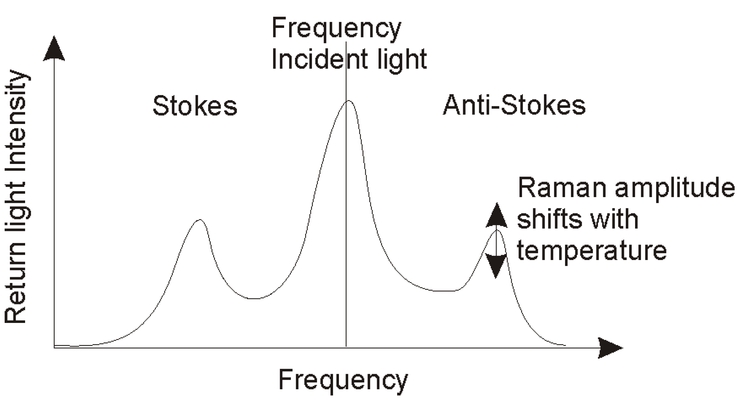
4. Distributed Temperature Sensing

Distributed temperature sensing is based on Raman scattering effect in fiber optic cables. Raman scattering is an inelastic scattering resulting from the interaction of an incident ray of light with the electrons in the molecular bond. Inelastic interaction means that the frequencies of incident and scattered photons are different (Figure 7). Frequency shifts correspond to the vibration frequencies of the electrons. Two states are possible: photons scattered to lower frequencies, corresponding to energy absorbed by the molecules, are called Stokes lines, whereas photons with higher frequencies, corresponding to a loss of energy from the molecules are called anti-Stokes lines. A detailed description of the effects can be found in Selker et al. [94].
Figure 7. Sketch of the Raman scattering effect in fiber-optic. Incident light is scattered due to the interaction of photons with electrons. The Anti-Stokes amplitude varies with temperature. Note that Brillouin scattering [94] has been ignored on the sketch.
Energies 07 05083 g007
The temperature dependence of Raman scattering is linked to frequency relations between incident and scattered photons. When temperature increases, the number of electrons in high energy states increases, too. Consequently, the ratio of anti-Stokes photons relative to Stokes photons will be higher. The ratio Rr of anti-Stokes to Stokes intensity in the back-scattered light is [95]:
R r = ( λ S λ A ) 4 exp ( h c Δ υ k T )
where λS and λA are Stokes and anti-Stokes wavelengths, c is the speed of light in vacuum, Δν is the frequency shift with incident light, h is the Planck’s constant, T is the absolute temperature (in Kelvin) and k is the Boltzman constant. This ratio is dependent on the temperature at the position corresponding to the two-way travel time only (it means that it is independent of light intensity). Practically, the diffusion of light and the measuring time result in an integrative rather than punctual measure of temperature. To achieve a high spatial resolution, the speed of light must be precisely known. Commercial fibers generally have a speed around 0.2 m/ns. It means that to 1 m of fiber corresponds 5 ns of signal to analyze with a delay of 10 ns/m for the backscattered signal to arrive (two-way travel time) at the measuring device. To avoid dispersion of light effects, the first and last parts of the signal are trimmed, leading to signal loss. This is a bigger issue for small spatial measuring interval, since the ratio trimmed signal over total signal is higher. The signal strength of Stokes and anti-Stokes photons is also a limit on the precision of the method. Longer integration times, averaging several pulses, will increase the number of photons and thus the resolution of the method (from around 0.1 °C down to 0.01 °C). The use of DTS to determine temperature will thus always be a compromise between, temperature precision, spatial and time resolutions.
Tyler et al. [96] provide guidelines for the use of DTS to measure temperature in hydrological studies. DTS allows achieving meter to centimeter resolution over long distances in 1D but requires the installation of boreholes. The measured temperature is that of the groundwater in open systems (Figure 8).
Figure 8. Comparaison of DTS and ERT-derived temperatures in borehole during heat tracing experiment (Figure 4). The agreement is very good which validates the ability of ERT. The difference in the upper part of the aquifer likely results from convection in the borehole. This effect is less important in ERT which provide a temperature on an integrated volume (modified after [55]).
Energies 07 05083 g008
Tyler et al. [96] also point out the importance of the calibration procedure to obtain accurate temperature data, taking into account signal attenuation (cables and connections dependent) and temperature offset (laser and sensor dependent). This is generally done using an ice bath at constant temperature (0 °C). Compared to thermocouples and traditional temperature loggers, DTS systems offer the advantage of providing distributed measurements of temperature using a single cable, making its implementation easier. If the measuring device is considerably more expensive in the case of the DTS relative to the thermocouple where a simple voltmeter is sufficient, the cost and installation of the DTS sensors is significantly lower per meter of installation.

5. Previous Works

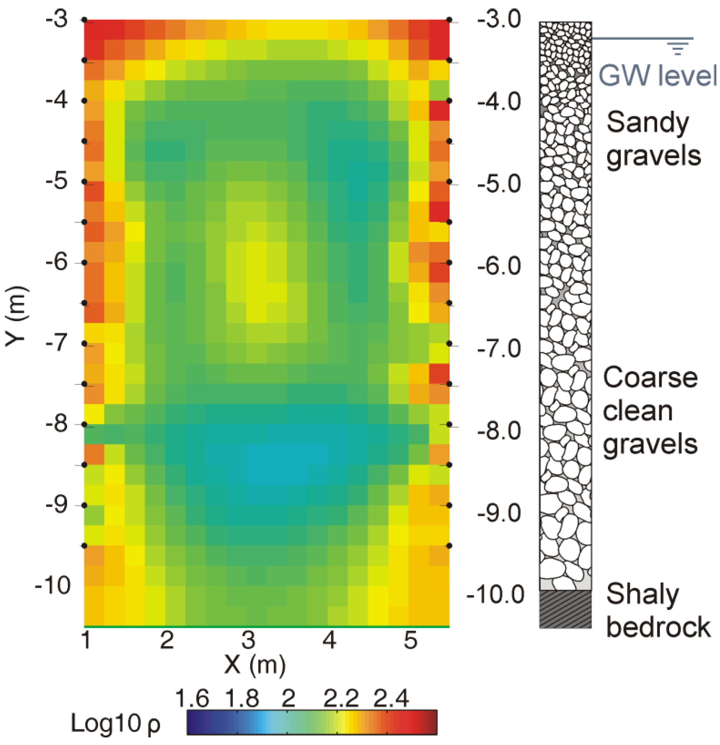
5.1. Using ERT to Monitor Temperature Changes

ERT has already been applied to study heat reservoirs where hydrothermal fluids generate high resistivity contrasts due to their temperature often exceeding 150 °C. In those situations, ERT can detect the reservoir itself, map preferential flow paths, and be useful to characterize rock properties [97,98,99,100]. Recently, several studies were carried out to image volcano hydrothermal systems with very long resistivity cables, showing that ERT is a reliable tool to detect hydrothermal features [101,102].
However, to our knowledge, few studies have used time-lapse ERT to estimate the temperature distribution during heat injection and storage experiment. The first geothermal test using geoelectrical methods was conducted by Benderitter and Tabbagh [103]. They carried out an experiment where the injection of heated water (40 °C) in a 4 to 7 m deep confined aquifer was monitored with DC resistivity measurements. The first potential electrode was fixed and used as a reference; the second one was covering the research area. At the time, the authors produced qualitative anomaly maps using percentage changes in electrical potential. These maps were interpreted using electrical forward modelling calculated for simple geometric subsurface models determined according to the injected volume and the expected temperature. They explained the existence of an electrical anomaly in bulk electrical resistivity (−33%) as the result from the injection of heated water (40 °C).
During the nineties, the development of automated acquisition systems resulted in a strong increase in the use of geoelectrical tomography methods in many contexts. Ramirez et al. [104] used cross-borehole time-lapse ERT to monitor a steam injection during a restoration process. Electrical resistivity being influenced by temperature and saturation effect, it was not possible to derive directly temperature from their measurements. Resistivity was initially expected to increase due to water displacement related to steam injection (decrease in saturation). However, a global decrease in resistivity was observed on the field. This change is explained by an increase in the conductance of exchange cations of clay minerals and increase in the ionic content of water. An US patent was even delivered for the application of the method for relatively high temperature variations in clayey soils [105].
LaBrecque et al. [106] monitored temperature changes within the context of Joule heating combined to vapour extraction during a remediation process with cross-borehole time-lapse ERT. They compared their results with temperature measurements but did not proceed to a conversion of ERT results into temperature. They analysed the variation in conductivity between background and time-lapse series in a partially saturated clay layer. During the first part of the monitoring, the mean temperature increased by 17 °C, and the corresponding conductivity change was coherent with expectations. Then, the temperature reached 100 °C and the change in conductivity was slightly smaller than expected by temperature effects only. It was explained by a decrease in saturation. At the end of heating, conductivity values were much below the background values showing an important loss of water produced by desaturation.
The two examples above show attempts to estimate the temperature effects on electrical resistivity in deposits dominated by clay, where the cation exchange capacity is responsible for the major part of electrical conductivity during strong heating procedure. At the opposite, Hermans et al. [74] went back to the idea developed by Benderitter and Tabbagh [103] to monitor changes in temperature related to the injection of heated water in aquifers. They successfully monitored with a surface profile the 3 days of injection of heated water (48 °C) at a relatively low rate (87 L/h) in a homogeneous sandy aquifer (10.5 °C, 2.5 m thick). Surface time-lapse ERT proved to be able to qualitatively follow such experiments by highlighting heat flow and diffusion around the well. Quantitatively, ERT-derived temperatures were similar to temperatures predicted by a thermo-hydrogeological model developed by Vandenbohede et al. [36]. However, a correction term accounting for the discrepancy between formation and injected (tap) water conductivity had to be calculated. This experiment proved that ERT also has a potential for temperature monitoring of clay-free sediments with low temperature variations. These conditions are typical of shallow open-loop geothermal systems.
Hermans et al. [55] extended this work for deeper and more complex reservoirs by implementing a new experiment in a heterogeneous sandy gravel alluvial aquifer (7 m thick). A heat injection (3 m3/h of formation water heated at 38 °C during 24 h) and pumping experiment (30 m3/h, 13 °C) was designed with a cross-borehole ERT panel crossing the main direction of flow. The ERT-derived temperatures in the panel (maximum change about 8 °C) were coherent with DTS temperatures and groundwater temperature loggers, allowing a spatially and temporally distributed quantitative estimation of temperature within the aquifer. ERT results, consolidated by an important amount of direct measurements, confirmed the heterogeneous nature of the aquifer (e.g., preferential flow paths). ERT proved its ability to detect temperature changes below 1.5 °C and then to follow lower incremental changes. The design of cross-borehole experiment allows more flexibility regarding the depth of the reservoir and the resolution since a major drawback of surface ERT is the loss of resolution/sensitivity with increasing depth [51,107].
Firmbach et al. [108] studied heat transport with ERT in an experimental box (1 m × 0.4 m × 0.4 m) with various levels of saturation. This experimental design enables to control temperature and heat fluxes within the box. The qualitative correlation between electrical resistivity and temperature was confirmed for two different media, but they did not provide a quantitative use of ERT to derive temperatures.
Qualitative and quantitative temperature monitoring have presently only been successfully attempted in favourable conditions (shallow aquifers) regarding the resolution/sensitivity of ERT and its depth of investigation. However, plenty of studies showed the ability of ERT in general to follow dynamic processes in less favourable conditions. As an example, Kemna et al. [50] and then Müller et al. [107] successfully used ERT in the Krauthausen test site in Germany to follow different types of tracer migration within a 10m thick heterogeneous and layered sandy aquifer. Supper et al. [109] demonstrated the ability of the method to study seasonal variations in permafrost. Auken et al. [110] showed the ability of 3D surface ERT to qualitatively detect changes in groundwater chemistry linked to the injection of CO2 (gas) in an aquifer to simulate CO2 leakage in the framework of CO2 geological storage. Firstly, the resistivity of groundwater decrease linked to the increasing water mineralisation caused by CO2 dissolution. Then, the resistivity started to increase when some scaling occurred (e.g., calcite). The authors confronted their 3D images with lots of ground truth data and showed that 3D time-lapse images reproduced well the affected areas.
Robert et al. [51] were able to qualitatively follow the injection of a salt solution in a fractured area in carboniferous limestone. With the help of two parallel surface ERT profiles, they managed to find the groundwater flow direction and the preferential flow paths at a depth of 20 m by taking great care during the experiment dimensioning and the data acquisition.
These studies present all the ability of non-invasive techniques such as ERT to follow dynamic processes occurring in aquifers with different geological conditions but also different depths that could be met during geothermal site prospection/characterization.

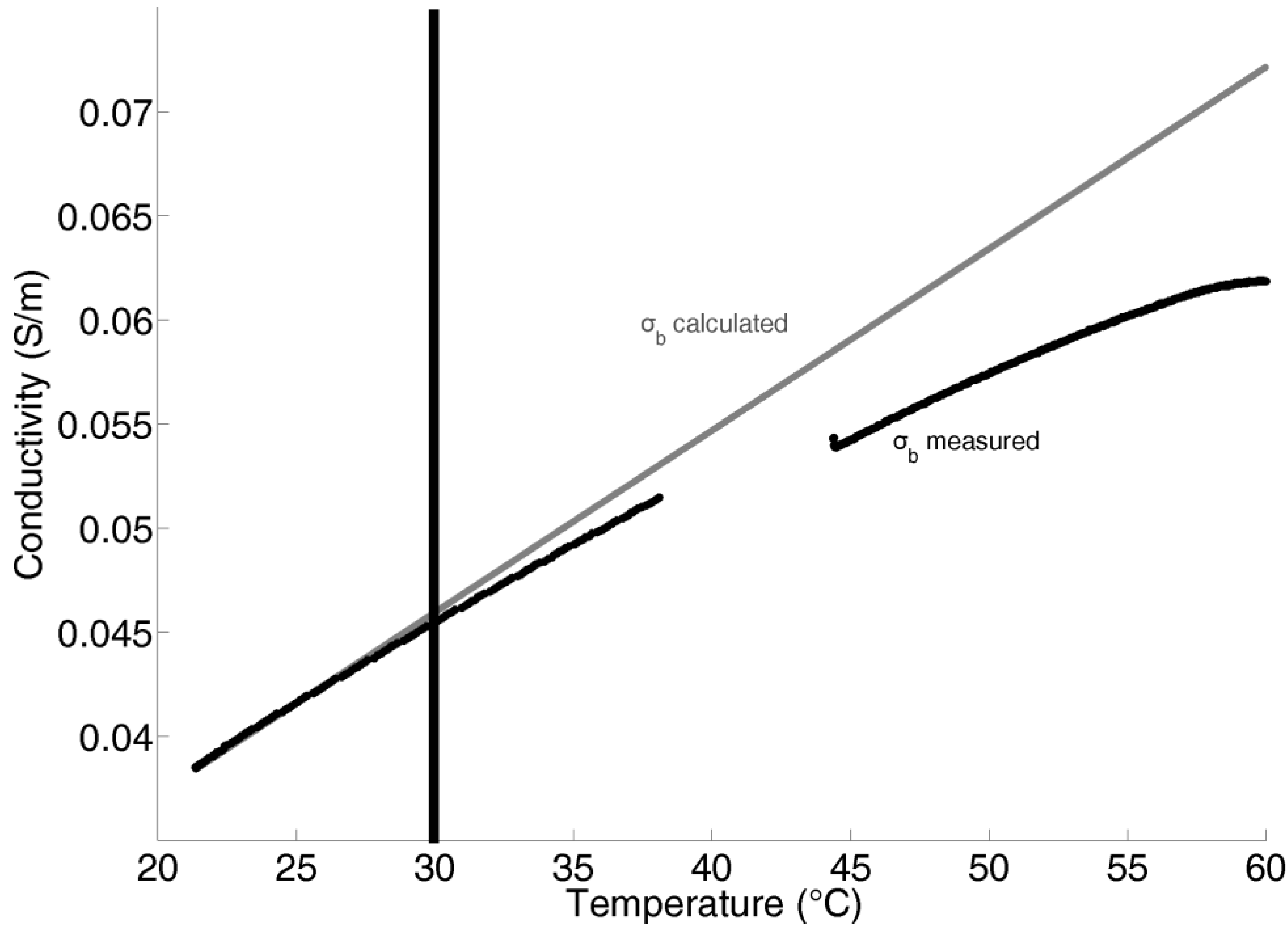
5.2. Petrophysical Considerations Regarding Electrical Conductivity

Equation (13) is the key to provide a quantitative estimation of temperatures using electrical resistivity temperatures. In addition to ERT measurements, it requires one to determine the fractional change per degree Celsius. A common practice is to collect a sample of formation water and to verify the linear relationship in the laboratory. The value of mf,25 is generally around 0.02. The representativeness of such a lab experiment may be questionable since the conditions are not representative of the subsurface systems. The test is sufficient to estimate the increase of electrical resistivity due to the viscosity effect. However, in presence of chemical and kinetics effects, the results may depend on the duration of the test (how quickly the temperature increases) and may neglect reactions occurring between the pore water and the solid matrix. These effects are not expected to be important for low temperature systems (<30 °C), at least for short experiments.
Another parameter to determine in Equation (13) is the initial temperature in the aquifer T1, in geothermal studies, such values will generally be available through direct measurements. Applying Equation (13) to a whole ERT section requires a few assumptions. First, it requires determining an initial temperature everywhere in the section. The aim of ERT being to provide a spatial distribution of temperature, such value is generally not available. It is thus necessary to consider a constant temperature in the aquifer or to propose an interpolation or geostatistical estimation of the temperatures based on available measurements in boreholes.
Another assumption is that mf,25 is constant everywhere in the section. As stated previously, mf,25 is mainly related to the variation of viscosity of water and should not largely vary. However, small changes are possible, related to the chemistry of the pore water, and thus to its specific electrical conductivity σf,25. However, considering a unique reservoir with relatively constant properties and the range of variations of mf,25, taking a constant value should not lead to strong discrepancies. This should be more deeply investigated for contrasted reservoirs such as polluted sites or coastal aquifers.
Static ERT provides an estimate of electrical resistivity, but it is rarely able to provide quantitative estimates of indirect parameters because it depends on many factors (Equation (2)). When considering temperature estimates in saturated soil/rock, the hidden assumption is often that the specific electrical conductivity of water does not vary with time. If it is not the case, a correction term must be applied before deriving temperatures. The process is similar to temperature corrections applied to time-lapse ERT results when monitoring other phenomena [40,58,59,60].
As an example, Hermans et al. [74] had to correct their ERT-derived temperatures because a difference in specific electrical conductivity existed between formation and injection waters. They calculated the correction term using a simulation of the injection process, injecting less conductive water into the aquifer. A side effect of the correction term was to partly counterbalance the smoothing effect of ERT inversion. Such methodology has to be applied when it is not possible to use formation water for injection. In practice, even if formation water is reinjected, scaling may occur in the heat exchange process and such corrections might have to be made.
It must also be kept in mind that changes in temperature may have side effects that are not taken into account in Equation (12). Indeed, an increase in temperature does not influence water electrical conductivity only, it also influences chemical and physical processes such as reaction constants or kinetics of reaction (e.g., [22,23]).
Hermans et al. [111] observed that for a longer term experiment, Equation (13) was not able to reproduce correctly temperatures even if electrical resistivity were correctly retrieved as shown by electromagnetic logs. This behavior was subsequently investigated in the laboratory by Robert et al. [112]. Sand and water samples were collected on the site investigated by Hermans et al. [74] to reproduce the heat and storage experiment in a saturated soil column.
The heating experiment consisted of increasing the temperature of the column from 20 °C (ambient temperature) to 60 °C, whereas the temperature of injection on the field was about 50 °C. The experiment was performed on a column filled with formation water in equilibrium with the soil.
The monitoring of the column shows an increase in conductivity with the increase of temperature. Figure 9 compares the observed behavior during the test and the expected behavior according to Equation (13). Up to 30 °C, the increase in conductivity is coherent with the proposed law. Then, the error becomes more and more important; the measured resistivity is too low compared to the expected one. The reason for this behavior lies in the decrease in solubility of calcium carbonates, corroborated with chemical analysis of water samples taken before and after the experiment.
Figure 9. The calculated bulk electrical conductivity (Equation (7)) is not coherent with the measured conductivity due to chemical reactions in the sample (modified after [112]). The missing data correspond to a bad electrical contact on one electrode of the column.
Energies 07 05083 g009
An effect of temperature can also appear on the linear relationship between water electrical conductivity and temperature (Figure 10). A test was performed on a sample with a tendency to precipitate calcium carbonate. Up to 40 °C, a linear relationship is coherent as the samples show a constant slope. Above 45 °C, the increase in electrical conductivity is smaller than expected, this yields a decrease in mf,25 with temperature. In such case, mf,25 is dependent on the temperature and Equation (18) becomes non-linear which makes more difficult the prediction of temperature from ERT:
T = σ b 2 , T σ b 1 ( T 1 25 ) + σ b 2 , T σ b 1 1 m f , 25 ( T ) + 25
Using electrical resistivity to estimate temperatures is thus possible. However, it is necessary to verify if the assumptions made to model the petrophysical relationship are rational. Otherwise, one needs to further model chemical reactions to correct for these effects. This is not a simple task since the problem of retrieving the temperature from resistivity changes may become non-linear (Equation (21)).
Figure 10. Water electrical conductivity increases with temperature but with a non-linear behaviour. Consequently, the fractional change per degree Celsius mf is not constant with temperature.
Energies 07 05083 g010

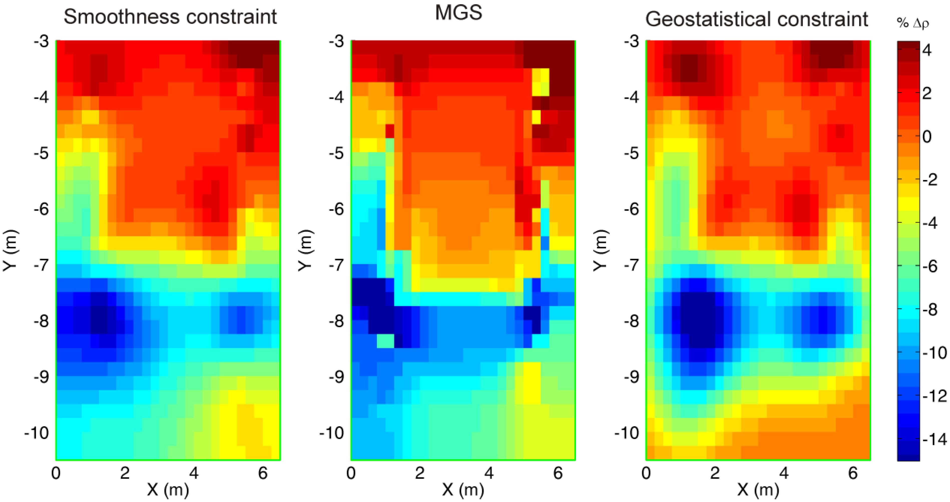
5.3. ERT Survey Design

A distinction has to be done between surface and cross-borehole ERT. Surface ERT is particularly suited for monitoring application. It is non-invasive since it only requires electrodes at the ground surface. However, surface measurements suffer from poor resolution at depth [45,113,114] even if Robert et al. [51] successfully managed to follow a salt tracer in fractures at a depth of 20 to 30 m. Hermans et al. [74] propose guidelines deduced from their study case to design surface arrays for monitoring studies. Using 62 electrodes with an electrode spacing a, they successfully imaged a heat plume 3.33a thick, 4a wide and at a depth of 4a. The minimum temperature variations detected is dependent on the propagation of noise which was evaluated to about 10%.
Cross-borehole ERT enables to maintain sufficient resolution at depth. Electrodes can be fixed at the outer edge of the borehole or mounted on cables with the borehole fluid ensuring electrical contact (require a screen all along the borehole). In the latter case, the fluid contained in the borehole influences the measurement (borehole fluid effect, see [115]). The sensitivity is maximum near the borehole and decrease in the middle of the section. A minimum aspect ratio (equipped length over distance between boreholes) has to be maintained to ensure enough resolution in this part of the model. Using 13 electrodes in each borehole with an electrode spacing a, Hermans et al. [55] imaged a heterogeneous heat plume 5a thick and 4a wide, with an aspect ratio (ratio of the distance between boreholes over length equipped with electrode) of 0.75.
As an imaging technology resulting from a deterministic regularized inversion process, ERT is subject to limitations due to resolution patterns [116]. For surface ERT, the resolution pattern is strongly depth-dependent and the ability of the method to image temperature variations will rapidly decrease with depth. For cross-hole ERT, difference may appear in zones close to boreholes compare to the centered part of the channel. Those aspects have to be taken into account in the interpretation of tomograms transformed with petrophysical models.

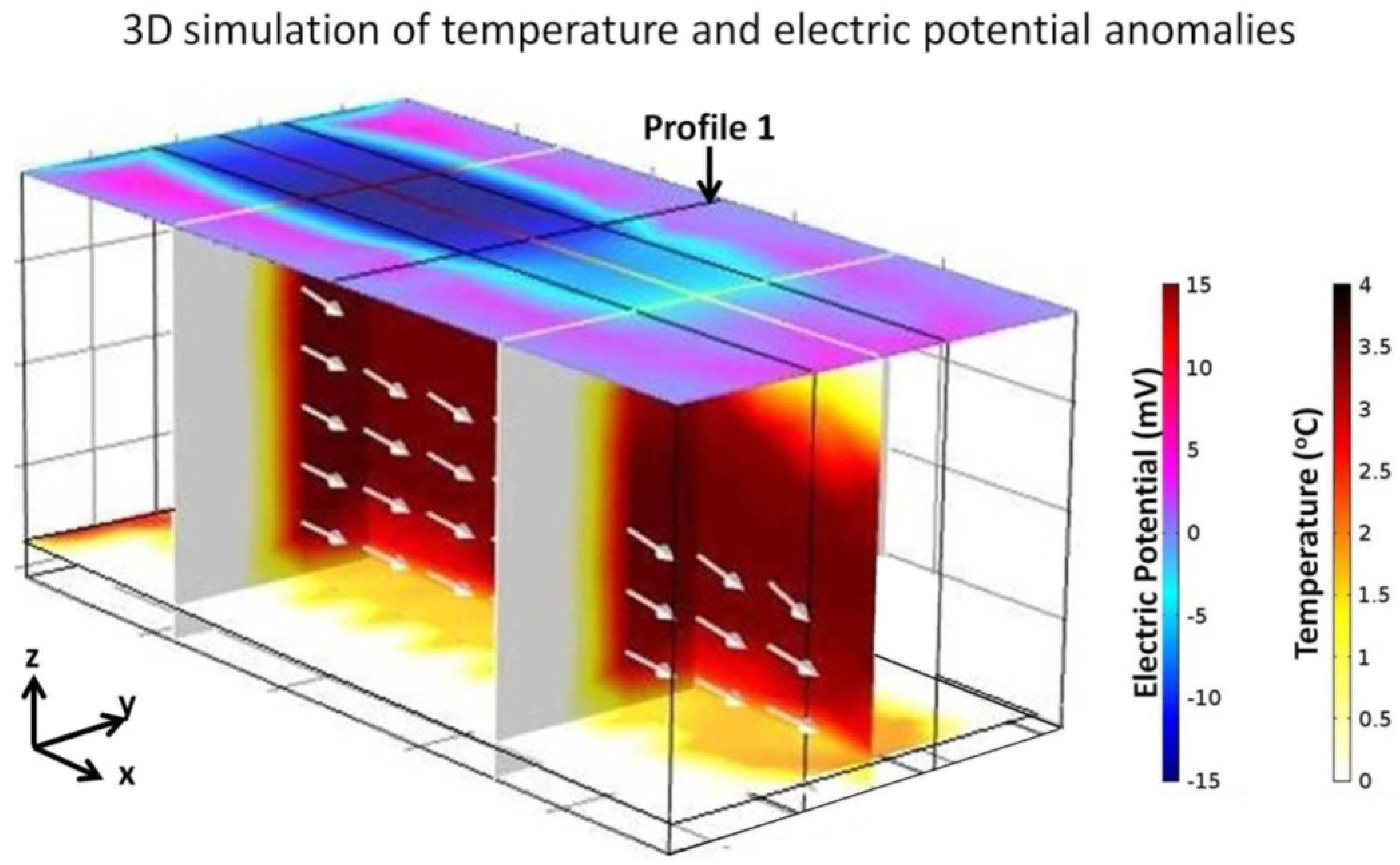
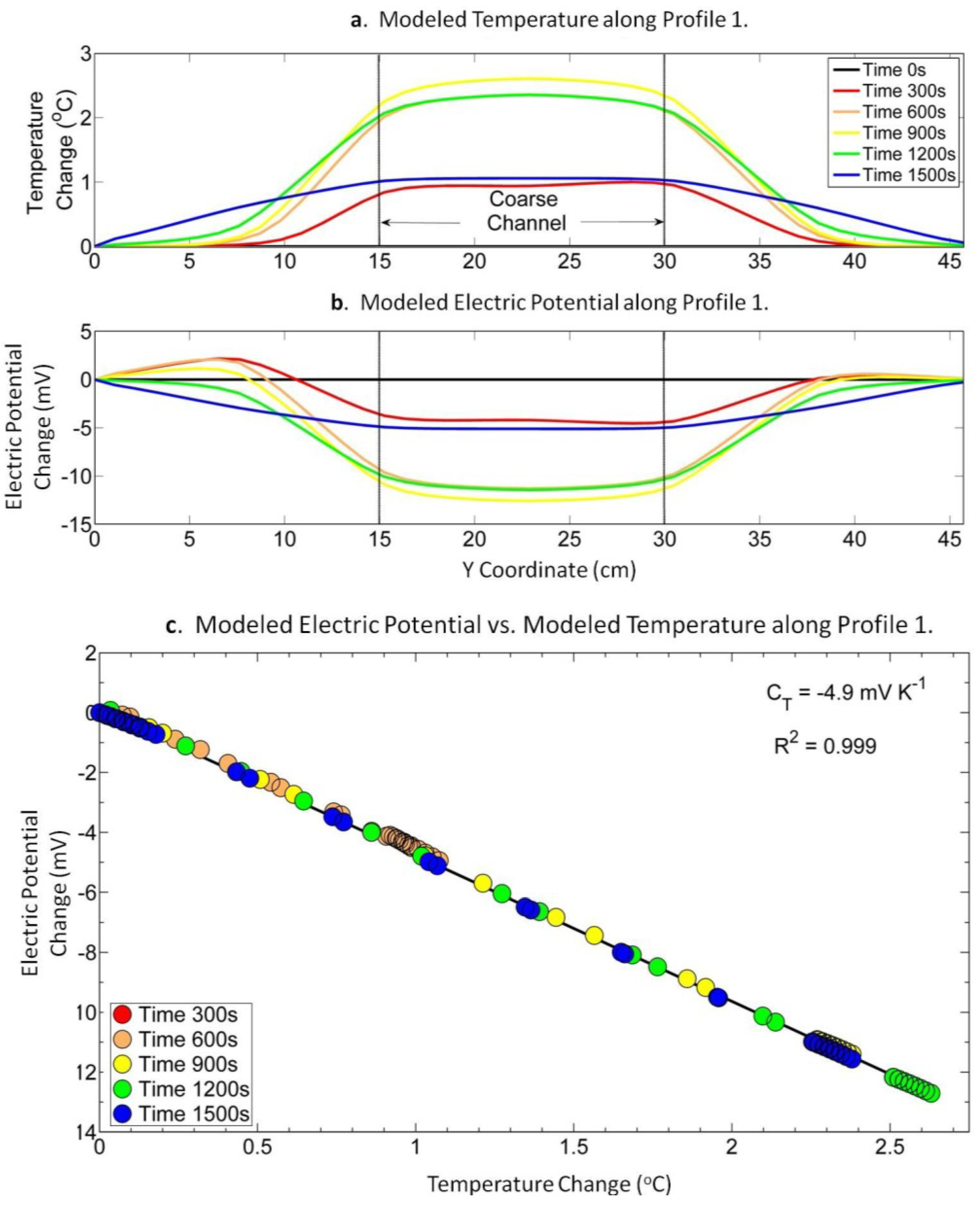
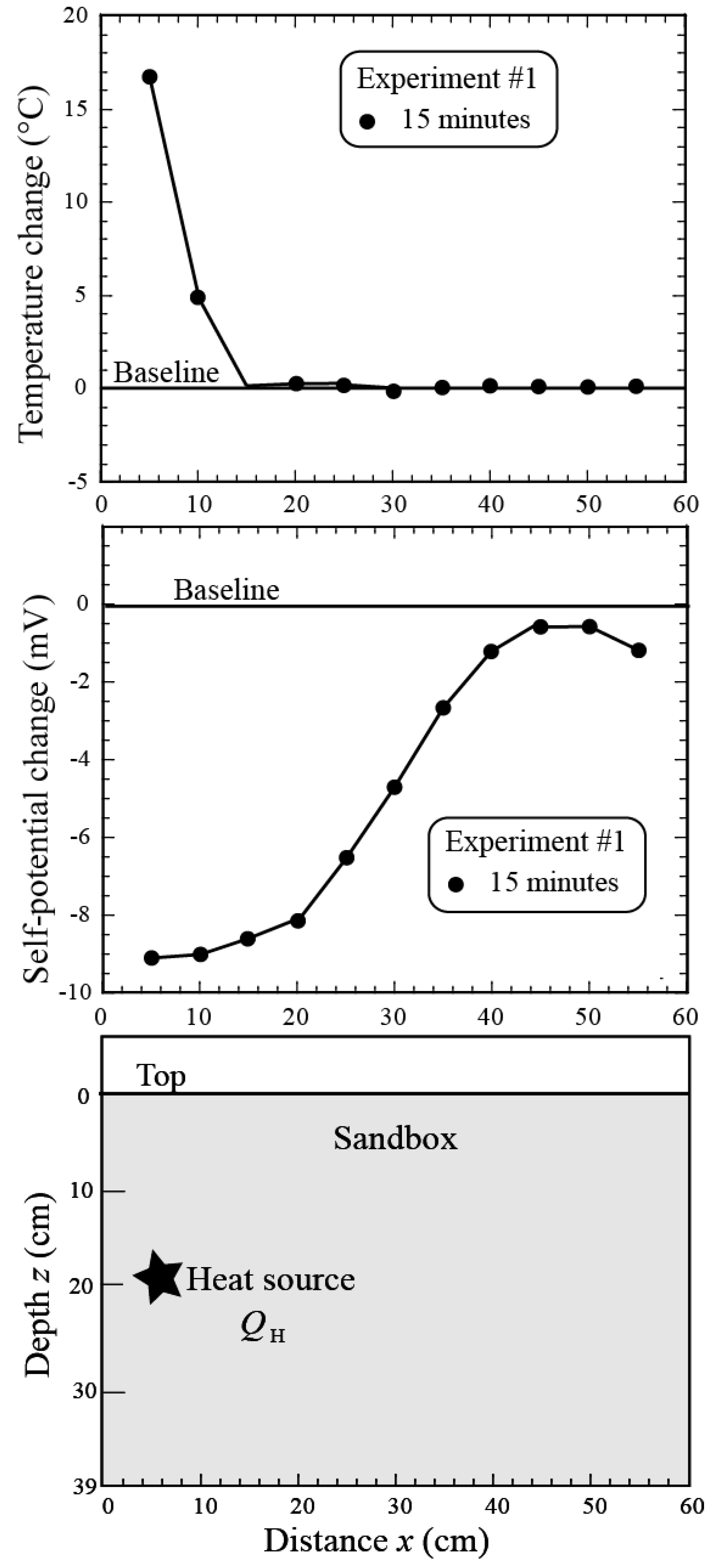
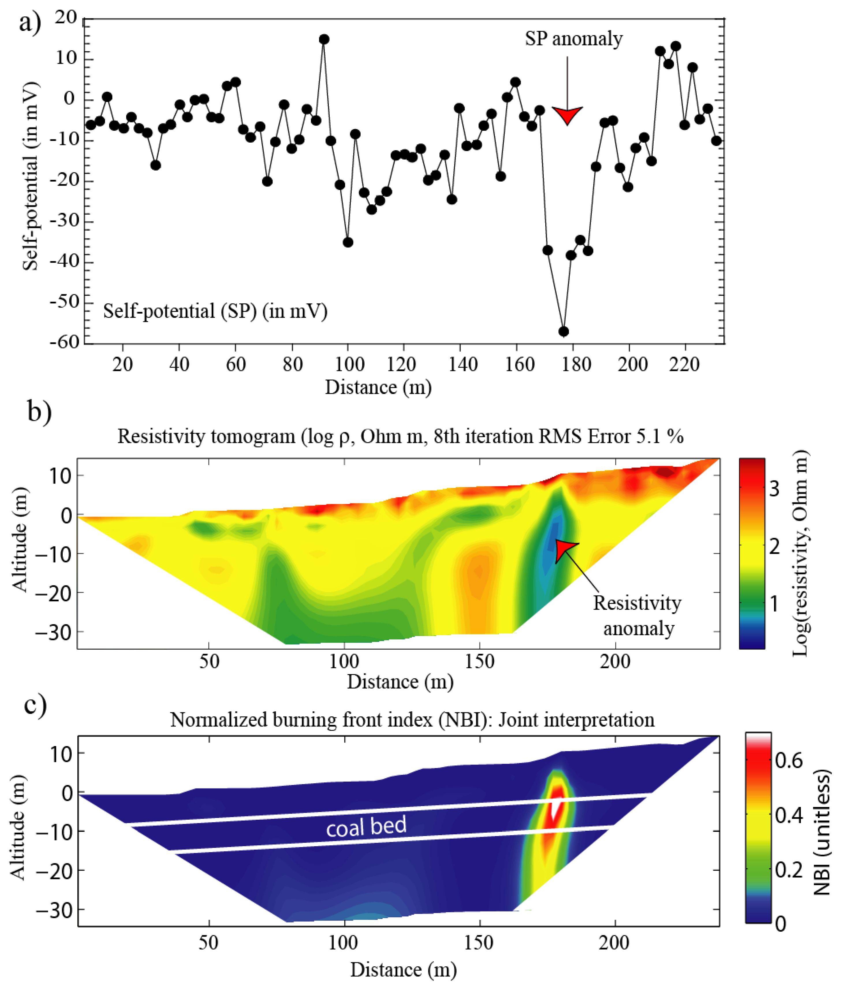
5.4. Sensitivity of Self-Potential Signals to Temperature

We first describe a sandbox experiment to estimate the amplitude of the self-potential anomalies associated with a heat source in absence of ground water flow. The sandbox was filled with a silica sand and demineralized water. We used two non-polarizing Pb/PbCl2 (Petiau) electrodes and an MX20 voltmeter (sensitivity 0.1 mV, internal impedance 100 MΩ) for the self-potential measurements. The reference electrode (ref) was located on the corner of the sandbox and its temperature was monitored over time (19.2 ± 0.1 °C). The other electrode was used to scan the electrical potential at the surface of the sand. The measurements were done in such a way that the temperature of the scanning electrode was kept constant in order to avoid artefacts in the experiment due to the difference of temperature between the scanning and the reference electrodes. Thermal probes and a digital thermometer were used to measure the temperature distribution. The thermal probes were inserted at a depth of 20 ± 1 cm prior the beginning of the experiment with a spacing of 5 cm (see Figure 11). The temperature was measured with an accuracy of 0.2 °C.
Self-potential and temperature data were gathered 5 min prior the introduction of the heat source to get reference profiles. The reference temperatures were 20.8 ± 0.1 °C. An amount of 9 g of a chemical heater was introduced in the tank at t = 0. The chemical heater was put dry at the bottom of a tube (2 cm in diameter) with dry sand above and a cap at the bottom. The tube was poured in the sandbox at a depth of 20 cm (see positions in Figure 11). These experiments will be referred as Experiments #1 and #2, respectively. The cap was pushed and the chemical heater poured in the sandbox and the tube removed. The chemical heater is a Flameless Ration Heater (FRH), which is a water-activated exothermic heater. The exothermic chemical reaction is:
Mg + 2H2O → Mg(OH)2 + H2 + Heat
with about 350 kilojoules of heat produced per kg. Then the temperature was monitored (at a depth of 20 cm) and the self-potential profiles were repeated for 80 min. We also monitored potential changes in the electrical conductivity of the pore water close to the chemical heater. Once corrected for temperature, we found no notable changes in the pore water conductivity.
A negative self-potential anomaly was observed above the heat source. Modeling indicates that the thermoelectric coupling coefficient was −0.5 mV per °C. This indicates that heat pulses can be measured non-intrusively and the result in self-potential signals can be inverted to retrieve some characteristic of the heat source or material properties such as the thermal diffusivity of the material.
We describe now a field example showing how self-potential and resistivity can be used in concert to locate a heat source in the ground. This heat source corresponds to a shallow coal seam fire located near Denver (CO, USA). The burning front is located in the Gorham subbituminous coal formation, located at a depth of about 10 m (Figure 12). Revil et al. [91] obtained new self-potential (with an anomaly of −50 mV) and resistivity data along the profile shown in Figure 12a,b. These data were analyzed jointly to localize along a single profile the position of the burning front (Figure 12c). This case study shows how self-potential and resistivity can be used to localize and eventually monitor a shallow heat source.
Figure 11. Distribution of temperature (at a depth of 20 cm), self-potential (at the top of the tank) at a given time after the introduction of the heat source QH at a depth of 20 cm in a sandbox. We have removed the temperature and self-potential distributions recorded prior the introduction of the heat source (modified after [91]).
Energies 07 05083 g011
Figure 12. Self-potential (SP) and resistivity data. (a) Self-potential data (79 stations performed at the ground surface) showing a self-potential anomaly at about 175 mV over the burning area; (b) Electrical resistivity tomogram (714 apparent resistivity data, Wenner-α, 79 electrodes, inverted with a Gauss-Newton algorithm with isotropic smoothing). Note the low resistivity anomaly (2 Ω·m) at about 175 m below the negative self-potential anomaly (−50 mV); (c) Burning front index based on the self-potential and resistivity values. High values correspond to a high probability zone in terms of recovering the position of the burning front. The depth of the maximum of the NBI coincides with the depth of the coal bed (approximately 10 m) (modified after [91]).
Energies 07 05083 g012

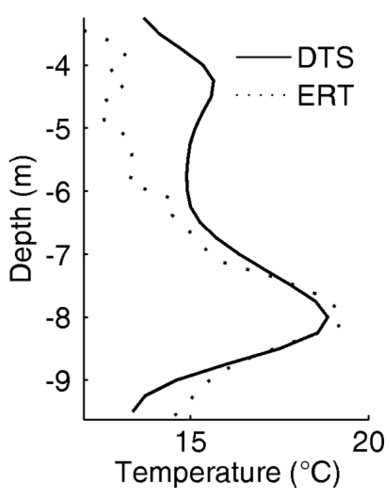
5.5. Using DTS to Measure Temperature

DTS systems were first used for fire or pipeline monitoring and used existing communication utilities rather than dedicated cables. However, in the last decade, the development of designed measuring systems in hydrogeology and geothermal systems has grown.
In the last decade, the method gained popularity among scientists concerned by hydrology. One of the main utilization of DTS in environmental hydrological studies concerns the surface water/groundwater interface. Groundwater temperature being almost constant with time, groundwater inflows may be detected with decrease in stream temperature in summer and increase in winter. Selker et al. [117] used the Raman-backscatter DTS along multimode fiber-optic cable with a temperature precision of 0.01 °C every meter to estimate stream temperature dynamics and groundwater inflows. Such a resolution is obtained by integrating signals over one hour time period. They used their results to derive groundwater temperatures and relative groundwater inflows. Lowry et al. [118] investigated groundwater discharge in a wetland stream using DTS. They repeated measurements every 15 min to propose a high resolution spatio-temporal monitoring of temperatures with the fiber buried in streambed sediments. They observe that temperature anomalies correlated with groundwater discharges with constant position in time. DTS temperatures correlated well with temperature data loggers.
DTS was also used to derive seepage rates in streams by determining the vertical temperature profiles. Vogt et al. [119] used DTS to get high resolution vertical temperature profiles in surface water sediments in order to derive seepage rates over depth and time. They wrapped the fiber around a PVC tube installed in the streambed sediments, as recommended by Selker et al. [94]. This configuration enables to refine the spatial resolution to about 5 mm instead of 1m which is the standard order of magnitude. Similarly, Mamer and Lowry [120] studied groundwater discharge to streams using paired fiber-optic cables. They propose a set up where two cables are parallel, one on the top of the other with a small vertical separation and tested this configuration in 10 m long sandbox. The overlapping time series measurements are then used to estimate fluxes along the stream longitudinally with the amplitude-shift method.
Applications in lakes, although more complex due to surface discharge area, exist too. Sebok et al. [121] used DTS to map spatial and temporal changes in temperature on a lakebed area to confirm the presence of a relatively high discharge of groundwater. The cable was spread out an area of 25 m × 6 m. The measurement through the seasons showed that the extent of the discharge zone was changing as well as its position relative to the shore. They also used a looped layout for multilevel lake temperature measurements.
The use of DTS in such applications has become standard. Consequently, many efforts are now done for the improvement of processing and interpretation of the spatio-temporal data sets. Lauer et al. [122] tested the fiber-optic DTS method to detect groundwater discharge to streams to assess uncertainty and limit of detections of the method. They implemented artificial upstream discharge in a stream with controlled inflow rates and temperatures. The sensitivity of the method appeared to be relatively high since DTS was able to detect discharge of 2% of natural flow. Krause and Blume [123] determined the impacts of seasonal variability in signal strengths and monitoring modes on the accuracy of fiber-optic DTS systems used to analyze thermal patterns in aquifer-river interfaces. They found that the stability in signal strength was better in winter and that two-way single ended averaging surveys were the best suited for monitoring. Mwakanyamale et al. [124] used fiber-optic DTS temperature measurements and propose a new approach combining spectral analysis and discriminant analysis to process DTS data and detect zones of exchange between surface water and groundwater more objectively. Blume et al. [125] compare upscaling approaches utilizing lacustrine groundwater discharge rates derived from fiber-optic DTS measurements. The major issue for lacustrine groundwater discharges lies in the identification of 2D patterns. Two transfer functions integrating DTS transects were developed and compared to a simple exponential decline of discharge rates perpendicular to the shoreline.
Ciocca et al. [126] used a fiber optic system to estimate soil moisture in alysimeter experiment. They used the metal around the fiber optic cable as an electrical resistance heater to generate heat pulse. The temperature of the soil was then monitored with DTS to derive the thermal conductivities of the soil. The latter were used to estimate water content through a calibrated petrophysical relationship that was compared to standard measurements of soil moisture with a relatively good agreement in wet conditions.
However, application of DTS in hydrogeology is not limited to surface or near-surface applications. Borehole applications, that are logistically similar to open loop systems, are also common. Hurtig et al. [127] reported one of the first utilization of DTS in hydrogeology. Cables were placed into a 40 m deep inclined borehole during injection of hot and cold water. With temperature profiling, a fracture was detected at the position of a sharp decrease in temperature. Macfarlane et al. [128] evaluated aquifer properties by heating fluid and stimulating flow (forced gradient) between wells. Temperatures were recorded using DTS in transient thermal conditions in injection and production wells, with short screen intervals. This thermal tracer test highlighted a zone of higher hydraulic conductivity between injection and pumping wells. Yamano and Goto [129] used DTS for long-term monitoring (6 years) of a deep borehole to investigate an active fault in Japan. They used a spatial resolution of 1 m with an expected resolution of 0.1 K. They coupled temperature measurement with cold water injection to detect leakage zones. Leaf et al. [130] monitored advective heat movement in borehole dilution tests with DTS. They tested several thermal tracer dilution experimental designs (continuous, pulse injection, single and multiple locations). Large screened intervals enabled them to use vertical temperature profiles as an indicator of vertical heterogeneity in the aquifer and of inflows from fractures and porous media. Read et al. [131] performed heat transport tests in fractured media using DTS for temperature monitoring in injection and pumping wells. They monitored thermal dilution tests to detect cross-flowing fractures and assess the cross flow rate. A cross well thermal tracer test was performed to identify the connection between boreholes through the fracture network. Banks et al. [132] used fiber-optic DTS to measure temperature profiles in open groundwater wells in fractured rock. They used electrical heating cables to heat the water in the well and create a temperature difference with the surrounding aquifer. Temperature profiles were used to identify active fracture zones within the aquifer. In open systems, the use of DTS to measure the temperature variations allows avoiding or at least minimizing forced convection effects in boreholes, which can occur when performing multilevel well sampling.
It is only very recently that such measures began to be made to characterize and eventually design geothermal systems, in particular for closed loop systems. Fujii et al. [133] first proposed to study thermal response test (TRT) with distributed temperature measured by optic fiber. However, they located the fiber outside of the U-pipe used for TRT. This configuration is not optimal because it is difficult to control the closeness of the fiber with the U-pipe in the ground material. Fujii et al. [134] included DTS measurements as a part of a thermal response test to determine ground thermal conductivities from 1 to 2 m thick layers. This time the cables are located inside the U-pipe. They show the reliability of the technique for the interpretation of thermal response test. Acuna et al. [135] similarly performed a distributed thermal response test with the fiber optic cables enclosed in the U-pipe. Such measures have helped to demonstrate and quantify a significant difference between the average thermal resistance of drilling obtained by thermal response tests and estimated thermal resistances along the drilling using distributed measurements.
With some adaptations, the use of DTS for deep geothermal systems is also possible. Reinsch et al. [136] installed a fiber-optic cable behind the cemented annulus of the casing of a high temperature geothermal well. Repeated measurements were used to detect mechanical, thermal and chemical degradation of the fiber. At high temperature, geothermal fluids may contain hydrogen which degrades the fiber and distort the optical signal through absorption. Mechanical stress may generate bending loss in the signal. Those conditions required to use specific cables with polyamide and hermetic carbon coatings. The measurements showed that the cable was damaged at several positions during installation but without preventing temperature measurements.
There is no limitation in the possible utilizations of the DTS technology. Selker et al. [94] reported several applications, including temperature measurements in a decommissioned mine shaft in Czech Republic and air-snow and air-water interfaces studies. Yilmaz and Karlik [95] incorporated DTS measurements for the monitoring of power cables.

6. Conclusions

Groundwater contributes to a major part in the production of geothermal energy, rather directly (GWHP or ATES systems) or indirectly (GSHP or BTES systems), by taking advantage of its inherent temperature stability for the operation of heat pumps. Very low temperature systems (<30 °C) are generally located at depth between 0 and 100 m, thus they are much more easily accessible and involve lower implementation costs than deeper high temperature systems (i.e., drilling costs). Moreover, very low temperature reservoirs, such as shallow aquifers, are relatively abundant in alluvial or coastal plains where urban development concentrates. At these depths, the subsurface is very heterogeneous and complex to characterize. The relatively wide range of natural variations both in terms of thermal and hydraulic properties makes designing efficient geothermal systems and predicting its impact on the environment challenging tasks.
In this context, new technologies are clearly needed to monitor the spatial and temporal distribution of temperature in the reservoir to: (1) better design the geothermal system and the monitoring network; (2) prevent any thermal feedback/recycling; and (3) image and control the thermal affected zone. Three emerging geophysical techniques in this field have been reviewed in this paper: electrical resistivity tomography (ERT) also known as electrical resistivity imaging (ERI) which allows to obtain 2D or 3D images of the temperature variations in the subsurface non-invasively; self-potential method (SP) which is a very fast method to map anomalies of the ambient electrical potential at the surface corresponding to temperature anomalies in the subsurface; and fiber-optic distributed temperature sensor (DTS) which provides linear measurements of temperature with centimetric resolution in boreholes. Whereas the latter provides a direct estimation of the temperature with little uncertainties, it requires the installation of boreholes to set up the fiber optics. The former two methods are mature enough to estimate temperature variations with respect to a given background in an almost non-invasive manner in the short term.
Challenges remain in terms of improving ERT imaging through advanced inversion algorithm and further strengthening the petrophysical relationships needed to obtain temperature changes for long term experiment. In this regard, research perspectives should focus on the incorporation of chemical and kinetic effects in the interpretation of the geophysical data.

Acknowledgments

We thank the F.R.S.-FNRS (Fonds de la Recherche Scientifique) and the Fondation Roi Baudouin—Prix Ernest Dubois (grant No. 2013-8126501-F002) for their financial support of Thomas Hermans. We also thank three anonymous reviewers for their comments and suggestions.

Author Contributions

Thomas Hermans contributed to the redaction of the sections related to ERT and time-lapse ERT, petrophysical considerations, DTS and previous works in ERT and DTS. He also ensured the coordination of the paper. Frédéric Nguyen contributed to the redaction of sections dedicated to ERT and time-lapse ERT as well as DTS and previous works in DTS. He also reviewed other sections of the paper. Tanguy Robert mainly contributed to the sections concerning ERT, time-lapse ERT and previous works in ERT. He also reviewed other parts of the paper. Finally, the major contributions of Andre Revil were the sections dedicated to SP, previous works in SP, and petrophysical considerations. He also reviewed other sections of the paper.

Conflicts of Interest

The authors declare no conflict of interest.

References

  1. Bayer, P.; Rybach, L.; Blum, P.; Brauchler, R. Review on life cycle environmental effects of geothermal power generation. Renew. Sustain. Energy Rev. 2013, 26, 446–463. [Google Scholar] [CrossRef]
  2. Saner, D.; Juraske, R.; Kübert, M.; Blum, P.; Hellweg, S.; Bayer, P. Is it only CO2 that matters? A life cycle perspective on shallow geothermal systems. Renew. Sustain. Energy Rev. 2010, 14, 1798–1813. [Google Scholar] [CrossRef]
  3. Andersson, O. ATES utilization in Sweden—An overview. In Proceedings of the MEGASTOCK’97 7th International Conference on Thermal Energy Storage, Sapporo, Japan, 18–20 June 1997; pp. 925–930.
  4. Vanhoudt, D.; Desmedt, J.; van Bael, J.; Robeyn, N.; Hoes, H. An aquifer thermal storage system in a Belgian hospital: Long-term experimental evaluation of energy and cost savings. Energy Build. 2011, 43, 3657–3665. [Google Scholar] [CrossRef]
  5. Blum, P.; Campillo, G.; Kölbel, T. Techno-economic and spatial analysis of vertical ground source heat pump systems in Germany. Energy 2011, 36, 3002–3011. [Google Scholar] [CrossRef]
  6. b>Haehnlein, S.; Bayer, P.; Ferguson, G.; Blum, P. Sustainability and policy for the thermal use of shallow geothermal energy. Energy Policy 2013, 59, 914–925. [Google Scholar] [CrossRef]
  7. Lund, J.W. Direct utilization of geothermal energy. Energies 2010, 3, 1443–1471. [Google Scholar] [CrossRef]
  8. European Commission. Horizon 2020: The EU Framework Programme for Research and Innovation. Secure, Clean and Efficient Energy. Available online: http://ec.europa.eu/programmes/horizon2020/en/h2020-section/secure-clean-and-efficient-energy (accessed on 11 August 2014).
  9. Lund, J.W.; Freeston, D.H.; Boyd, T.L. Direct application of geothermal energy: 2005 worldwide review. Geothermics 2005, 34, 691–727. [Google Scholar] [CrossRef]
  10. Allen, A.; Milenic, D. Low-enthalpy geothermal energy resources from groundwater in fluvioglacial gravels of buried valleys. Appl. Energy 2003, 74, 9–19. [Google Scholar] [CrossRef]
  11. b>Haehnlein, S.; Bayer, P.; Blum, P. International legal status of the use of shallow geothermal energy. Renew. Sustain. Energy Rev. 2010, 14, 2611–2625. [Google Scholar] [CrossRef]
  12. Mattsson, N.; Steinmann, G.; Laloui, L. Advanced compact device for the in situ determination of geothermal characteristics of soils. Energy Build. 2008, 40, 1344–1352. [Google Scholar] [CrossRef]
  13. Raymond, J.; Therrien, R.; Gosselin, L.; Lefebvre, R. A review of thermal response test analysis using pumping test concepts. Groundwater 2011, 49, 932–945. [Google Scholar] [CrossRef]
  14. Haffen, S.; Geraud, Y.; Diraison, M.; Dezayes, C. Determination of fluid-flow zones in a geothermal sandstone reservoir using thermal conductivity and temperature logs. Geothermics 2013, 46, 32–41. [Google Scholar] [CrossRef] [Green Version]
  15. Busby, J.; Lewis, M.; Reeves, H.; Lawley, R. Initial geological considerations before installing ground source heat pump systems. Q. J. Eng. Geol. Hydrogeol. 2009, 42, 295–306. [Google Scholar]
  16. De Paly, M.; Hecht-Méndez, J.; Beck, M.; Blum, P.; Zell, A.; Bayer, P. Optimization of energy extraction for closed shallow geothermal systems using linear programming. Geothermics 2012, 43, 57–65. [Google Scholar]
  17. Liang, J.; Yang, Q.; Liu, L.; Li, X. Modeling and performance evaluation of shallow ground water heat pumps in Beijing plain, China. Energy Build. 2011, 43, 3131–3138. [Google Scholar] [CrossRef]
  18. Lo Russo, S.; Civita, M.V. Open-loop groundwater heat pumps development for large buildings: A case study. Geothermics 2009, 38, 335–345. [Google Scholar]
  19. Molson, J.W.; Frind, E.O.; Palmer, C.D. Thermal energy storage in an unconfined aquifer: 2. Model development, validation and application. Water Resour. Res. 1992, 28, 2857–2867. [Google Scholar]
  20. Palmer, C.D.; Blowes, D.W.; Frind, E.O.; Molson, J.W. Thermal energy storage in an unconfined aquifer: 1. Field injection experiment. Water Resour. Res. 1992, 28, 2845–2866. [Google Scholar] [CrossRef]
  21. Warner, D.L.; Algan, U. Thermal impact of residential ground-water heat pumps. Groundwater 1984, 22, 6–12. [Google Scholar] [CrossRef]
  22. Bonte, M. Impacts of Shallow Geothermal Energy Storage on Groundwater Quality—A Hydrochemical and Hydromicrobial Study of the Effects of Ground Source Heat Pumps and Aquifer Thermal Storage. Ph.D. Thesis, VU University Amsterdam, Amsterdam, The Netherlands, 2013. [Google Scholar]
  23. Garnier, F. Contribution à l’évaluation Biogéochimique des Impacts liés à l’exploitation Géothermique des Aquifères Superficiels: Expérimentations et Simulations à l’échelle d’un Pilote et d’installations Réelles. Ph.D. Thesis, Bureau de Recherche Géologique et Minière¡ªInstitut des Sciences de la Terre d’Orléans, Université d’Orléans, Orléans, France, 2012. [Google Scholar]
  24. Jesuβek, A.; Grandel, S.; Dahmke, A. Impacts of subsurface heat storage on aquifer hydrogeochemistry. Environ. Earth Sci. 2013, 69, 1999–2012. [Google Scholar]
  25. Brielmann, H.; Griebler, C.; Schmidt, S.I.; Michel, R.; Lueders, T. Effects of thermal energy discharge on shallow groundwater ecosystems. FEMS Microbiol. Ecol. 2009, 68, 273–286. [Google Scholar] [CrossRef] [PubMed]
  26. Lerm, S.; Westphal, A.; Miethling-Graff, R.; Alawi, M.; Seibt, A.; Wolfgramm, M.; Würdemann, H. Thermal effects on microbial composition and microbiologically induced corrosion and mineral precipitation affecting operation of a geothermal plant in a deep saline aquifer. Extremophiles 2013, 17, 311–327. [Google Scholar] [CrossRef] [PubMed]
  27. Vetter, A.; Mangelsdorf, K.; Wolfgramm, M.; Rauppach, K.; Schettler, G.; Vieth-Hillebrand, A. Variations in fluid chemistry and membrane phospholipid fatty acid composition of the bacterial community in a cold storage groundwater system during clogging events. Appl. Geochem. 2012, 27, 1278–1290. [Google Scholar] [CrossRef]
  28. Lo Russo, S.; Gnavia, L.; Roccia, E.; Taddia, G.; Verda, V. Groundwater Heat Pump (GWHP) system modeling and Thermal Affected Zone (TAZ) prediction reliability: Influence of temporal variations in flow discharge and injection temperature. Geothermics 2014, 51, 103–112. [Google Scholar]
  29. Lo Russo, S.; Taddia, G.; Verda, V. Development of the thermally affected zone (TAZ) around a groundwater heat pump (GWHP) system: A sensitivity analysis. Geothermics 2012, 43, 66–74. [Google Scholar]
  30. Gao, Q.; Zhou, X.-Z.; Jiang, Y.; Chen, X.-L.; Yan, Y.-Y. Numerical simulation of the thermal interaction between pumping and injecting well groups. Appl. Therm. Eng. 2013, 51, 10–19. [Google Scholar] [CrossRef]
  31. Milnes, E.; Perrochet, P. Assessing the impact of thermal feedback and recycling in open-loop groundwater heat pump (GWHP) systems: A complementary design tool. Hydrogeol. J. 2013, 21, 505–514. [Google Scholar]
  32. Anderson, M.P. Heat as a ground water tracer. Groundwater 2005, 43, 951–968. [Google Scholar] [CrossRef]
  33. Wikdemeersch, S.; Jamin, P.; Orban, P.; Hermans, T.; Nguyen, F.; Brouyère, S.; Dassargues, A. Coupling heat and chemical tracer experiments for estimating heat transfer parameters in shallow alluvial aquifers. J. Contam. Hydrol. 2014. submitted. [Google Scholar]
  34. Saar, M.O. Review: Geothermal heat as a tracer of large-scale groundwater flow and as a means to determine permeability fields. Hydrogeol. J. 2011, 19, 31–52. [Google Scholar] [CrossRef]
  35. Giambastiani, B.M.S.; Colombanii, N.; Mastrocicco, M. Limitation of using heat as a groundwater tracer to define aquifer properties: Experiment in a large tank model. Environ. Earth Sci. 2013, 70, 719–728. [Google Scholar] [CrossRef]
  36. Vandenbohede, A.; Hermans, T.; Nguyen, F.; Lebbe, L. Shallow heat injection and storage experiment: Heat transport simulation and sensitivity analysis. J. Hydrol. 2011, 409, 262–272. [Google Scholar] [CrossRef]
  37. Vandenbohede, A.; Louwyck, A.; Lebbe, L. Conservative solute versus heat transport in porous media during push-pull tests. Transp. Porous Med. 2009, 76, 265–287. [Google Scholar] [CrossRef]
  38. Brouyère, S. Etude et Modélisation du Transport et du Piégeage des Solutés en Milieu Souterrain Variablement Saturé. Ph.D. Thesis, University of Liege, Liege, Belgium, 2001. [Google Scholar]
  39. b>Jardani, A.; Revil, A.; Dupont, J.P. Stochastic joint inversion of hydrogeophysical data for salt tracer test monitoring and hydraulic conductivity imaging. Adv. Water Resour. 2013, 52, 62–77. [Google Scholar] [CrossRef]
  40. b>Hayley, K.; Bentley, L.R.; Gharibi, M.; Nightingale, M. Low temperature dependence of electrical resistivity: Implications for near surface geophysical monitoring. Geophys. Res. Lett. 2007, 34. [Google Scholar] [CrossRef]
  41. Revil, A.; Cathles, L.M.; Losh, S.; Nunn, J.A. Electrical conductivity in shaly sands with geophysical applications. J. Geophys. Res. 1998, 103, 23925–23936. [Google Scholar] [CrossRef]
  42. Waxman, M.H.; Smits, L.J.M. Electrical conductivities in oil-bearing shaly sands. Soc. Pet. Eng. J. 1968, 8, 107–122. [Google Scholar] [CrossRef]
  43. Vereecken, H.; Binley, A.; Cassiani, G.; Revil, A.; Titov, K. Applied Hydrogeophysics. NATO Science Series: IV Earth and Environmental Sciences; Springer: Berlin, Germany, 2006. [Google Scholar]
  44. Hermans, T.; Vandenbohede, A.; Lebbe, L.; Martin, R.; Kemna, A.; Beaujean, J.; Nguyen, F. Imaging artificial salt water infiltration using electrical resistivity tomography constrained by geostatistical data. J. Hydrol. 2012, 438–439, 168–180. [Google Scholar]
  45. Nguyen, F.; Kemna, A.; Antonsson, A.; Engesgaard, P.; Kuras, O.; Ogilvy, R.; Gisbert, J.; Jorreto, S.; Pulido-Bosch, A. Characterization of seawater intrusion using 2D electrical imaging. Near Surf. Geophys. 2009, 7, 377–390. [Google Scholar] [CrossRef] [Green Version]
  46. Binley, A.; Winship, P.; West, L.J.; Pokar, M.; Middleton, R. Seasonal variation of moisture content in unsaturated sandstone inferred from borehole radar and resistivity profiles. J. Hydrol. 2002, 267, 160–172. [Google Scholar] [CrossRef]
  47. Chambers, J.E.; Gunn, D.A.; Wilkinson, P.B.; Meldrum, P.I.; Haslam, E.; Holyoake, S.; Kirkham, M.; Kuras, O.; Merrit, A.; Wragg, J. 4D electrical resistivity tomography monitoring of soil moisture dynamics in an operational railway embankment. Near Surf. Geophys. 2014, 12, 61–72. [Google Scholar] [Green Version]
  48. Atekwana, E.A.; Sauck, W.A.; Werkema, D.D., Jr. Investigations of geoelectrical signatures at a hydrocarbon contaminated site. J. Appl. Geophys. 2000, 44, 167–180. [Google Scholar] [CrossRef]
  49. Chambers, J.E.; Wilkinson, P.B.; Wealthall, G.P.; Loke, M.H.; Dearden, R.; Wilson, R.; Allen, D.; Ogilvy, R.D. Hydrogeophysical imaging of deposit heterogeneity and groundwater chemistry changes during DNAPL source zone bioremediation. J. Contam. Hydrol. 2010, 118, 43–61. [Google Scholar] [CrossRef] [PubMed] [Green Version]
  50. Kemna, A.; Kulessa, B.; Vereecken, H. Imaging and characterization of subsurface solute transport using electrical resistivity tomography (ERT) and equivalent transport models. J. Hydrol. 2002, 267, 125–146. [Google Scholar] [CrossRef]
  51. Robert, T.; Caterina, D.; Deceuster, J.; Kaufmann, O.; Nguyen, F. A salt tracer test monitored with surface ERT to detect preferential flow and transport paths in fractured/karstified limestones. Geophysics 2012, 77, B55–B67. [Google Scholar] [CrossRef]
  52. Schön, J.H. Physical Properties of Rocks, Fundamentals and Principles of Petrophysics. In Handbook of Geophysical Exploration, Seismic Exploration; Helbig, K., Treitel, S., Eds.; Elsevier: Amsterdam, The Netherlands, 2004. [Google Scholar]
  53. Revil, A.; Karaoulis, M.; Johnson, T.; Kemna, A. Review: Some low-frequency electrical methods for subsurface characterization and monitoring in hydrogeology. Hydrogeol. J. 2012, 20, 617–658. [Google Scholar] [CrossRef]
  54. Binley, A.; Kemna, A. DC resistivity and induced polarization methods. In Hydrogeophysics; Springer: Berlin, Germany, 2005; pp. 129–156. [Google Scholar]
  55. Hermans, T.; Wildemeersch, S.; Jamin, P.; Orban, P.; Brouyère, S.; Dassargues, A.; Nguyen, F. Quantitative temperature monitoring of a heat tracing experiment using cross-borehole ERT. Geothermics 2015, 53, 14–26. [Google Scholar] [CrossRef]
  56. Tikhonov, A.N.; Arsenin, V.A. Solution of Ill-Posed Problems; Winston & Sons: Washington, DC, USA, 1977. [Google Scholar]
  57. Sen, P.N.; Goode, P.A. Influence of temperature on electrical conductivity on shaly sands. Geophysics 1992, 46, 781–795. [Google Scholar] [CrossRef]
  58. Hayley, K.; Bentley, L.R.; Pidlisecky, A. Compensating for temperature variations in time-lapse electrical resistivity difference imaging. Geophysics 2010, 75, WA51–WA59. [Google Scholar] [CrossRef]
  59. Ma, R.; McBratney, A.; Whelan, B.; Minasny, B.; Short, M. Comparing temperature correction models for soil electrical conductivity measurement. Precis. Agric. 2011, 12, 55–66. [Google Scholar] [CrossRef]
  60. Sherrod, L.; Sauck, W.; Werkema, D.D., Jr. A low-cost, in-situ resistivity and temperature monitoring system. Ground Water Monit. Remediat. 2012, 32, 31–39. [Google Scholar] [CrossRef]
  61. Loke, M.H.; Dahlin, T.; Rucker, D.F. Smoothness-constrained time-lapse inversion of data from 3D resistivity survey. Near Surf. Geophys. 2014, 12, 5–24. [Google Scholar]
  62. Miller, C.; Routh, P.; Brosten, T.; McNamara, J. Application of time-lapse ERT imaging to watershed characterization. Geophysics 2008, 73, G7–G17. [Google Scholar] [CrossRef]
  63. Daily, W.; Ramirez, A.; LaBrecque, D.; Nitao, J. Electrical resistivity tomography of vadose water movement. Water Resour. Res. 1992, 28, 1429–1442. [Google Scholar] [CrossRef]
  64. LaBrecque, D.J.; Yang, X. Difference inversion of ERT data: A fast inversion method for 3-D in-situ monitoring. J. Environ. Eng. Geophys. 2001, 6, 83–90. [Google Scholar]
  65. Nguyen, F.; Hermans, T.; Robert, T. Minimum gradient support and geostatistics regularization approaches for inverting time-lapse data. In Proceedings of 2nd International Workshop on Geoelectrical Monitoring, Vienna, Austria, 4–6 December 2013.
  66. Karaoulis, M.; Tsourlos, P.; Kim, J.-H.; Revil, A. 4D time-lapse ERT inversion: Introducing combined time and space constraints. Near Surf. Geophys. 2014, 12, 25–34. [Google Scholar] [CrossRef]
  67. Karaoulis, M.C.; Kim, J.H.; Tsourlos, P.I. 4D active time constrained resistivity inversion. J. Appl. Geophys. 2011, 73, 25–34. [Google Scholar] [CrossRef]
  68. Revil, A.; Skold, M.; Karaoulis, M.; Schmutz, M.; Hubbard, S.S.; Mehlhorn, T.L.; Watson, D.B. Hydrogeophysical investigations of the former S-3 ponds contaminant plumes, Oak Ridge Integrated Field Research Challenge site, Tennessee. Geophysics 2013, 78, EN29–EN41. [Google Scholar] [CrossRef]
  69. Pidlisecky, A.; Haber, E.; Knight, R. RESINVM3D: A 3D resistivity inversion package. Geophysics 2007, 72, H1–H10. [Google Scholar] [CrossRef]
  70. Kemna, A. Tomographic Inversion of Complex Resistivity: Theory and Application. Ph.D. Thesis, University of Bochum, Bochum, Germany, 2000. [Google Scholar]
  71. Nimmer, R.E.; Osiensky, J.L.; Binley, A.M.; Williams, B.C. Three-dimensional effects causing artifacts in two-dimensional, cross-borehole, electrical imaging. J. Hydrol. 2008, 359, 59–70. [Google Scholar] [CrossRef]
  72. Vandenborght, J.; Kemna, A.; Hardelauf, H.; Vereecken, H. Potential of electrical resistivity tomography to infer aquifer transport characteristics from tracer studies: A synthetic case study. Water Resour. Res. 2005, 41. [Google Scholar] [CrossRef]
  73. LaBrecque, D.J.; Miletto, M.; Daily, W.; Ramirez, A.; Owen, E. The effects of noise on Occam’s inversion of resistivity tomography data. Geophysics 1996, 61, 538–548. [Google Scholar] [CrossRef]
  74. Hermans, T.; Vandenbohede, A.; Lebbe, L.; Nguyen, F. A shallow geothermal experiment in a sandy aquifer monitored using electric resistivity tomography. Geophysics 2012, 77, B11–B21. [Google Scholar] [CrossRef]
  75. Irving, J.; Singha, K. Stochastic inversion of tracer test and electrical geophysical data to estimate hydraulic conductivities. Water Resour. Res. 2010, 46. [Google Scholar] [CrossRef]
  76. Kowalsky, M.B.; Finsterle, S.; Peterson, J.; Hubbard, S.; Rubin, Y.; Majer, E.; Ward, A.; Gee, G. Estimation of field-scale soil hydraulic and dielectric parameters through joint inversion of GPR and hydrological data. Water Resour. Res. 2005, 41. [Google Scholar] [CrossRef]
  77. Loke, M.H.; Acworth, I.; Dahlin, T. A comparison of smooth and blocky inversion methods in 2D electrical imaging surveys. Explor. Geophys. 2003, 34, 182–187. [Google Scholar] [CrossRef]
  78. Blaschek, R.; Hördt, A.; Kemna, A. A new sensitivity-controlled focusing regularization scheme for the inversion of induced polarization based on the minimum gradient support. Geophysics 2008, 73, F45–F54. [Google Scholar] [CrossRef]
  79. Doetsch, J.; Linde, N.; Pessognelli, M.; Green, A.G.; Günther, T. Constraining 3-D electrical resistance tomography with GPR reflection data for improved aquifer characterization. J. Appl. Geophys. 2012, 78, 68–76. [Google Scholar] [CrossRef]
  80. Zhou, J.; Revil, A.; Karaoulis, M.; Hale, D.; Doetsch, J.; Cuttler, S. Image-guided inversion of electrical resistivity data. Geophys. J. Int. 2014, 197, 292–309. [Google Scholar] [CrossRef]
  81. Caterina, D.; Hermans, T.; Nguyen, F. Case studies of prior information in electrical resistivity tomography: Comparison of different approaches. Near Surf. Geophys. 2014, 12, 451–465. [Google Scholar] [CrossRef]
  82. Kyriakidis, P.C.; Journel, A.G. Geostatistical space-time models: A review. Math. Geol. 1999, 31, 651–684. [Google Scholar] [CrossRef]
  83. Revil, A. Effective conductivity and permittivity of unsaturated porous materials in the frequency range 1 mHz–1 GHz. Water Resour. Res. 2013, 49, 306–327. [Google Scholar] [CrossRef] [PubMed]
  84. Revil, A.; Schwaeger, H.; Cathles, L.M.; Manhardt, P.D. Streaming potential in porous media: 2. Theory and application to geothermal systems. J. Geophys. Res. 1999, 104, 20033–20048. [Google Scholar] [CrossRef]
  85. Archie, G.E. The electrical resistivity log as an aid in determining some reservoir characteristics. Trans. AIME 1942, 146, 54–62. [Google Scholar] [CrossRef]
  86. Revil, A. On charge accumulations in heterogeneous porous materials under the influence of an electrical field. Geophysics 2013, 78, D271–D291. [Google Scholar] [CrossRef]
  87. Sorensen, J.A.; Glass, G.E. Ion and temperature dependence of electrical conductance for natural waters. Anal. Chem. 1987, 59, 1594–1597. [Google Scholar] [CrossRef]
  88. Jardani, A.; Revil, A.; Bolève, A.; Dupont, J.P.; Barrash, W.; Malama, B. Tomography of groundwater flow from self-potential (SP) data. Geophys. Res. Lett. 2006, 33. [Google Scholar] [CrossRef]
  89. Revil, A.; Mahardika, H. Coupled hydromechanical and electromagnetic disturbances in unsaturated clayey materials. Water Resour. Res. 2013, 49, 744–766. [Google Scholar] [CrossRef] [PubMed]
  90. Leinov, E.; Vinogradov, J.; Jackson, M.D. Salinity dependence of the thermoelectric coupling coefficient in brine-saturated sandstones. Geophys. Res. Lett. 2010, 37. [Google Scholar] [CrossRef]
  91. Revil, A.; Karaoulis, M.; Srivastava, S.; Byrdina, S. Thermoelectric self-potential and resistivity data localize the burning front of underground coal fires. Geophysics 2013, 78, B259–B273. [Google Scholar] [CrossRef]
  92. Sill, W.R. Self-potential modeling from primary flows. Geophysics 1983, 48, 76–86. [Google Scholar] [CrossRef]
  93. Ikard, S.J.; Revil, A. Self-potential monitoring of a thermal pulse advecting through a preferential flow path. J. Hydrol. 2014, 2014. [Google Scholar] [CrossRef]
  94. Selker, J.S.; Thévenaz, L.; Huwald, H.; Mallet, A.; Luxemburg, W.; van de Giesen, N.; Stejskal, M.; Zeman, J.; Westhoff, M.; Parlange, M.B. Distributed fiber-optic temperature sensing for hydrologic systems. Water Resour. Res. 2006, 42. [Google Scholar] [CrossRef] [Green Version]
  95. Yilmaz, G.; Karlik, S.E. A distributed optical fiber sensor for temperature detection in power cables. Sens. Actuators A 2006, 125, 148–155. [Google Scholar] [CrossRef]
  96. Tyler, S.W.; Selker, J.S.; Hausner, M.B.; Hatch, C.E.; Torgersen, T.; Thodal, C.E.; Schladow, S.G. Environmental temperature sensing using Raman spectra DTS fiber-optic methods. Water Resour. Res. 2009, 45. [Google Scholar] [CrossRef] [Green Version]
  97. Arango-Galván, C.; Prol-Ledesma, R.M.; Flores-Márquez, E.L.; Canet, C.; Villanueva Estrada, R.E. Shallow submarine and subaerial, low-enthalpy hydrothermal manifestations on Punta Banda, Baja California, Mexico: Geophysical and geochemical characterization. Geothermics 2011, 40, 102–111. [Google Scholar]
  98. Bruno, P.P.G.; Paoletti, V.; Grimaldi, M.; Rapolla, A. Geophysical exploration for geothermal low enthalpy resources in Lipari Island, Italy. J. Volcanol. Geotherm. Res. 2000, 98, 173–188. [Google Scholar] [CrossRef]
  99. Garg, S.K.; Pritchett, J.W.; Wannamaker, P.E.; Combs, J. Characterization of geothermal reservoirs with electrical surveys: Beowave geothermal field. Geothermics 2007, 36, 487–517. [Google Scholar] [CrossRef]
  100. Pérez Flores, M.A.; Gomez Trevino, E. Dipole-dipole resistivity imaging of the Ahuachapan-Chipilapa geothermal field, El Salvador. Geothermics 1997, 26, 657–680. [Google Scholar]
  101. Revil, A.; Finizola, A.; Ricci, T.; Delcher, E.; Peltier, A.; Barde-Cabusson, S.; Avard, G.; Bailly, T.; Bennati, L.; Byrdina, S.; et al. Hydrogeology of Stromboli volcano, Aeolian Islands (Italy) from the interpretation of resistivity tomograms, self-potential, soil temperature and soil CO2 concentration measurements. Geophys. J. Int. 2011, 186, 1078–1094. [Google Scholar] [CrossRef]
  102. Revil, A.; Johnson, T.C.; Finizola, A. Three-dimensional resistivity tomography of Vulcan’s forge, Vulcano Island, southern Italy. Geophys. Res. Lett. 2010, 37. [Google Scholar] [CrossRef]
  103. Benderitter, Y.; Tabbagh, J. Heat storage in a shallow confined aquifer: Geophysical tests to detect the resulting anomaly and its evolution with time. J. Hydrol. 1982, 56, 85–98. [Google Scholar] [CrossRef]
  104. Ramirez, A.; Daily, W.; LaBrecque, D.; Owen, E.; Chesnut, D. Monitoring an underground steam injection process using electrical resistance tomography. Water Resour. Res. 1993, 29, 73–87. [Google Scholar] [CrossRef]
  105. Ramirez, A.; Chesnut, D.A.; Daily, W.D. Using Electrical Resistance Tomography to Map Subsurface Temperatures. U.S. Patent US5346307 A, 3 June 1993. [Google Scholar]
  106. LaBrecque, D.J.; Ramirez, A.L.; Daily, W.D.; Binley, A.M.; Schima, S.A. ERT monitoring of environmental remediation processes. Meas. Sci. Technol. 1996, 7, 375–383. [Google Scholar] [CrossRef]
  107. Müller, K.; Vanderborght, J.; Englert, A.; Kemna, A.; Huisman, J.A.; Rings, J.; Vereecken, H. Imaging and characterization of solute transport during two tracer tests in a shallow aquifer using electrical resistivity tomography and multilevel groundwater samplers. Water Resour. Res. 2010, 46. [Google Scholar] [CrossRef]
  108. Firmbach, L.; Giordano, N.; Comina, C.; Mandrone, G.; Kolditz, O.; Vienken, T.; Dietrich, P. Experimental heat flow propagation within porous media using electrical resistivity tomography x(ERT). In Proceedings of the European Geothermal Congress 2013, Pisa, Italy, 3–7 June 2013.
  109. Supper, R.; Ottowitz, D.; Jochum, B.; Römer, A.; Pfeiler, S.; Kauer, S.; Keushnig, M.; Ita, A. Geoelctrical monitoring of frozen ground and permafrost in alpine areas: Field studies and considerations towards an improved measuring technology. Near Surf. Geophys. 2014, 12, 93–115. [Google Scholar]
  110. Auken, E.; Doetsch, J.; Fiandaca, G.; Christiansen, A.V.; Gazoty, A.; Cahill, A.G.; Jakobsen, R. Imaging subsurface migration of dissolved CO2 in a shallow aquifer using 3-D time-lapse electrical resistivity tomography. J. Appl. Geophys. 2013, 101, 31–41. [Google Scholar] [CrossRef]
  111. Hermans, T.; Daoudi, M.; Vandenbohede, A.; Robert, T.; Caterina, D.; Nguyen, F. Comparison of temperature estimates from heat transport model and electrical resistivity tomography during a shallow heat injection and storage experiment. Ber. Geol. Bundesanst. 2012, 93, 43–48. [Google Scholar]
  112. Robert, T.; Hermans, T.; Dumont, G.; Nguyen, F.; Rwabuhungu, D.E. Reliability of ERT-derived temperature: Insights from laboratory measurements. Near Surf. Geosci. 2013, 2013. [Google Scholar] [CrossRef]
  113. Caterina, D.; Beaujean, J.; Robert, T.; Nguyen, F. A comparison study of different image appraisal tools for electrical resistivity tomography. Near Surf. Geophys. 2013, 11, 639–657. [Google Scholar] [CrossRef]
  114. Perri, M.T.; Cassiani, G.; Gervasio, I.; Deiana, R.; Binley, A. A saline tracer test monitored via both surface and cross-borehole electrical resistivity tomography: Comparison of time-lapse results. J. Appl. Geophys. 2012, 79, 6–16. [Google Scholar] [CrossRef]
  115. Doetsch, J.A.; Coscia, I.; Greenhalgh, S.; Linde, N.; Green, A.; Günther, T. The borehole-fluid effect in electrical resistivity imaging. Geophysics 2010, 75, F107–F114. [Google Scholar] [CrossRef]
  116. Day-Lewis, F.D.; Singha, K.; Binley, A.M. Applying petrophysical models to radar travel time and electrical resistivity tomograms: Resolution-dependent limitations. J. Geophys. Res. Solid Earth 2005, 110. [Google Scholar] [CrossRef]
  117. Selker, J.; van de Giesen, N.; Westhoff, M.; Luxemburg, W.; Parlange, M.B. Fiber optics opens window on stream dynamics. Geophys. Res. Lett. 2006, 33. [Google Scholar] [CrossRef] [Green Version]
  118. Lowry, C.S.; Walker, J.F.; Hunt, R.J.; Anderson, M.P. Identifying spatial variability of groundwater discharge in a wetland stream using a distributed temperature sensor. Water Resour. Res. 2007, 43. [Google Scholar] [CrossRef]
  119. Vogt, T.; Schneider, P.; Hahn-Woernle, L.; Cirpka, O.A. Estimation of seepage rates in a losing stream by means of fiber-optic high-resolution vertical temperature profiling. J. Hydrol. 2010, 380, 154–164. [Google Scholar] [CrossRef]
  120. Mamer, E.A.; Lowry, C.S. Locating and quantifying spatially distributed groundwater/surface water interactions using temperature signals with paired fiber-optic cables. Water Resour. Res. 2013, 49, 7670–7680. [Google Scholar] [CrossRef]
  121. Sebok, E.; Duque, C.; Kazmierczak, J.; Engesgaard, P.; Nilsson, B.; Karan, S.; Frandsen, M. High-resolution distributed temperature sensing to detect seasonal groundwater discharge into Lake Vaeng, Denmark. Water Resour. Res. 2013, 49, 5355–5368. [Google Scholar] [CrossRef]
  122. Lauer, F.; Frede, H.-G.; Breuer, L. Uncertainty assessment of quantifying spatially concentrated groundwater discharge to small streams by distributed temperature sensing. Water Resour. Res. 2013, 49, 400–407. [Google Scholar] [CrossRef]
  123. Krause, S.; Blume, T. Impact of seasonal variability and monitoring mode on the adequacy of fiber-optic distributed temperature sensing at aquifer-river interfaces. Water Resour. Res. 2013, 49, 2408–2423. [Google Scholar] [CrossRef]
  124. Mwakanyamale, K.; Day-Lewis, F.D.; Slater, L.D. Statistical mapping of zones of focused groundwater/surface-water exchange using fiber-optic distributed temperature sensing. Water Resour. Res. 2013, 49, 6979–6984. [Google Scholar] [CrossRef]
  125. Blume, T.; Krause, S.; Meinikmann, K.; Lewandowski, J. Upscaling lacustrine groundwater discharge rates by fiber-optic distributed temperature sensing. Water Resour. Res. 2013, 49, 7929–7944. [Google Scholar] [CrossRef]
  126. Ciocca, F.; Lunati, I.; van de Giesen, N.; Parlange, M.B. Heated optical fiber for distributed soil-moisture measurements: A lysimeter experiment. Vadose Zone J. 2012, 11. [Google Scholar] [CrossRef]
  127. Hurtig, E.; Groswig, S.; Jobmann, M.; Kuhn, K.; Marschall, P. Fibre-optic temperature measurements in shallow boreholes: Experimental application for fluid logging. Geothermics 1994, 23, 355–364. [Google Scholar] [CrossRef]
  128. Macfarlane, A.; Förster, A.; Merriam, D.; Schrötter, J.; Healey, J. Monitoring artificially stimulated fluid movement in the Cretaceous Dakota Aquifer, Western Kansas. Hydrogeol. J. 2002, 10, 662–673. [Google Scholar] [CrossRef]
  129. Yamano, M.; Goto, S. Long-term monitoring of the temperature profile in a deep borehole: Temperature variations associated with water injection experiments and natural groundwater discharge. Phys. Earth Planet. Inter. 2005, 152, 326–334. [Google Scholar] [CrossRef]
  130. Leaf, A.T.; Hart, D.J.; Bahr, J.M. Active thermal tracer tests for improved hydrostratigraphic characterization. Groundwater 2012, 50, 726–735. [Google Scholar] [CrossRef]
  131. Read, T.; Bour, O.; Bense, V.; le Borgne, T.; Goderniaux, P.; Klepikova, M.V.; Hochreutener, R.; Lavenant, N.; Boschero, V. Characterizing groundwater flow and heat transport in fractured rock using fiber-optic distributed temperature sensing. Geophys. Res. Lett. 2013, 40, 1–5. [Google Scholar] [CrossRef] [Green Version]
  132. Banks, E.W.; Shanafield, M.A.; Cook, P.G. Induced temperature gradients to examine groundwater flowpaths in open boreholes. Groundwater 2014, 2014. [Google Scholar] [CrossRef]
  133. Fujii, H.; Okubo, H.; Itoi, R. Thermal response tests using optical fiber thermometers. Geotherm. Resour. Counc. Trans. 2006, 30, 545–551. [Google Scholar]
  134. Fujii, H.; Okubo, H.; Nishi, K.; Itoi, R.; Ohyama, K.; Shibata, K. An improved thermal response test for U-tube ground heat exchanger based on optical fiber thermometers. Geothermics 2009, 38, 399–406. [Google Scholar] [CrossRef]
  135. Acuña, J.; Mogensen, P.; Palm, B. Distributed thermal response test on a U-pipe borehole heat exchanger. In Proceedings of the EFFSTOCK—The 11th International Conference on Energy Storage, Stockholm, Sweden, 14–17 June 2009.
  136. Reinsch, T.; Henninges, J.; Ásmundsson, R. Thermal, mechanical and chemical influences on the performance of optical fibres for distributed temperature sensing in a hot geothermal well. Environ. Earth Sci. 2013, 70, 3465–3480. [Google Scholar]

