Article

The Potential and Utilization of Unused Energy Sources for Large-Scale Horticulture Facility Applications under Korean Climatic Conditions

1
Department of Architectural Engineering, Hanbat National University, San 16-1, Dukmyung-Dong, Yuseong-Gu, Daejeon 305-719, Korea
2
Department of Architectural Engineering, Cheongju University, 298, Daesungro, Sangdang-Gu, Cheongju 360-764, Korea
*
Author to whom correspondence should be addressed.
Energies 2014, 7(8), 4781-4801; https://doi.org/10.3390/en7084781
Submission received: 7 May 2014 / Revised: 12 June 2014 / Accepted: 16 July 2014 / Published: 24 July 2014
(This article belongs to the Special Issue Renewable Energy for Agriculture)

Abstract

:
As the use of fossil fuel has increased, not only in construction, but also in agriculture due to the drastic industrial development in recent times, the problems of heating costs and global warming are getting worse. Therefore, introduction of more reliable and environmentally-friendly alternative energy sources has become urgent and the same trend is found in large-scale horticulture facilities. In this study, among many alternative energy sources, we investigated the reserves and the potential of various different unused energy sources which have infinite potential, but are nowadays wasted due to limitations in their utilization. In addition, we utilized available unused energy as a heat source for a heat pump in a large-scale horticulture facility and analyzed its feasibility through EnergyPlus simulation modeling. Accordingly, the discharge flow rate from the Fan Coil Unit (FCU) in the horticulture facility, the discharge air temperature, and the return temperature were analyzed. The performance and heat consumption of each heat source were compared with those of conventional boilers. The result showed that the power load of the heat pump was decreased and thus the heat efficiency was increased as the temperature of the heat source was increased. Among the analyzed heat sources, power plant waste heat which had the highest heat source temperature consumed the least electric energy and showed the highest efficiency.

1. Introduction

1.1. Purposes

Due to the worldwide population growth and industrial development in the past 100 years, the emission of greenhouse gases such as CO2, CH4, N2O, and CFCS has increased, causing a drastic increase of the Earth’s average temperature. In addition, indiscriminate use of fossil fuels, which are part of the planet, has caused depletion of fossil energy as well as global warming due to the increased emissions of greenhouse gases. In horticulture combustion of fossil energy including carbon for heating also emits a great quantity of CO2, which contributes to global warming along with other gases such as CH4 and N2O [1].
As the surrounding environment of Korean horticulture is changing rapidly such as the dramatic climatic change and FTA (Free Trade Agreement) contracts with other countries, Korean government is making significant effort to establish large-scale horticulture complex for the improved competitiveness and efficiency, which can take advantage of reclaimed land and unused energy resources. However, the biggest rising problem of the large-scale horticulture facility applications in Korea is that the heating in winter is mostly dependent on petroleum, which is a fossil fuel, and the national competitiveness of horticulture products is decreasing as the winter heating costs are increasing by about 10% each year due to the rise of the international oil price [2]. The statistical data show that the horticulture heating cost in Korea was 1,442,600,000,000 KRW (1,419,183,473 USD) as of 2008 [1] and horticulture facility heating cost accounts for about 19%–58% of the total horticulture management cost, depending on the cultured crop. In addition, considering that about 92% of the heating energy source comes from fossil fuels, which are highly dependent on imports, the application of more reliable and environmentally-friendly alternative energy sources in large-scale horticulture facilities is urgently needed [3].
In this regard, Park et al. [4] showed that application of a horizontal type geothermal heat pump to horticulture for heating reduced the cost by about 67.8%. Kim et al. [5] applied a thermal heat pump using groundwater as the heat source and showed that the LCC (Life Cycle Cost) cost was reduced by 42% compared to city gas, by 62% compared to a vertical closed type, and by 72% compared to the SCW (Standing Column Well) type and that the CO2 emissions were reduced by 24%, 71%, and 82%, respectively. However, the study was limited to a heat pump using geothermal heat as the heat source. You et al. [2] applied a heat pump using thermoelectric power plant waste heat as a heat source and analyzed the heating performance according to the length of the heat exchanger. The result showed that the most appropriate PE pipe length was 75 m per 1.0 RT (Refrigeration Ton) and the coefficient of performance for heating (COPH) was 3.8 at that length, resulting in a heating energy cost reduction by about 87% and CO2 emission reduction by about 62%. In addition, Baek et al. [6] compared a heat pump using sea water as a heat source with a heat pump using air as a heat source and showed that the heating performance of the heat pump using sea water as a heat source was better than that of the heat pump using air by about 8.5% over a year. However, the study was limited to apartment buildings. Enroci [7] performed modeling of a greenhouse in which basil is cultured in the winter season from 15 October to 15 March, through EnergyPlus (The US Department of Energy, Washington, DC, USA) simulation modeling and compared the heating load by varying the covering materials to polycarbonate hollow sheets and glass. When glass was used as the greenhouse covering, the heating load was 304 kWh/m2, while it was 209 kWh/m2 when polycarbonate hollow sheets were used, indicating that the glass covering reduced the heating load by 30%. This result showed that simply changing a greenhouse covering could save a large amount of energy. Park et al. [8] conducted a study regarding the reserve and availability of temperature difference energy and estimated that the unused reserves of the river water energy and sea water energy might be 165,000 MWh/year and 23,600 MWh/year, respectively, which may result in energy savings of about 35% or more and pollutant discharge reduction of about 26% or more. However, the study analyzed energy without considering energy use in a building. Moon et al. [9] applied riverside filtered water as a heat source for a heat pump supplied to a horticulture facility and showed that the heating cost was reduced by about 80% in comparison to that of diesel heat source, but the study was limited to river water. A number of studies were conducted on cooling and heating performance and energy consumption of heat pumps using one or a few heat sources, but few studies have been conducted on the performance or efficiency of heat pumps by comparing all heat sources with each other.
Therefore, this study was conducted to apply temperature difference energy from natural sources such as river water, sea water, and groundwater, which are considered as not affecting the urban environment ecologically, waste heat from power plants, which is considered as recycled energy, and unused energy such as geothermal heat to a large-scale horticulture facility in order to analyze the heating performance of each heat source and compare the energy consumption characteristics, suggesting the optimum heat source for a heat pump.

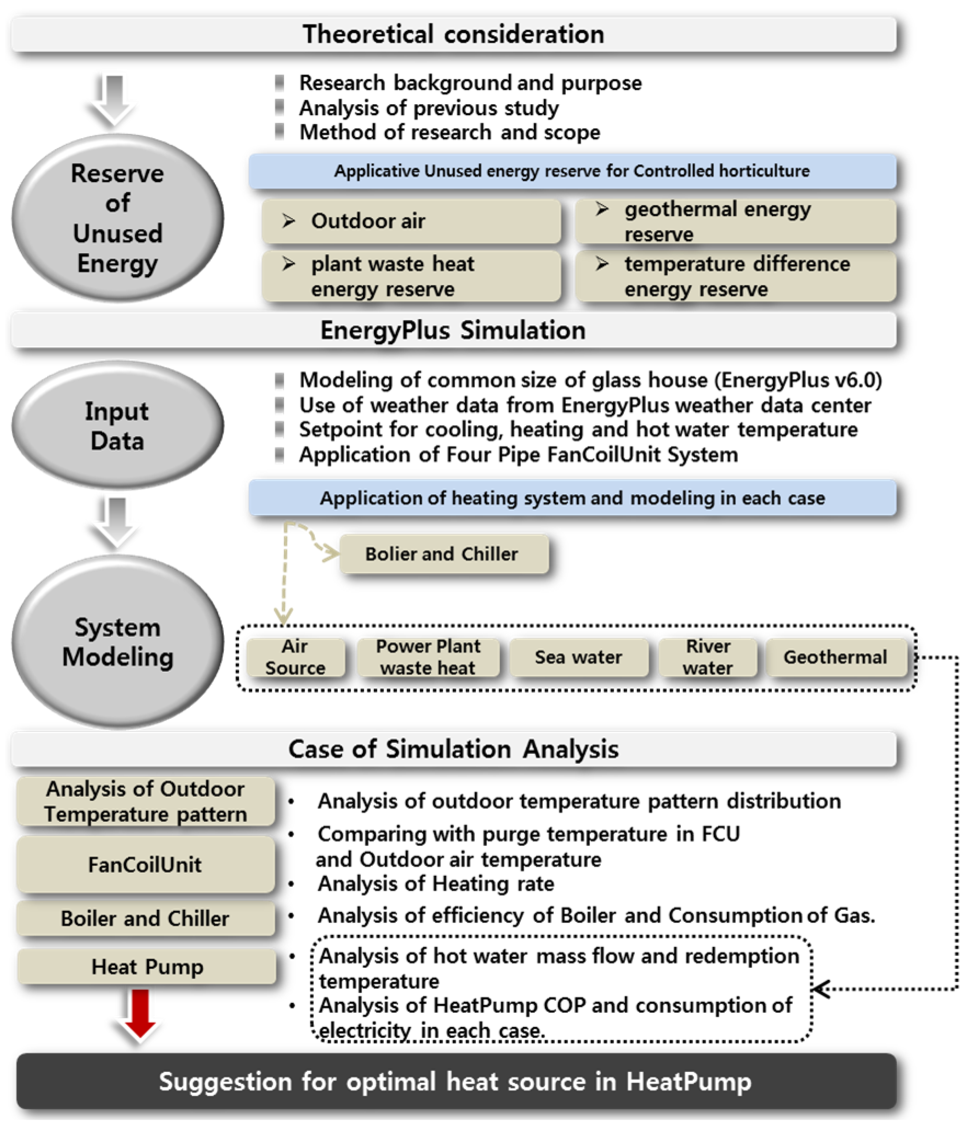
1.2. Methods and Scope

In this study, we performed modeling of a general sized large-scale glasshouse facility in Korea by using EnergyPlus with the goal of reducing heating energy consumption for horticulture by introducing new and renewable energy. We employed EnergyPlus version 6.0 and used the Incheon meteorological data provided by EnergyPlus. The heat sources applied to horticulture were air heat source, geothermal heat, power plant waste heat, sea water heat, and river water. In addition, the days in a year when the heating load is the highest were chosen as the representative days, and the indoor temperature at each time was set according to the culture conditions of tomato, which was the cultured plant chosen for this study [10]. Accordingly, the indoor flow-in rate through the Fan Coil Unit (FCU), the blowdown temperature, the return temperature, the COP performance, the boiler gas consumption, and the heat pump electricity consumption were analyzed for each case and compared with each other to suggest a heat pump for the optimum heat source to reduce the horticulture heating energy consumption. The study was conducted following the flow chart shown in Figure 1.
Figure 1. Study flow chart.
Energies 07 04781 g001

2. Unused Energy Reserves

2.1. Overview of Unused Energy Source Types

“Unused energy” refers to “recycled energy (waste heat from urban areas)” which is produced as a result of activities of humans or industries but discharged, not being effectively recollected, due to its economical value or limitations in utilization methods, and “temperature difference energy” which is one of natural energy sources abundant in nature and whose utilization does not have a significant ecological effect on the urban environment [8]. The temperature difference energy refers to sea water, river water, and lake water whose temperature is lower than the air in summer and higher than the air in winter and therefore they are used for heating and cooling or as hot water, taking advantage of the temperature difference. Utilization of the recycled energy refers to utilization of various waste heat sources discharged from industrial facilities such as waste incinerators, subways, wastewater treatment plants, electric power substations, and electric power plants for heating and cooling or as hot water [11]. Table 1 shows how the unused energy from each source is utilized [12,13].
Table 1. Utilization of unused energy.
SourceMediumUtilization MethodHeat Source Temperature Range (°C)
River waterwaterheat source for heat pump, cooling water0–10
Sea waterwaterheat source for heat pump, cooling water3–8
Groundwaterwaterheat source for heat pump, cooling water4–15
Wastewater plantraw wastewaterheat source for heat pump>10
treated waterheat source for heat pump
digestion gaspower generation and heat supply
sludgepower generation and heat supply
Waste incineratorhot gasheat recovery through vapor, power generation and heat supply15–30
hot water (condenser for power generation)heat source for heat pump, direct use
Atmosphereairheat source for heat pump−10–15
Exhaust airairheat source for heat pump15–25
Factories, etc.hot gasheat recovery through vapor power generation and heat supply10–80
hot waterheat source for heat pump, direct use
LNG thermal energypower generation, air liquefaction, etc.
Electric power plants (condenser)hot waterheat source for heat pump, utilization for culturing, etc.20–35

2.2. Definition of Unused Energy Reserve

To utilize unused energy, it is necessary to know the reserves of each unused energy source, but until now there has not been a clear definition of unused energy reserves. Reserves of temperature difference energy such as river water and sea water may be defined differently according to the utilization method. Since heat is supplied through a heat pump in this study, the temperature difference between the inlet and the outlet of a heat exchanger is the heat quantity which is actually available. Generally, the temperature difference between the inlet and outlet of a heat exchanger is about 3–5 °C, which may be considered as the energy reserve. In this study, therefore, the standards of estimating energy reserves for each heat source were set as a comprehensive concept, and the data described above were used as the basis for estimating the reserves of unused energy sources. In Japan, on the other hand, the reserves of unused energy sources are calculated by using Equation (1) [14,15,16,17,18]:
E = ΔtQC
where E: Energy reserve (kWh/month), Δt: Temperature difference (°C), Q: Flow rate (m3) and C: Specific heat (kWh/m3·°C).

2.3. Geothermal Energy Reserve

Geothermal energy is an important recycled energy which causes almost no environmental burden and is appropriate for taking charge of the base load. In general, geothermal energy is defined as the heat stored inside the Earth, referring to the energy including the heat included in the fluids in the rock mass and the pores (pore water). When geothermal power generation was the main concern in the past, geothermal energy was defined as the heat which may be extracted from the inside of the Earth. However, due to the recent explosive supply of the geothermal heat source heat pumps, the concept of geothermal energy includes not only heat extraction from the Earth’s interior but also discharge of heat to the ground as well as heat storage in the Earth. Therefore, the definition of geothermal energy is not extended to the heat stored in the solids or fluids contained in the Earth [19].
On the other hand, the factors used to estimate the geothermal energy reserve in Korea were density (ρ), specific heat (C) heat conductivity (K), ground surface heat (q0), ground surface heat productivity (A0), attenuation depth (b), volume (V), temperature at an arbitrary depth z (TZ), and ground surface temperature (T0), and the values of these factors are found in a domestic report in which the geothermal energy reserve in Korea was assessed [20]. In addition, with regard to the ground temperature which is necessary to assess the thermal energy reserve, the temperature was 23.9–47.9 °C at 1 km, 34.2–79.7 °C at 2 km, 44.2–110.9 °C at 3 km, 53.8–141.5 °C at 4 km, and 62.1–171.6 °C at 5 km [20]. Therefore, to estimate the final thermal energy reserve, we employed the volumetric method which is the most common method to calculate the energy included in a certain volume and the geothermal energy reserve. The total geothermal energy reserve (Q) in the entire Korea was calculated for each of 1 km depth interval from the ground surface to 5 km by using Equation (2) [21,22,23]:
Q = ρCPV(TZT0)
Table 2 shows the geothermal energy reserve calculated by Equation (2) for each depth interval from the ground surface to 5 km [20].
Table 2. Geothermal energy reserve in each depth interval.
Depth IntervalHeat Content in JHeat Content in GToeHeat Content in GToe (2%)
0–1 km4.25 × 1021101.12.0
0–2 km1.67 × 1022398.78.0
0–3 km3.72 × 1022884.917.7
0–4 km6.52 × 10221552.831.3
0–5 km1.01 × 10232396.047.9

2.4. Power Plant Hot Waste Water Reserve

Power plant hot waste water refers to the cooling water used at a thermoelectric power plant or a nuclear power plant in which vapor is condensed to water through a recycling perfusion system to absorb the electric power generation waste heat and the temperature of the water is increased by the waste heat. According to the hot waste water effluent standards for power plants in Korea, the maximum allowable temperature at the outlet is 35 °C and the temperature is usually 20 °C in winter and 35 °C in summer [2].
With regard to the power plant hot waste water reserve, the annual waste heat discarded from power plants in the form of hot waste water effluent was 388.0 TWh in 2008 [24]. The amount of energy used for greenhouse heating in a year is about 13.2 TWh which is just 3.4% of the waste heat, and the temperature distribution of the waste heat is also very appropriate as an energy source for greenhouse heating [25].
Table 3 shows the yearly power generation and the hot waste water effluent at each of the power plants located in Incheon which was the study subject region, indicating that the hot waste water reserve discharged from the thermoelectric power plants in Incheon is greater than the amount of energy consumed for greenhouse heating each year [26]. Therefore, it is possible to utilize the power plant hot waste water as a heat source for a large-scale horticulture complex.
Table 3. Yearly gross power generation and hot waste water outflow in Incheon.
Power StationYearly Gross Generation (TWh)Heated Effluent Outflow (×10−1 Billion Ton)
West coastWest Incheon8.84.6
Incheon0.32.2
New Incheon12.28.7
Posco Incheon2.41.9

2.5. Temperature Difference Energy Reserves

2.5.1. Sea Water Heat Energy Reserve

Generally, sea water heat energy reserve is estimated with sea water whose salinity is about 3.5‰ and the specific heat of the sea water is about 970 Mcal/m3 °C. In addition, although sea water reserves may be considered as infinite, the sea water flow rate used for heating and cooling may be assumed to be proportional to the effective coastal line length and can be expressed as Equation (3) [8,13,27]:
Q = (Effective coastal line length) × (Available flow rate per unit coastal line length)
In this study, with reference to the data obtained from the Kansai region in Japan, the sea water flow rate per unit coastal line length available for one month was defined as the total amount of sea water contained in the sea until the water depth of 10 m and the distance from the coast of 1 km. On the other hand, when the water depth was smaller than 10 m within 1 km distance from the coast, the sea water amount corresponding to the actual sea water depth was applied. When the coastline is severely crooked, an appropriate straight distance was set so that the minimum distance from the coast might be 1 km and then the effective coastal line length was calculated by using the straight distance [8,13,27].
The available temperature difference was determined as Δt = 1 °C considering the sea environment and referring to an international case [17]. According to the above definitions, the sea water heart energy reserve is defined as in Equation (4):
Energies 07 04781 i001
If the average water depth within 1 km of the distance from the coast is less than 10 m, the energy reserve is calculated by multiplying the ratio with reference to 10 m to Equation (4) as follows:
Energies 07 04781 i002
In addition, to obtain the sea water temperature data, the monthly average sea water surface temperature and the air temperature on the sea were investigated for the winter season (December to February) over ten years from 2003 to 2013 from the records of the Korea Hydrographic and Oceanographic Administration in the Incheon region corresponding to the Gyeonggi Bay, which is the subject region of this study. Figure 2 shows the monthly average sea water surface temperature and the air temperature on the sea obtained from the data [8,13,27].
Figure 2. Variation of the monthly average sea water surface temperature and the air temperature on the sea during winter over 10 years.
Energies 07 04781 g002
The investigation showed that during the winter season (December to February), the monthly average sea water surface temperature was 3.6 ± 3 °C and the monthly average air temperature on the sea was −0.8 ± 17 °C The daily variation of the sea water surface temperature was in the range of 0.4 ± 0.2 °C while that of the monthly average air temperature on the sea was in the range of −3.2 ± 3 °C Since the yearly sea water temperature variation was much smaller than that of the air temperature on the sea, a heat pump using sea water as a heat source may be operated under stable conditions [8,27].
To calculate the reserve, the effective coastal line length was investigated by using the navigation bibliography list including the coastal map published by the Korea Hydrographic and Oceanographic Administration in 1996. When calculating the effective coastal line length, the coastal line at the time of low tide was determined as the effective coastal line since the sea floor is shown during the time of low tide, and roughly calculated average water depth was determined as the effective coastal line for the coast of which water depth is less than 10 m [28]. Table 4 shows the effective coastal line length and the sea water heat energy reserve in Incheon region as investigated by the methods described above [8,13,27].
Table 4. Effective coastal line length and sea water heat energy reserve in Incheon region.
RegionEffective Coastal Line Length (km)Average Water Depth within 1 km Distance from the Coast (m)Reserve (Tcal/year)Available Heat Energy (Tcal/year)
Incheon Metropolitan City (Including Yeongjong Island)23.7 66.410 458444457

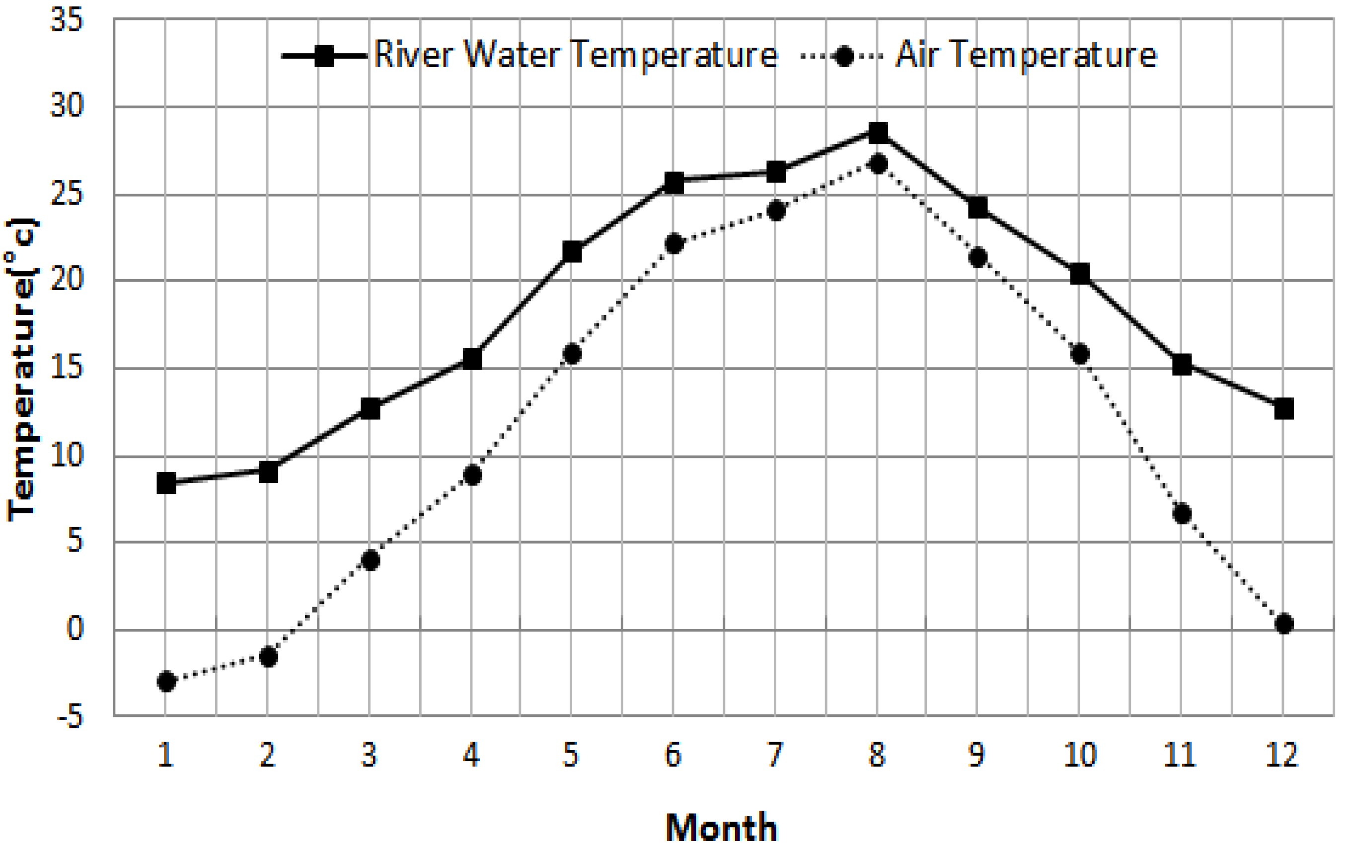
2.5.2. River Water Heat Energy Reserve

The river water heat energy reserve was calculated by using the method applied by NEDO (New Energy and Industrial Technology Development Organization), Japan, and the monthly average flow rate was used for the calculation because flow rate is highly dependent on the rainfall, basin area, geographic features, topography, and geological status [8,29]. Two types of available temperature difference were taken into account with regard to river water temperature difference: Δt is equal to the actual temperature difference, or Δt is constantly 5 °C. The specific heat was set to be 1000 Mcal/m3·°C. Figure 3 shows the monthly average temperature of the air and the river water throughout 2013 in Incheon region obtained from the Water Information System [8,13,27].
Figure 3. Monthly average temperature of air and river water throughout 2013 in Incheon region.
Energies 07 04781 g003
The calculation result showed that the unused river water energy reserve calculated with reference to the actual temperature difference between the air and the water was not very different from that calculated with reference to a constant temperature difference of Δt = 5 °C [8,27].
On the other hand, since the water level-flow rate curve which is generally used for water flow rate calculation includes a variety of uncertainties and thus causes an error in the calculated flow rate, highly reliable observance positions for each river where observance is performed each year were selected and the flow rate data at those positions were used to predict the flow rate of other positions in this study by a specific flow rate calculation method [8,27]. The calculated specific flow rates are found in detail in the investigated domestic reports about the temperature difference energy reserves. Table 5 shows the calculated river water heat energy reserve [8,13,27].
Table 5. River water energy reserve and available energy in each region.
RegionFlow Rate (m3/s)Reserve (Tcal/Year)Available Energy (Tcal/Year)
Seoul387.7160,485513
Incheon, Gyeonggi178.9228,318237
Total566.6388,803750

3. Methods

3.1. Simulation Software

A robust building energy simulation program, EnergyPlus version 6.0, was used for the simulations. EnergyPlus is a whole-building energy simulation program developed by DOE (The US Department of Energy) [30]. EnergyPlus was selected because it is a heat balance based simulation program and the heat balance method is the current industry standard method for calculating space loads [31]. Furthermore, one of the strong points of EnergyPlus is the integration of all aspects of the building simulation—loads, systems, and plants. System and plant output is allowed to directly impact the building thermal response rather than calculating all loads first, then simulating systems and plants. EnergyPlus is fully tested and validated against experimental data. For more information about the development and validation of the EnergyPlus program, see [32]. In this model, the amount of needed hot water supplied to the horticulture facility through fan coil unit (FCU) from the heat pump was calculated to compare the COP performance of the heat pump with each other. FCU is composed of water heating coil, water cooling coil and fan. In the heating mode, the heating coil utilizes hot water supplied from the central plant to produce the hot air. In the cooling mode, the cooling coil utilizes chilled water supplied from the central plant to produce the cold air.

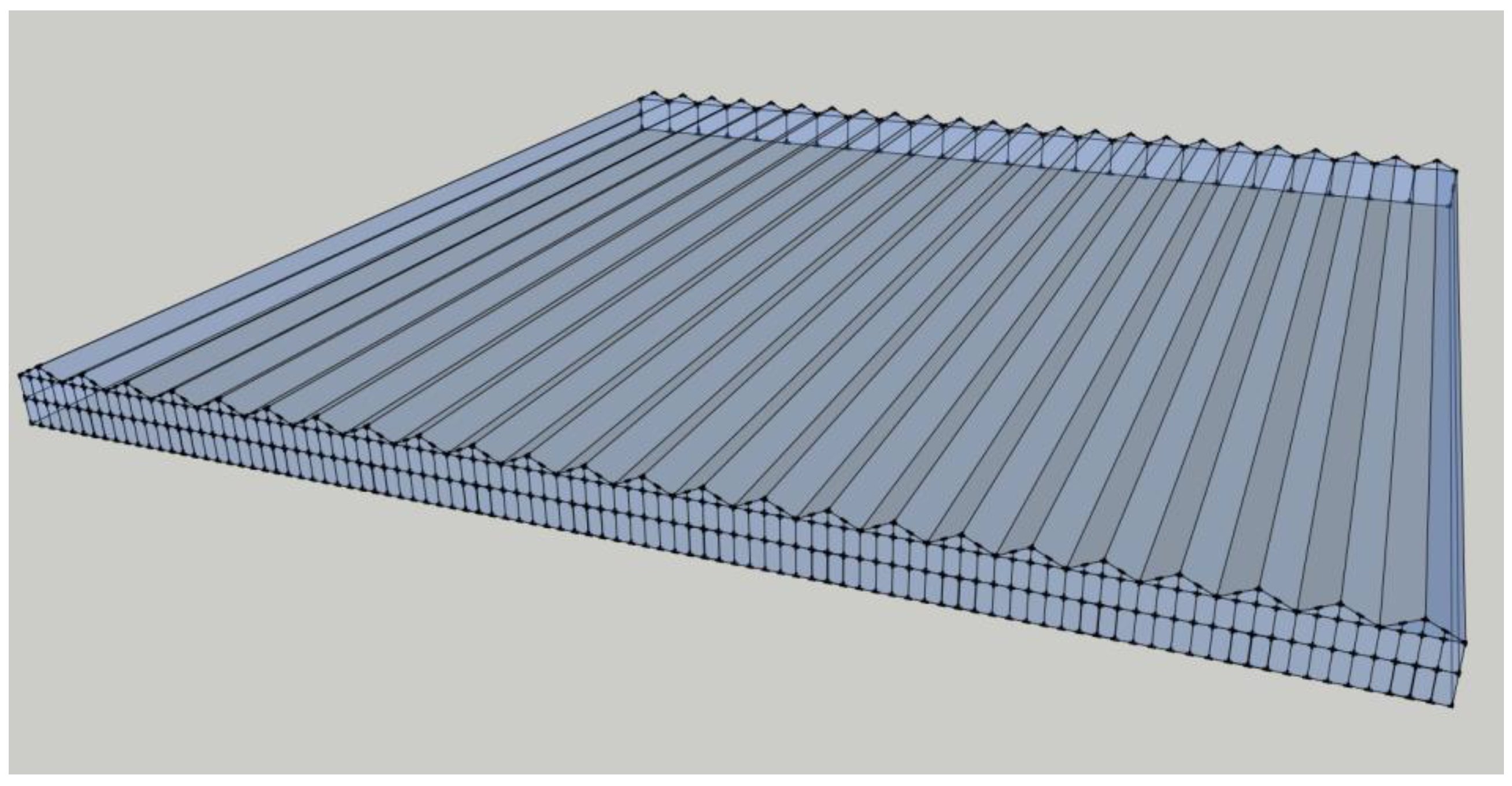
3.2. Description of the Simulated Greenhouse

Figure 4 shows the EnergyPlus simulation model. Within 100 ha horticulture facility modeled for this study, the detailed analysis was performed with a 100 m long and 100 m wide rectangular shape having an area of 1 ha (10,000 m2) which is a standard shape of a large-scale horticulture facility.
Table 6 shows the input physical properties of the iron frame [7].
Figure 4. Simulation model.
Energies 07 04781 g004
Table 6. The iron frame physical properties applied to the simulation.
PropertyInput Data
Width5.6 cm
Thermal conductivity58 W/m3
Density7850 kg/m3
Specific heat465 J/kgK

3.3. HVAC System, Ventilation Rate and Indoor Set-Points

The air infiltration rate applied to the glasshouse was 1.84 ACH (Air Change per Hour). This is an actual infiltration rate of a glasshouse measured by using a blower door instrument according to the pressure difference measurement method of ASTM E 779 [33] by Kim et al. [34]. Each greenhouse is served by a conventional fan coil unit (VAV) terminal unit. The EnergyPlus object ZoneHVAC:FourPipeFanCoil was used for the realistic modeling of fan coil unit [35]. The FCU is composed of a constant speed fan, hot water coil and chilled water coil. In the heating mode, the hot water is supplied from the central plant and its flow rate is modulated to adjust the air discharge temperature from FCU. Similarly, in the cooling mode, the chilled is supplied and its flow rate is modulated to meet the cooling load in the greenhouse. The entering chilled/hot water temperatures for cooling/heating were set to be 7.0 °C and 40.0 °C, respectively. HVAC (heating, ventilating and air-conditioning) systems operate 24 h every day during the whole year. The indoor air temperature set-points during night-time and day-time were set at 11 °C and 23 °C, respectively, which is known to be the proper conditions for tomatoes. EnergyPlus uses an iteration method over the entire HVAC system in order to converge the system controllers based on the set-point [25]. The iteration proceeds and the system controllers are simulated in sequence until the calculated indoor temperature value in each thermal zone matches the set-point within the specified tolerance. The controllers are converged by the method of interval halving, which was chosen for its robustness [36].

3.4. Plant Modeling

As stated in the previous sub-section, six cases were simulated. The differences among the simulated cases lie in way how chilled water and hot water are produced. Case 1 uses chiller and boiler to produce the chilled and hot waters, while Case 2–Case 6 use heat pumps. In Case 1, it was assumed that the temperature of the fluid entering the source side of the chiller after being produced by the cooling tower, Tef in the equation below, is 3 °C higher than the outdoor wet-bulb temperature. Chiller and boiler curves are expressed in the following equations:
For PLR < 0.0667, E f fBR = 15 × PLR × E f fNom For 0.0667 ≤ PLR, E f fBR = E f fNom
Energies 07 04781 i003
where PLR is boiler part load ratio, EffBR is boiler thermal efficiency, Effnom is nominal boiler thermal efficiency, COPCH is chiller COP, COPref is reference chiller COP, Tcw is the chilled water leaving temperature, Tef is the condenser fluid entering temperature. a~f are the performance curves for the chiller, which are based on the catalog data. a is 0.4953775, b is −0.0135934, c is 0.0005784637, d is 0.02778142, e is 0.0001747259 and f is −0.0008590768.
The performance of the heat pump was calculated from the Pressure-Enthalpy graph and refrigeration cycle of the refrigerants, with load-side temperature of 7–12 °C when cooling and 40–45 °C when heating. The following COP curve was used to determine the heat pump COP as a function of the different heat source temperatures:
Energies 07 04781 i004
where, ΔT is the difference between the return and entering water temperatures in, TEF is entering fluid temperature (°C) and COPHP is heat pump COP. In Case 6, it was assumed that there is sufficient separation between the pumping site and return site for the groundwater temperature and that the groundwater temperature is equal to the annual average ambient air temperature over the year [37,38].

3.5. Simulated Cases

Six cases were studied. All six cases are identical in terms of the terminal unit in that FCUs are operated to meet the heating and cooling load in the greenhouse. The differences among the simulated cases lie in way how chilled water and hot water are produced. The baseline case is Case 1 in which the chilled water and hot water to be supplied into FCUs are produced by the gas-fired boiler and the centrifugal chiller. Case 1 represents the conventional system used in practice. Case 2 employs the air-source heat pump in which the outdoor air is the heat source. Case 3 utilizes the heat pump with the heat source of waste water from the power plant. As discussed in the previous Section 2, the temperature of the waste water entering the source side of the heat pump is assumed to be 25 °C during the whole year. Case 4 and Case 5 utilize the heat pump with the heat source of sear water and river, respectively. The monthly variations of the sea water and river temperature are provided in Section 2. Finally, Case 6 employs a ground source heat pump, where a groundwater heat pump (GWHP) using the groundwater as a heat source is considered. The simulated cases are summarized in Table 7.
Table 7. Simulated cases.
CaseTerminal Unit at GreenhouseHeating/Cooling EquipmentHeat Source
1Fan coil unitBoiler/Centrifugal chillerN.A.
2Fan coil unitHeat pumpOutdoor air (aerothermal energy)
3Fan coil unitHeat pumpWaste water from power plant
4Fan coil unitHeat pumpSea water (hydrothermal energy)
5Fan coil unitHeat pumpRiver (hydrothermal energy)
6Fan coil unitHeat pumpGroundwater (geothermal energy)

4. Simulation Analysis

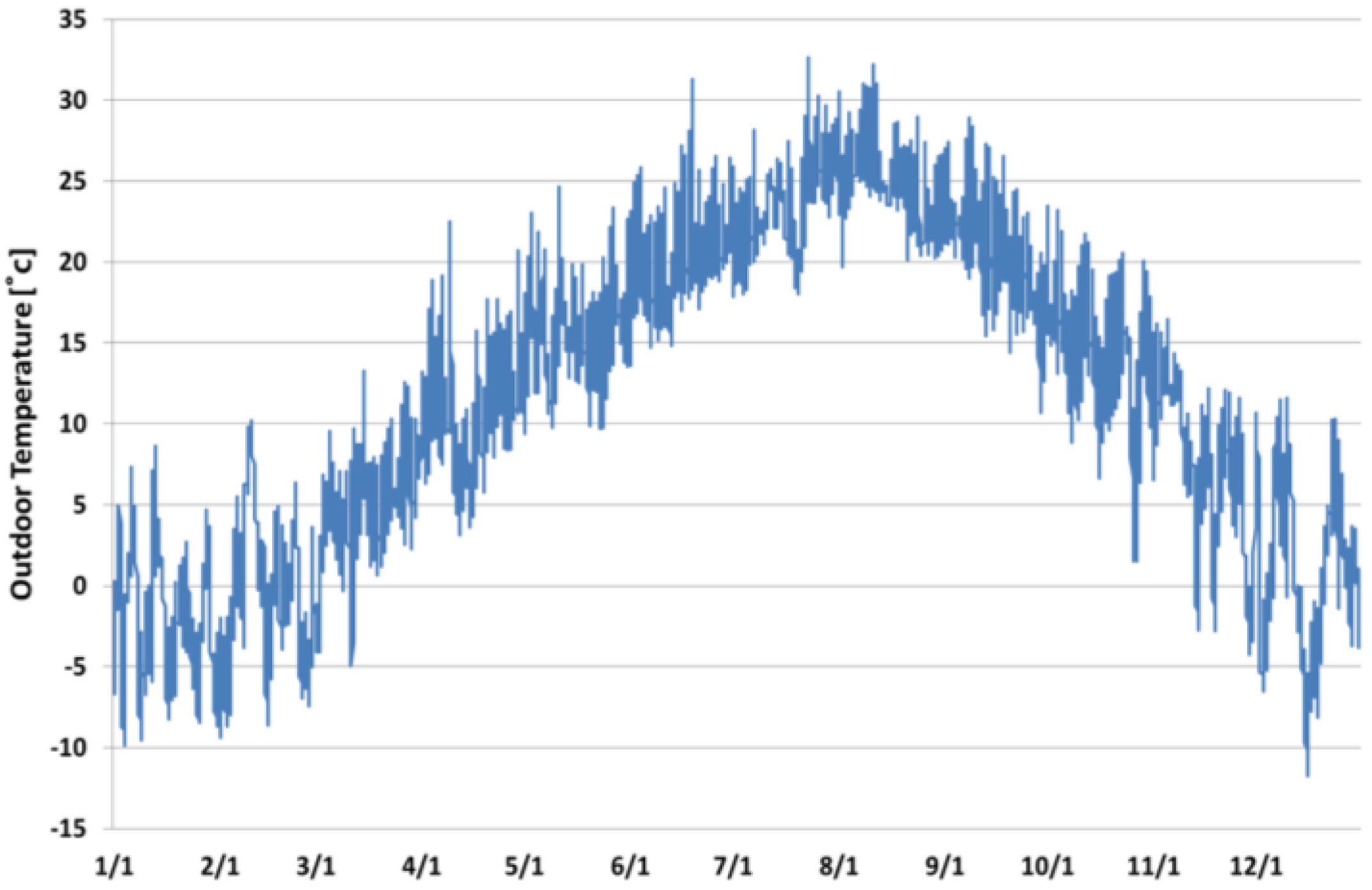
4.1. Analysis of Outdoor Air Temperature

Figure 5 shows the outdoor air temperature in Incheon over a year. Incheon is located at latitude 37°48'N and longitude 126°55'E, and the meteorological data provided by EnergyPlus were used in this study. The analytical result showed that the yearly average outdoor air temperature was 11.9 °C. The yearly lowest air temperature was −9.7 °C on 15 December, while the yearly highest air temperature was 32.6 °C on 23 July. The winter season (January, February, and December) was taken into consideration in this study, and the air temperature was in the range of −10 ~ 10 °C with the average air temperature of −0.42 °C. For the analysis, the coldest day in a year, which was 15 December, was used as the representative day in which the temperature was in the range −3.9 ~ –9.7 °C.
Figure 5. Outdoor air temperature of Incheon City.
Energies 07 04781 g005

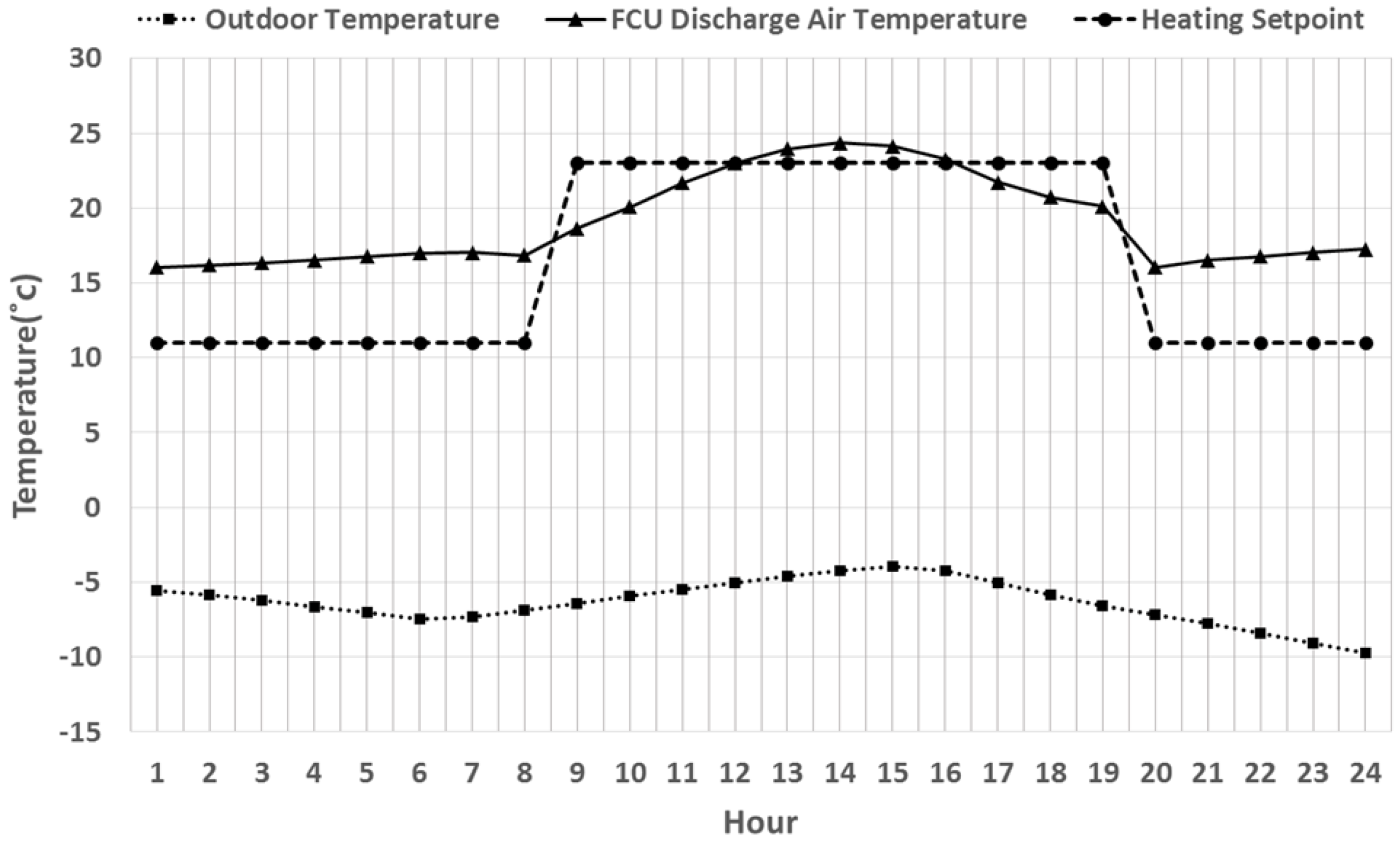
4.2. Comparative Analysis of FCU Air Discharge Temperature and the Outdoor Air Temperature

In this study, 15 December, the coldest day in a year, was chosen as the representative day for the analysis. Figure 6 shows the temperature of the air discharged from the FCU and supplied to the inside of the horticulture facility as well as the outdoor air temperature. The temperature of the air discharged from FCU and supplied to the inside of the horticulture facility was in the range 16.1–24.3 °C Since the setup indoor temperature was 11 °C from 19:00 to 9:00 and 23 °C from 9:00 to 19:00, the FCU air discharge temperature might have showed a pattern similar to that of the indoor setup temperature. As shown in the figure, the discharge air temperature of the FCU is approximately 5 °C higher than the indoor heating set-point. Based on the nature of FCUs, the air flow is constant regardless of the load variation and thus the discharge air temperature is controlled to meet the heating load. Therefore, the discharge temperature showed the similar pattern to the heating set-point variation as shown in the figure.
Figure 6. FCU discharge air and outdoor air temperature variations.
Energies 07 04781 g006

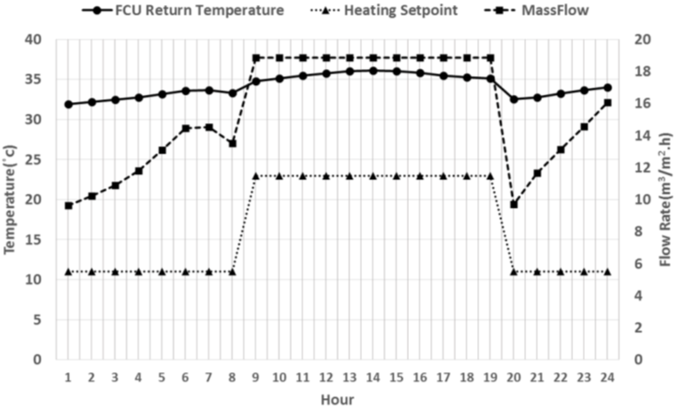
4.3. Analysis Return Water Temperature through FCU and Hot Water Flow Rate

Figure 7 shows the analyzed return water temperature through FCU and the hot water flow rate per unit area in each hour. As mentioned previously, the hot water temperature supplied to the FCU was set to be 40 °C throughout the year. The temperature of the hot water returned after heat exchange in the FCU was in the range of 31.9–36.1 °C. The heating set point from 19:00 to 9:00 was 11 °C which was lower than the heating set point from 9:00 to 19:00, 23 °C, and thus the air temperature returning to the FCU was also low. In addition, heat was lost through the glass, the covering of the glasshouse, during the night hours, and thus more heat was taken from the hot water supplied at 40 °C in order to reach the set point. That may be the reason why the temperature of the return hot water is lower during the night hours than that during the day hours. On the contrary, the heating set point for the day hours was higher than that for the night hours, but heat was obtained from the glass covering and thus the temperature of the air returned to the FCU might have been higher during the daytime. Therefore, even though the temperature of the supplied hot water was the same as 40 °C during both the night and the day, more heat was taken by the air during the daytime and thus the returned water temperature was higher during the daytime than that during the nighttime. The pattern of the hot water flow rate per unit area was also similar to that of the returned water temperature. The hot water flow rate per unit area was the highest as 18.8 m3/m2·h during the time interval from 9:00 to 19:00 and the lowest as 9.6 m3/m2·h at 1:00. The flow rate may be varied by the indoor temperature set point. Therefore, the difference between the indoor temperature setpoint and the supplied hot water temperature (40 °C) causes the flow rate to vary. When the indoor temperature setpoint is decreased, the difference between the indoor temperature setpoint and the supplied hot water temperature is increased. When the indoor temperature setpoint is decreased, the supplied hot air temperature also decreases, so the flow rate is thereby decreased. Since the indoor temperature setpoint is higher during the daytime than that during the night time, the difference between the indoor temperature setpoint and the supplied hot water temperature is smaller and the supplied hot air temperature higher, so hot water transfers more heat to the air during the daytime than during the night time in the FCU. Thus the flow rate during the daytime is higher than that during the night time. In addition, as the flow rate is varied, the return water temperature during the night time also is lowered by the decreased flow rate, which may be the result of the FCU control method of EnergyPlus.
Figure 7. FCU hot water supply flow rate and return water temperature.
Energies 07 04781 g007

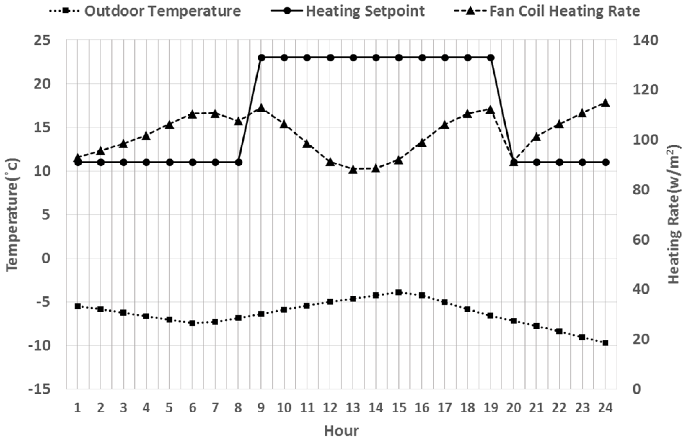
4.4. Analysis of Heat Flow Rate Supplied to the FCU

Figure 8 shows the heat quantity per unit area supplied to the FCU, the outdoor air temperature, and the indoor temperature set point. The heat quantity per unit area supplied to the FCU may be analyzed by dividing time into two intervals, as in the analysis described above. The first time interval is from 19:00 to 9:00 when the temperature setpoint is low and heat is taken away externally. The second time interval is from 9:00 to 19:00 when the temperature setpoint is high and heat flows internally from the sunlight. In the first time interval from 19:00 to 9:00 when the temperature set point is low, the heat quantity supplied to the FCU was increased as the indoor temperature setpoint was decreased. The heat quantity was temporarily increased at 9:00 as the indoor temperature setpoint shifted from 11 °C to 23 °C However, as the sunlight started to be introduced to the interior, the indoor air temperature was increased. As a result, the heat quantity was decreased until 13:00 and then increased after 13:00 when the sunlight started to decrease. The heat quantity was also decreased from 20:00 as the indoor temperature set point was decreased. Afterward, the heat quantity was increased. This might be because the heat loss through the glass was increased as the outdoor air temperature was decreased, and the heat quantity was increased to maintain the indoor temperature set point. The heat quantity was the lowest as 92.01 W/m2 at 15:00 when the outdoor air temperature was the highest, while the heat quantity was the highest as 114.93 W/m2 at 24:00 when the outdoor air temperature was the lowest.
Figure 8. FCU supply heating rate variations.
Energies 07 04781 g008

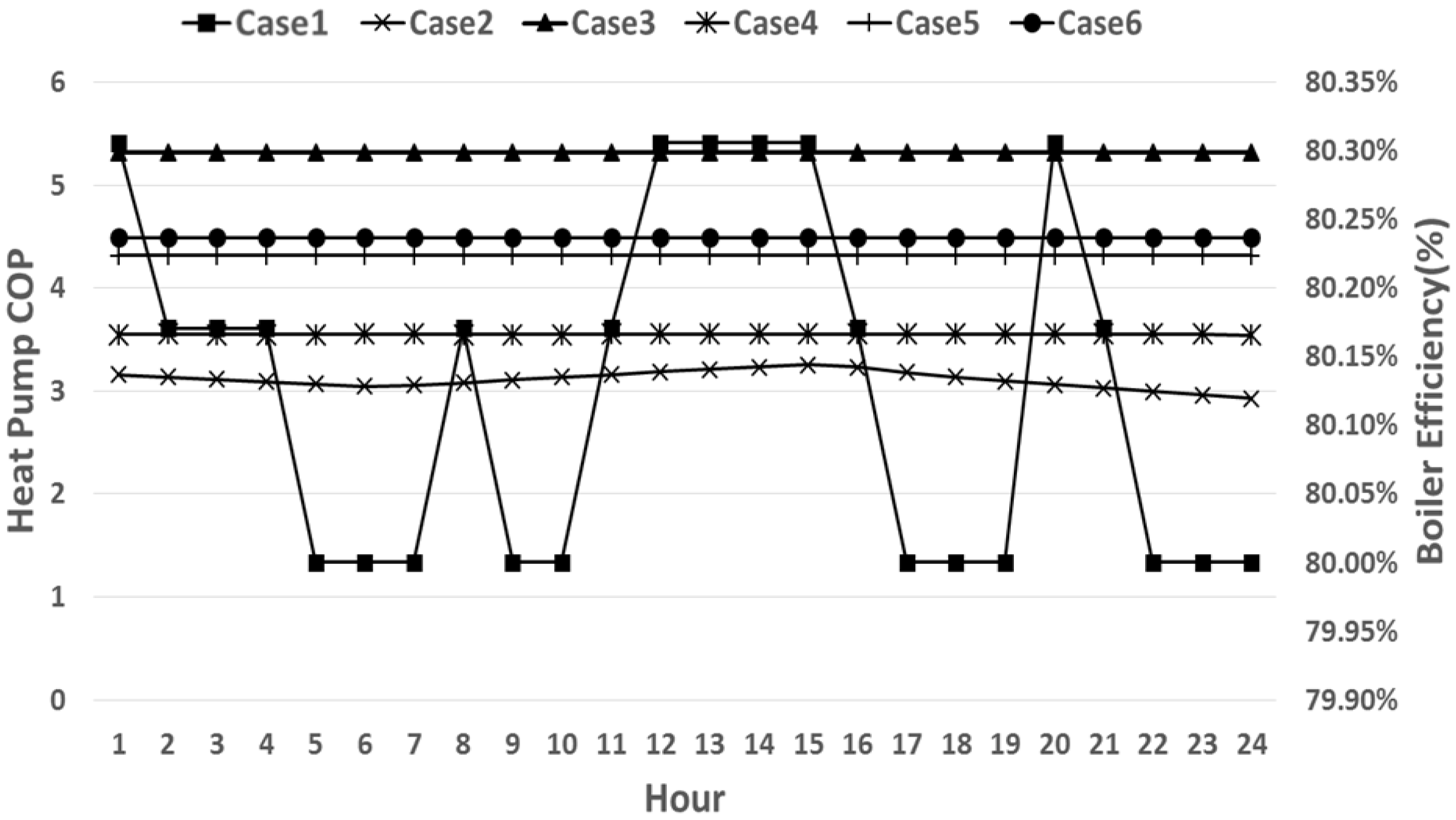
4.5. Heat Pump COP and Boiler Efficiency of Each Heat Source

Figure 9 shows the heat pump COP and boiler efficiency of each heat source. The Cases 1–6 shown in Figure 9 were previously described in Table 3. The input heat source temperature was the temperature mentioned in Section 2.2. The outdoor air temperature was the meteorological input data for the simulation. Case 1 was a base model without a heat pump but with a boiler, and thus the boiler efficiency was calculated. In the other five cases, the heat pump COP was calculated. In Case 1 base model, the boiler efficiency was mostly 80%. Although the efficiency was increased by up to 0.3% in the time intervals between 0:00 and 4:00 and between 10:00 and 17:00, the increased was insignificant. Thus, it may be assumed that the efficiency of 80% was maintained all the time for 24 h. In this study, Equation (1) was employed to calculate the boiler efficiency variation by the partial load rate. Since the efficiency was 80% or higher over the entire time range, it is presumed that the boiler was mostly operated under a high partial load rate condition. In Cases 2 to 5 in which a heat pump was used, the COP was the highest as 5.31 when power plant waste heat was used as a heat source. The COP was 4.49 when geothermal heat was used as a heat source and 4.31 when river water used as a heat source. The COP was relatively low as 3.55 when sea water heat was used and as 3.16 when outdoor air was used. The COP was greatly dependent on the temperature of the heat source: the heat pump COP was higher as the heat source temperature was higher.
Figure 9. Boiler efficiency and heat pump COP variations.
Energies 07 04781 g009

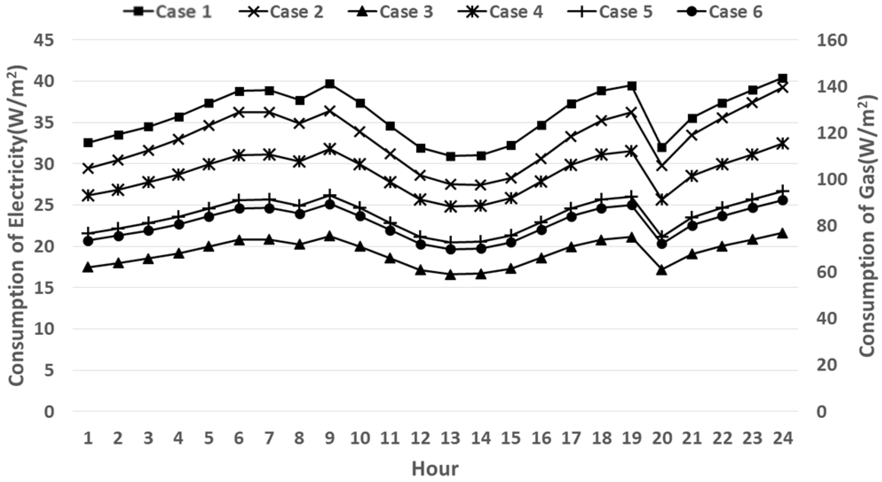
4.6. Comparative Analysis of Gas and Electricity Consumption for Each Heat Source

Figure 10 shows the gas and electricity consumption. As mentioned above, gas consumption occurred in Case 1 where a boiler, instead of a heat pump, was used. Electricity consumption was shown in other cases. The large-scale glasshouse in our analysis has a large area of 100 m × 100 m and thus the energy consumption was very high. Therefore, energy consumption per unit area was calculated for the analysis by dividing the energy consumption by the glass house area. The energy consumption pattern was similar for all the cases. As mentioned in Figure 8, as the outdoor air temperature was decreased from 0:00 to 6:00, the heating rate was increased and the gas/electricity consumption was increased accordingly in all the cases. In the time interval from 9:00 to 18:00, the energy consumption was decreased and then increased at about 14:00 due to the increased outdoor air temperature and the sunlight obtained through the glass. After 20:00, as the outdoor air temperature was decreased, heat loss through the glass was increased and the gas/electricity consumption was increased accordingly in proportion to the increased heat quantity. The lowest gas/electricity consumption was found at 14:00 in a day when much heat was obtained through the glass and the outdoor air temperature was high. In Case 1, the maximum gas consumption 143.66 W/m2, which was 6.6 times higher than the electricity consumption in other cases. Among the cases where a heat pump was used, Case 3 where the power plant waste heat having the highest heat pump COP, as shown in Figure 9 above, was used as the heat source showed that lowest electricity consumption. Case 2 where outdoor air was used as a heat source showed the highest electricity consumption. The electricity consumption was in the reverse order of the heat pump COP. The electricity consumption in Case 2, which was the highest among the cases, was 63.3 to 81.5% higher than that of Case 3 which had the lowest electricity consumption. It was once again confirmed that the heat source temperature has a great effect on the heat pump COP, which has a direction effect on the energy consumption in horticulture facility.
Figure 10. Hourly boiler gas and heat pump electricity consumptions.
Energies 07 04781 g010

4.7. Comparative Analysis of Gas and Electricity Consumption in Each Month

Table 8 summarizes the monthly total gas/electricity consumption during January, February, and December in each case. In all the analyzed data, the monthly total gas/electricity consumption was the lowest in February and the highest in January, except the case where sea water heat was used.
Table 8. Monthly total boiler gas and heat pump electricity consumptions.
CaseJanuary (kWh/m2)February (kWh/m2)December (kWh/m2)
Case 174.853.163.3
Case 218.012.514.5
Case 311.37.99.5
Case 416.711.712.7
Case 513.99.89.4
Case 613.49.411.3
The energy consumption was lowest in February not only because the number of days in the month is just 28, smaller than that of other months, but also because the outdoor air temperature was higher than in other months. The heat quantity needed in the case where sea water heat was used was lower in March than in January and February because the sea heat temperature was the highest in March. Therefore, in the case where sea water heat was used, the electricity consumption was the lowest in March. Analysis of the cases showed that the energy consumption was the lowest in the case where the power plant waste heat was used, as in the pattern found with respect to the winter representative days, and that the energy consumption was relatively low in the cases where geothermal heat and river water were used as a heat source. The heat pump energy consumption was relatively high in the cases where outdoor air and sea water heat were used as a heat source. The boiler gas consumption was the highest. Except for Case 1 where gas was used, the energy consumption in Case 3, having the lowest energy consumption, was 34.3% to 37.4% lower than that of Case 2, having the highest energy consumption. As in the previous analysis, such an energy consumption pattern might be the result of the temperature difference of the heat source supplied to the heat pump. The data showed that the energy efficiency of the heat pump using power plant waste heat as a heat source of which temperature was the highest was the highest.

5. Conclusions

In this study, a modeling of a large-scale horticulture facility was performed through EnergyPlus to compare the gas/electricity consumption for each case where unused energy is used as a heat source. The unused energy heat sources analyzed in this study were air source, power plant waste heat, sea water, river, and geothermal heat. A general gas boiler was employed as a baseline case for the analysis. The conclusions of this study are as follows:
  • The subject region of this study was the Incheon region of Korea where the yearly average air temperature was 11.9 °C The coldest day in a year was chosen as the representative day for the analysis. The temperature flowing into the greenhouse from the FCU was in the range of 16.1–24.4 °C. The indoor temperature set point in the greenhouse was 11 °C from 0:00 to 8:00, 23 °C from 9:00 to 19:00, and 11 °C from 20:00 to 24:00. The pattern of the indoor temperature setpoint was similar to that of the temperature of the air flowing into the greenhouse.
  • The hot water flow rate to the FCU was dependent on the indoor temperature setpoint and the supplied hot water temperature. Since the temperature of the supplied hot water was constant at 40 °C, the hot water flow rate was dependent on the indoor temperature setpoint. Therefore, the flow rate was high during the daytime when the indoor temperature setpoint was high, and the flow rate pattern was similar to the outdoor air temperature variation pattern during the night time. This may be because much heat was lost through the glass when the outdoor air temperature was low. Since the returned hot water temperature after heat exchange was varied by the flow rate, the returned hot water temperature variation pattern was similar to that of the flow rate.
  • The heat flow rate supplied to the FCU was higher when the outdoor air temperature was lower, since heat loss through the glass was increased during the night time although the indoor temperature setpoint was low. During the daytime, despite the higher indoor temperature setpoint, heat was acquired through the glass and thus the required heat quantity was lower than that during the night time. The supplied heat quantity was the lowest as 92 W/m2 at 15:00 when the sunlight was the highest and the outdoor air temperature was the highest during a day, while it was the highest as 114.9 W/m2 at 24:00 when the outdoor air temperature was the lowest during a day.
  • The heat pump COP pattern followed the temperature of the analyzed heat sources: the heat pump COP was the highest in the case where power plant waste heat, having the highest temperature, followed by geothermal heat, river water, sea water heat, and outdoor air. The efficiency of the gas boiler, which was the baseline case, was about 80%. The electricity consumption in the case where power plant waste heat was used as a heat source, which had the highest heat source temperature among the cases, was 63.3% to 81.5% lower than that of the case where outdoor air was used as a heat source. The monthly total gas/electricity consumption during January, February, and December when heating was performed was the lowest in the case where power plant waste heat was used as a heat source, as in the energy consumption pattern analyzed above.
Horticulture facilities of which covering is mostly glass require more heating energy than that of general buildings. In addition, horticulture requires heating even during the night, so more heating energy is necessary for a horticulture facility. This study is aiming at development of an energy supply and operation system utilizing unused energy sources for a large-scale horticulture facility. We applied a heat pump using unused energy sources as a heat source, derived the optimum heat source, and investigated the minimum gas/electricity consumption required for heating. On the basis of the results of this study, future studies will be conducted on energy supply systems using other industrial waste heat sources to investigate the feasibility of each system and to develop an operating system. Another improvement can be the economic analysis such as life cycle cost (LCC) assessment taking into account both the initial and operating cost.

Acknowledgments

This work was carried out with the support of “Cooperative Research Program for Agriculture Science & Technology Development (Project Title: Development of Optimal District Energy and Operation System using Industrial Waste Heat for Large-scale Horticulture Facility Applications, Project No: PJ01002101)”, Rural Development Administration, Suwon, Gyeonggi-do, Korea.

Author Contributions

All authors contributed equally to this work. All authors designed the simulations, discussed the results and implications and commented on the manuscript at all stages. In Tak Hyun performed the energy simulations and Yeo Beom Yoon led the development of the paper. Jae Ho Lee and Kwang Ho Lee performed the result analysis and discussion. Yu Jin Nam conducted detailed heat pump modeling.

Conflicts of Interest

The authors declare no conflict of interest.

References

  1. Heo, T. On the Application of the Heat Pump System to Facility Horticulture, Using Hot Waste Water from Power Plants. Ph.D. Thesis, Jeju National University, Jeju, Korea, February 2012. [Google Scholar]
  2. Yu, Y.S. Development of Greenhouse Cooling & Heating System Using Waste Heat of Thermal Generation Plant; Project No. PJ007432; National Academy of Agricultural Science: Suwon, Korea, 2012. [Google Scholar]
  3. Ryu, Y.S.; Joo, H.J.; Kim, J.W.; Park, M.R. Economic analysis of cooling-heating system using ground source heat in horticultural greenhouse. J. Korean Sol. Energy Soc. (KSES) 2012, 32, 60–67. [Google Scholar] [CrossRef]
  4. Park, Y.J. A Study on Field Test of the Horizontal Ground Source Heat Pump System for Greenhouse; 2005-N-GE-P-01; Ministry of Commerce, Industry and Energy (MOTIE): Sejong, Korea, 2007. [Google Scholar]
  5. Kim, J.S. Efficiency Analysis of Geothermal Heating and Cooling System Using Groundwater for Controlled Horticulture. Ph.D. Thesis, Andong University, Andong, Korea, August 2013. [Google Scholar]
  6. Baek, Y.J.; Lee, S.H.; Kim, M.S.; Lee, Y.S.; Jang, G.C.; Na, H.S. A simulation study on the annual heating performance of a seawater-source heat pump and air-source heat pump. In Proceedings of the Autumn Conference of the Korean Solar Energy Society (KSES), Seoul, Korea, 1–2 November 2012.
  7. Fabrizio, E. Energy reduction measures in agricultural greenhouses heating: Envelope, system and solar energy collection. Energy Build. 2012, 53, 57–63. [Google Scholar] [CrossRef]
  8. Park, J.T.; Jang, G.C. An investigation on quantity of unused energy using temperature difference energy as heat source and its availability. Energy Eng. J. 2002, 11, 106–113. [Google Scholar]
  9. Moon, J.P. Utilization of river bank filtration for horticulture facility. Korea J. Geotherm. Energy (KSGEE) 2012, 8, 10–14. [Google Scholar]
  10. Guidance on Energy Efficient Farm Product Management in Greenhouses; Rural Development Administration (RDA): Suwon, Korea, 2011; pp. 2–3.
  11. Jin, S.H.; Hong, E.J. The Feasibility Analysis of Urban Unused Energy: Focusing on Technology, Institution and Infrastructure; Korea Institute of Ecological Architecture and Environment (KIEAE): Seoul, Korea, 2013. [Google Scholar]
  12. Jeon, N.S. Guidance for Gyeong Nam Horticulture Facility in the Era of Low Carbon Green Growth; GyeongNam Development Institute: Changwon, Korea, 2009. [Google Scholar]
  13. Park, J.T.; Jang, G.C. Technology for Utilizing Unused Energy Sources. Korean Assoc. Air Cond. Refrig. Sanit. Eng. (KARSE) 2002, 19, 33–42. [Google Scholar]
  14. Unused Energy Resources for 21st Century; Department of Economy and Industry of Japan: Tokyo, Japan, 1990.
  15. Takeshi, K.; Hiroo, T.; Hisashi, M. Possibility of Utilization of River Water as the Heat Source/Sink of Heat-Pump Systems: Part I. In Proceedings of the Annual Conference of Architectural Institute of Japan, Tokyo, Japan, 12–14 September 1993; pp. 499–500.
  16. Hisashi, M.; Hiroo, T.; Takeshi, K. Possibility of Utilization of River Water as the Heat Source/Sink of Heat-Pump Systems: Part II. In Proceedings of the Annual Conference of Architectural Institute of Japan, Tokyo, Japan, 12–14 September 1993; pp. 501–503.
  17. Recent Advancement of Unused Energy Resources; Committee of District Energy of Renewable Energy Foundation: Tokyo, Japan, 1992.
  18. Utilization of Urban Gas for Unused Energy Source Applications; Unused Energy Sources Committee of Japanese Gas Association: Tokyo, Japan, 1991.
  19. Song, Y.H.; Kim, H.C.; Lee, Y.M.; Lee, T.J. Potential of geothermal energy in Korean peninsula. Soc. Air Cond. Refrig. Eng. Korea (SAREK) 2009, 38, 42–50. [Google Scholar]
  20. Park, S.H. Geothermal Resource Assessment in Korea. Master’s Thesis, Kongju University, Kongju, Korea, August 2008. [Google Scholar]
  21. Blackwell, D.D.; Negraru, P.T.; Richards, M.C. Assessment of the enhanced geothermal system resource base of the United States. Nat. Resour. Res. 2007, 15, 283–308. [Google Scholar] [CrossRef]
  22. Muffler, P.; Cataldi, R. Methods for regional assessment of geothermal resources. Geothermics 1978, 7, 53–89. [Google Scholar] [CrossRef]
  23. Tester, J.W.; Anderson, B.; Batchelor, A.; Blackwell, D.; DiPippo, R.; Drake, E.; Garnish, J.; Livesay, B.; Moore, M.C.; Nichols, K.; et al. The Future of Geothermal Energy: Impact of Enhanced Geothermal Systems (EGS) on the United States in the 21st Century; DOE Contract DE-AC07–05ID 14517 Final Report; Massachusetts Institute of Technology: Cambridge, MA, USA, 2006. [Google Scholar]
  24. Jo, J.H.; Kim, D.Y.; Lee, J.S. Directions for Developing Green Aquaculture Using Thermal Effluent from Power Plant; Korea Maritime Institute: Seoul, Korea, 2010. [Google Scholar]
  25. Yu, Y.S. Heat exchanger design of a heat pump system using the heated effluent of thermal power generation plant as a heat source for greenhouse heating. J. Bio-Environ. Control (KSBEC) 2012, 21, 372–378. [Google Scholar] [CrossRef]
  26. Electric Power Statistics Information System (EPSIS). Available online: https://epsis.kpx.or.kr (accessed on 28 February 2014).
  27. Lee, J.H.; Hyun, I.T.; Yoon, Y.B.; Lee, K.H. Investigation of Reserves and Potentials of Unused Energy Sources for Large-scale Horticulture Facility Applications. In Proceedings of the Summer Conference of the Society of Air-conditioning and Refrigerating Engineers of Korea, Yong Pyong, Korea, 25–27 June 2014.
  28. List of Publication of Nautical Charts and Documents; Korea Hydrographic and Oceanographic and Administration: Seoul, Korea, 1996.
  29. Park, I.H.; Yoon, H.; Park, J.T.; Jang, K.C.; Lee, Y.S. A study on the potential energy reserve amount of domestic river water as unutilized energy resource. Soc. Air-Cond. Refrig. Eng. Korea (SAREK) 2005, 17, 521–528. [Google Scholar]
  30. Crawley, D.B.; Lawrie, L.K.; Winkelmann, F.C.; Buhl, W.F.; Huang, H.J.; Pedersen, C.O.; Strand, R.K.; Liesen, R.J.; Fisher, D.E.; Witte, M.J.; et al. EnergyPlus: Creating a new-generation building energy simulation program. Energy Build. 2001, 33, 319–331. [Google Scholar] [CrossRef]
  31. ASHRAE Fundamentals Handbook; American Society of Heating, Refrigerating and Air-Conditioning Engineers, Inc.: Atlanta, GA, USA, 2009.
  32. EnergyPlus. Testing and Validation. Available online: http://apps1.eere.energy.gov/buildings/energyplus/testing.cfm (accessed on 28 February 2014).
  33. Standard Test Method for Determining Air Leakage Rate by Fan Pressurization; Active Standard No. ASTM E 779–87; American Society for Testing and Materials (ASTM): West Conshohocken, PA, USA, 1987.
  34. Kim, K.S.; Yoon, J.H.; Song, I.C. Energy performance evaluation of heat reflective radiant barrier systems for greenhouse night insulation. Archit. Inst. Korea (AIK) 2000, 16, 153–161. [Google Scholar]
  35. The USA DOE, 2012. EnergyPlus Input Output Reference. The Encyclopedic Reference to EnergyPlus Input and Output. Available online: http://apps1.eere.energy.gov/buildings/energyplus/pdfs/inputoutputreference.pdf (accessed on 28 April 2014).
  36. EnergyPlus, 2014. EnergyPlus Engineering Reference. The Reference to EnergyPlus Calculations. Available online: http://apps1.eere.energy.gov/buildings/energyplus/pdfs/engineeringreference.pdf (accessed on 28 April 2014).
  37. Nam, Y.; Ooka, R.; Shiba, Y. Development of dual-source heat pump system using groundwater and air. Energy Build. 2010, 42, 909–916. [Google Scholar] [CrossRef]
  38. Nam, Y.; Ooka, R. Numerical simulation of ground heat and water transfer for groundwater heat pump system based on real-scale experiment. Energy Build. 2010, 42, 69–75. [Google Scholar] [CrossRef]

