Thermal-Economic Modularization of Small, Organic Rankine Cycle Power Plants for Mid-Enthalpy Geothermal Fields

Abstract

The costs of the surface infrastructure in mid-enthalpy geothermal power systems, especially in remote areas, could be reduced by using small, modular Organic Rankine Cycle (ORC) power plants. Thermal-economic criteria have been devised to standardize ORC plant dimensions for such applications. We designed a modular ORC to utilize various wellhead temperatures (120–170 °C), mass flow rates and ambient temperatures (−10–40 °C). A control strategy was developed using steady-state optimization, in order to maximize net power production at off-design conditions. Optimum component sizes were determined using specific investment cost (SIC) minimization and mean cashflow (MCF) maximization for three different climate scenarios. Minimizing SIC did not yield significant benefits, but MCF proved to be a much better optimization function.

1. Introduction

Rural areas worldwide, particularly in developing countries, often lie outside the reach of grid power supplies. In these regions, electricity tends to be supplied via diesel engines which require expensive fuel and are sources of atmospheric pollution. Some rural areas have mid-enthalpy geothermal resources under various geological conditions, whether these are shallow/deep, magmatic/amagmatic or identified/hidden. These kinds of resources comprise 70% of the world’s total geothermal resources that are suitable for electricity generation [1]. A geothermally driven, decentralized power plant may, therefore, offer a viable and ecologically sound option for producing electricity in suitable rural and remote regions, such as the Chena Hot Springs in Alaska [2]. Nonetheless, certain requirements must be met. The plant must be capable of meeting small, modulating electricity loads with continuous annual growth and as such it has to be flexible in terms of incremental capacity expansion and frequency control, and have a short construction period to advance energy production, and cash flow starts [3]. It should be able to function efficiently at various different resource and ambient temperatures, and adapt to wellhead temperature changes during power production.

The subject presented in this paper is the development of a modular standardized power plant. Modularity and standardization are expected to lead to cost savings, due to reductions in plant engineering, assembly and installation time and maintenance. These are also expected to improve quality and reliability of the cycles. For example, Volkswagen has managed to save $1.7 billion annually through effective product architecture and component commonality [4].

In this study, the subcritical Organic Rankine Cycle (ORC) system is used as a technology to convert mid-enthalpy geothermal energy into electricity. It is a well-proven technology that has been in commercial use since the beginning of the 1980s [5]. Cycle simplicity and component availability are the main advantages with this technology, particularly in remote area applications. Supercritical ORCs were developed recently in order to achieve higher cycle efficiencies; however, they are not yet sufficiently reliable for widespread use in remote areas. The theoretical advantages of mixture working fluid ORCs have been demonstrated. Nonetheless, pure working fluid ORC power plants remain the most economical and proven technology [5], though they still offer potential for technical improvement.

An example of potential improvements could include advances in component technology, such as turbines with variable nozzle-vanes [6], speed pumps and fans; these would allow the cycle to adapt to a wide range of operating conditions. A control strategy to operate a geothermal ORC system at various wellhead and ambient temperatures has been proposed in [7]. However, the size of the ORC components was not optimized regarding the operation in a wide range of operating conditions. Another study dealt with power plant sizing, taking into consideration wellhead temperature decline during operation, but the control was not optimized [8]. The system is thereby a supercritical ORC with variable speed pump, constant turbine-nozzle and constant fan-speed. The authors of [5] concluded that plant design should be based on the lowest temperature of the geothermal wellhead.

In this study, we propose a thermal-economic modularization technique for a subcritical geothermal ORC, which operate under variable wellhead and ambient temperatures, considering both sizing and control aspects. Off-design steady-state optimization was developed using Covariance Matrix Algorithm-Evolutionary Strategy (CMA-ES) to achieve the maximum net power output. Modularization was tested in three different climate types temperate, tropical, and dry, using two main functions: specific investment-cost (SIC) minimization and mean cash-flow (MCF) maximization.

2. System Description and Methodology

Figure 1 shows the layout of the power system under investigation. The aim of this paper is to propose a methodology for sizing a standardized, modular geothermal ORC power-plant. Consequently, Figure 1 does not describe the system in detail, but rather offers a generic layout. The system consists of six main components, namely evaporator, recuperator, condenser, fan, pump, and turbine. The recuperator helps maintain a high injection temperature; it increases thermal efficiency, and reduces the thermal condenser load. The heat exchangers are represented by a counter-flow shell/tube configuration, with working fluid flowing in the shell of the evaporators and in the tube of the air-cooled condensers. The pump is centrifugal with a variable speed drive. The turbine is equipped with nozzle-vanes, which are also controlled with an electric drive.

Isobutane was used as a working fluid in the system. Working fluid selection is an essential and initial step of the ORC design process, but it is not the main concern of this work. Isobutane was chosen because it has the highest energetic efficiency in medium well-head temperature range [9], low global warming potential, low ozone depleting potential, and good market availability.

Figure 1. Diagram of a recuperative small, modular geothermal Organic Rankine Cycle (ORC) with adaptive control.

Figure 1. Diagram of a recuperative small, modular geothermal Organic Rankine Cycle (ORC) with adaptive control.

The ORC system considered in this paper is subcritical vapor-cycle, in which heat from a geothermal geofluid is used to heat and evaporate Isobutane. The working fluid vapor then drives the turbine for power generation, and then gets condensed in the air-cooled condenser. The liquid Isobutane is collected in a hot-well and then pumped back to the evaporator to repeat the cycle.

The modular power-plant is designed to work at geothermal wellhead temperatures of 120–170 °C, which is considered a suitable temperature range for Isobutane and also represents typical mid-enthalpy geothermal fields. Currently, more than 150 geothermal binary units with an average capacity between 1 MW and 3 MW are installed world-wide [10]. The design capacity of the modular plant is defined as 1000 kWe. The thermodynamic cycles of the system are shown in Figure 2.

In order to maximize the amount of energy recovered from the geothermal heat and simultaneously consider the installation cost, component size must be optimized. Operation parameters of the ORC should consider the daily and annual course of ambient temperatures, and should be regularly adjusted in the event of changes in wellhead temperature and geofluid flow rate.

Figure 2. (a) P-H diagram and (b) T-S diagram of the system for isobutane.

Figure 2. (a) P-H diagram and (b) T-S diagram of the system for isobutane.

Consequently, a good design will include the following steps:

• Thermodynamic optimization for a given design-point: normal (design) wellhead and ambient temperature. The components will then be sized using optimum thermodynamic parameters.
• Mapping the power plant net-power at operation points from the design conditions. This results from an optimal control strategy that maximizes the net power output.
• Simulation of annual electricity production. Performance is then evaluated using constant exergy input for each off-design condition. The variation of the ambient temperature was examined for three different climate types.
• Steps 1–3 are repeated for each design-point, and finally the optimal design-point is selected using thermo-economic criteria. Cost correlations of each component are implemented to evaluate the component sizes.

Each step is described in Section 4. The component modeling, which is the basis for all subsequent evaluation steps, will be addressed in the following section.

3. Component Modeling

3.1. Heat Exchangers

The models were implemented in Matlab (The MathWorks, Natick, MA, USA) and the fluid properties computed using Refprop 9.0 (NIST, Gaithersburg, MD, USA). The heat exchangers models were used in two modes: sizing and simulation. These are represented as counter-flow heat exchanger, as shown in Figure 3. In order to consider the property variations of the working fluid and the secondary fluid (geofluid), the entire length of the heat exchangers was divided into three zones with variable lengths of each zone: liquid zone (Liq), two-phase zone (TP), and vapor zone (Vap), with respect to the working fluid.

The heat exchangers were modeled using two energy balance equations. One is the the geofluid heat flow rate. The example following is used for the overall evaporator:

$${\dot{m}}_{\text{wf}}\cdot \left(h_{\text{4}}-h_{\text{3}}\right)={\dot{m}}_{\text{g}}\cdot c_{\text{p,g}}\cdot \left(T_{\text{g,in}}-T_{\text{g,out}}\right)$$

(1)

The other equation is the heat transfer equation, which uses the weighted temperature difference and an overall heat transfer coefficient. The example following is also shown for the evaporator:

$${\dot{m}}_{\text{wf}}\cdot \left(h_{\text{4}}-h_{\text{3}}\right)=U_{\text{WTD}}{A}_{\text{tot}}\cdot \Delta T_{\text{WTD}}$$

(2)

Figure 3. Three-zone heat exchanger model (evaporator).

Figure 3. Three-zone heat exchanger model (evaporator).

The weighted temperature difference, ΔT_WTD is calculated based on heat transfer coefficients and areas of each zone of the exchanger. It is represented by the following equation:

$$\Delta T_{\text{WTD}}=\frac{\dot{Q}}{U_{\text{l}}{A}_{\text{l}}+U_{\text{tp}}{A}_{\text{tp}}+U_{\text{v}}{A}_{\text{v}}}$$

(3)

Being the partial heat transfer coefficient, for example at the liquid zone, give by:

$$U_{\text{l}}={\left[\left(\frac{1}{{\text{α}}_{i\text{,l}}}+R_{\text{fouling}}\right)\frac{AR\cdot D_o}{D_i}+\frac{\ln \left(D_o/D_i\right)}{2\text{π}\cdot L\cdot k_{\text{wall}}}+\frac{\text{1}}{{\text{α}}_{o\text{,l}}}\right]}^{-1}$$

(4)

where AR is the area ratio of outer to inner heat transfer area, which is unity for shell/tube heat exchangers. R_fouling is the thermal resistance associated with fouling in the heat exchanger tubes (R_fouling = 1.3 × 10⁻⁴ m²·K·W⁻¹, experiment data for geothermal brine [11]). For the evaporator, the heat transfer area dedicated to liquid zone, A_l is computed as the similar equation form is applied for the two-phase and vapor zone. The inner tube was assumed to be a standard stainless-steel with the geometry described in Table 1. Simplified layouts of the heat exchangers are illustrated in Figure 4.

$$A_{\text{l}}={\dot{m}}_{\text{wf}}\frac{h_{\text{l,sat}}-h_{\text{3}}}{U_{\text{l}}\frac{\left(\left(T_{\text{g,l}}-T_{\text{wf,sat}}\right)-\left(T_{\text{g,out}}-T_{\text{3}}\right)\right)}{\ln \left(T_{\text{g,l}}-T_{\text{wf,sat}}\right)/\left(T_{\text{g,out}}-T_{\text{3}}\right)}}=A_{\text{tot}}-\left(A_{\text{tp}}+A_v\right)$$

(5)

Table 1. Geometrical dimensions of heat exchangers.

Component	Type	D0 [mm]	t [mm]	PT [mm]	Ntube	Npass	L [m]	Width [m]
Evaporator	shell/tube	15.875	1.651	20.64	variable	1	variable	-
Recuperator	shell/tube	31.75	2.11	39.69	variable	1	variable	-
Condenser (1 cell)	fin/tube	25.4	3.3	63.5	192	3	9.14	3.05

Table 1. Geometrical dimensions of heat exchangers.

Component	Type	D0 [mm]	t [mm]	PT [mm]	Ntube	Npass	L [m]	Width [m]
Evaporator	shell/tube	15.875	1.651	20.64	variable	1	variable	-
Recuperator	shell/tube	31.75	2.11	39.69	variable	1	variable	-
Condenser (1 cell)	fin/tube	25.4	3.3	63.5	192	3	9.14	3.05

Figure 4. (a) Layout of shell/tube exchanger (evaporator and recuperator); (b) Layout of fin/tube exchanger cell (air-cooled condenser).

Figure 4. (a) Layout of shell/tube exchanger (evaporator and recuperator); (b) Layout of fin/tube exchanger cell (air-cooled condenser).

The geometrical dimensions are listed in Table 1. The cooling-system consisted of parallel air-cooled condenser cells that were modeled as a three-zone fin/tube heat exchanger. The fin density was assumed with 393 fins per meter, the fin height was 15.9 mm, and each cell contained 3 induced-draft fans. The dimensions of the heat exchanger model are summarized in Table 1. The variables for the condenser were the cell numbers and fan capacity.

3.1.1. Evaporator and Recuperator Heat Transfer Coefficients and Pressure Drops

Forced convection heat transfer coefficients for single-phase fluid (liquid/vapor) are evaluated by means of the generic correlation:

$${\text{α}}_{\text{l/v}}=C\cdot {\mathrm{Re}}^{\text{i}}\cdot {\mathrm{Pr}}^{\text{j}}\times \left(k_{\text{l}}/D_{\text{i}}\right)$$

(6)

where the influence of temperature-dependent viscosity-effects was neglected. The constant, C, and exponents i and j were identified according to the Sieder-Tate correlation [12].

The overall boiling heat transfer coefficient was estimated by the Mostinski, and Palen correlations for enhanced heat transfer, due to convection around the bundles, and established for boiling in horizontal tubes without dependency on surface roughness. This heat exchange coefficient is considered to be constant during the whole evaporation process and is calculated by:

$${\text{α}}_{\text{ev}}=1.167\times {10}^{-8}\cdot p_{\text{critical}}^{\text{2.3}}\Delta T_{\text{sat}}^{2.333}{F}_{\text{p}}^{3.333}\times F_{\text{bundle}}\times \left({k_{\text{l}}/D}_{\text{eff}}\right)+250\left[W/m^{2}K\right]$$

(7)

Parameters F_p and F_bundle were calculated using equations found in the literature [12]. The pressure drops are calculated using the Prandtl-Karman equation as follows:

$$\Delta p=f\frac{G^2\cdot L}{2\cdot \text{ρ}\cdot D}\times {\Phi }^2$$

(8)

where f is dependent on flow velocity and tube/shell roughness. For flow inside the tube, f is calculated using the explicit Swamee-Jain correlation [12]. The two-phase multiplier Ф² is approximated with the Grant correlation, for two-phase flow crossing tube-bundles [13].

3.1.2. Air Condenser

The single phase working-fluid heat transfer coefficient was calculated in the same manner as in Equation (5). The condensation heat transfer coefficient is estimated using the Dobson-Chato correlation [14], developed for the case of smooth of horizontal tubes:

$${\text{α}}_{\text{cd}}=0.023\cdot {\mathrm{Re}}_{\text{l}}^{\text{0.8}}{\mathrm{Pr}}_{\text{l}}^{\text{0.4}}\left[1+\frac{2.22}{X_{\text{tt}}^{\text{0.89}}}\right]\times \left(k_{\text{l}}/D_{\text{i}}\right)$$

(9)

The partial heat transfer coefficient was computed using Equation (4) with AR = 21.4, the Gas Processors and Suppliers Association (GPSA) standard. The fouling thermal resistance was assumed with R_fouling = 1.7 × 10⁻⁴ (GPSA assumption). Heat transfer and pressure drop on the air-side are also approximated based on a GPSA correlation [15]:

$${\text{α}}_{\text{a}}=0.019\cdot G_{\text{a}}^{0.54}\left[W/m^{2}K\right]$$

(10)

$$\Delta p_{\text{a}}=\frac{1.175\cdot {10}^{-10}\cdot G_{\text{a}}^{1.8}\cdot N_{\text{row}}}{\left({\text{ρ}}_{\text{a,av}}/{\text{ρ}}_{\text{21}°C}\right)}+{\left(\frac{{\dot{V}}_{\text{a,out}}}{10\cdot D_{\text{F}}^{\text{2}}}\right)}^2\left({\text{ρ}}_{\text{a,out}}/{\text{ρ}}_{\text{21}°C}\right)$$

(11)

For the calculation of the consumed fan power, a fan efficiency of 70%, and an electrical motor efficiency of 92% were assumed.

3.2. Feed-Pump

The feed-pump and its characteristics are approximated by using the affinity law and the second-order pump characteristics, which can be expressed in the following equations:

$$\Delta p=\Delta p_{\dot{V}=0}\left[{\left(\frac{n}{n_{\text{0}}}\right)}^2-{\left(\frac{\dot{V}}{{\dot{V}}_{\text{Δp=0}}}\right)}^2\right]$$

(12)

The efficiency is calculated from the volumetric flow and rotational speed at the design-point and operating-point, assuming η₀ = 0.8:

$${\text{η}}_{\text{P}}={\text{η}}_{\text{P0}}\left\{1-\exp \left[-\frac{1-{\left(\left|\frac{\dot{V}\cdot n_{\text{0}}}{{\dot{V}}_{\text{P0}}\cdot n}-1\right|\right)}^a}{c{\left(\left|\frac{\dot{V}\cdot n_{\text{0}}}{{\dot{V}}_{\text{P0}}\cdot n}-1\right|\right)}^b}\right]\right\}$$

(13)

where constants a, b, and c are defined as 1.8, 0.58, and 0.68, respectively [16].

3.3. Turbine

A radial turbine was used because it has a better efficiency for small ORC applications compared to axial turbines due to the smaller tip-clearance [17]. In order to calculate the mass flow rate in the ORC during operation, the empirical Stodola steam cone rule is applied in the form of:

$$\dot{m}={\text{μ}}_{\text{T}}\cdot C_{\text{T}}\sqrt{p_{\text{in}}\cdot {\text{ρ}}_{\text{in}}}\sqrt{1-\frac{1}{\text{π}}}$$

(14)

where π = p_in/p_out is the pressure ratio and μ_T is the turbine nozzle position. The turbine constant C_T can be thought of as an equivalent area and has the unit square meters. In off-design operation, the equivalent area was adapted by varying μ_T using variable inlet nozzle guide-vane. The guide vanes are moved in such a way that the flow area between the vanes changes. Thus, the inlet flow area is changed.

In high-pressure ratio operation, where the turbine is choking, the pressure ratio factor $\sqrt{1-1/\pi }$ is near unity and, therefore, can be neglected. These equations have been widely used to describe the relation between flow and pressure. Efficiency of the turbine under off-design condition is calculated as:

$${\text{η}}_{\text{T}}={\text{η}}_{\text{T0}}\cdot F_{u/c_o}\cdot F_{{\dot{V}}_{\text{5}}}$$

(15)

The designed turbine efficiency was 0.75. The first correction factor was related to the variation of u/c_o, ratio of radial velocity to spouting velocity. Spouting velocity, $c_o=\sqrt{2\cdot \Delta h_{\text{is}}}$, is defined as that velocity has an associated kinetic energy equal to isentropic enthalpy drop. At the best efficiency point the value of u/c_o is found at 0.7 [17]. The second correction factor was associated with the variation of the volumetric flow rate from the design value. The two correction factors were then observed in Figure 5b, which is typical for radial turbine characteristics. The design point was pointed at a velocity ratio of 0.7 and volumetric flow rate of 100%.

Figure 5. (a) Stodola’s cone rule as a function of nozzle position; (b) Typical turbine efficiency characteristics [18].

Figure 5. (a) Stodola’s cone rule as a function of nozzle position; (b) Typical turbine efficiency characteristics [18].

4. Results

Small, modular, subcritical ORCs should deliver good performance under a wide range of operating conditions. Consequently, the optimal component size of the plant needs to be determined. The optimum design-point was found using numerical simulation for operating conditions as follows:

(16)

Considering the main component characteristics described in the previous section, there were 11 design variables to be optimized:

• D_shell,ev, D_shell,re, L_ev, L_re: diameter and length of the shell-and-tube heat exchangers (i.e., evaporator and recuperator).
• N_cell, P_F: cell numbers and fan capacity for air-cooled condensers. These parameters are a function of the condenser load and the air-outlet temperatures.
• C_T, Δh_is0, ${\dot{V}}_{\text{5,design}}$: inlet area constant, isentropic enthalpy drop, and outlet-volumetric flow rate at the design-point. The two latter parameters were used to define the pitch diameter.
• $\Delta p_{\dot{V}=0}$, ${\dot{V}}_{\text{P0}}$: the shut-off pressure head when the flow is zero which is typically 1.25 times of the design-head, design volumetric flow rate.

The objective of the modularization was to find the optimal configuration of these design variables. Conventional power-plants, such as gas turbines and diesel engines are designed to deliver a specific power output at specific heat source and heat sink temperatures, such as flame and ambient temperatures. Inspired by this approach, two-dimensional optimization was introduced; these are normal (design) wellhead temperature (T_g0) and ambient temperature (T_a0). The 11 design variables then were a product of the sizing for the design-point (T_g0-T_a0).

4.1. Component Sizing for Normal-Design: Thermodynamic Optimization

In order to size the components, the thermodynamic cycle must be determined first. Thus, a thermodynamic optimization was carried out to maximize the net power output. The normal (design) condensation temperature is defined as:

$$T_{\text{1,design}}=T_{\text{a0}}+\text{ITD}$$

(17)

In low temperature power-plants, lowering condensation temperature benefits power output [19]. An initial temperature difference (ITD) of 14 K was selected as the lower bounding value for practical application [20].

Isobutane can be categorized as a dry fluid (i.e., negative slope of saturated vapor line); hence, at design condition, saturated vapor is the best turbine inlet parameter [21]. The optimal evaporation temperature (OET) as normal (design) evaporation temperature is obtained by solving:

$$\frac{\partial }{\partial T_{\text{4,design}}}\left\{\frac{T_{\text{g0}}-T_{\text{4,design}}-\Delta T_{\text{pp,ev}}}{T_{\text{4,design}}}\left(T_{\text{4,design}}-T_{\text{1,design}}\right)\left[1+\frac{c_{\text{p,wf}}{T}_{\text{4,design}}}{2\text{γ}}\ln \left(\frac{T_{\text{4,design}}}{T_{\text{1,design}}}\right)\right]\right\}=0$$

(18)

The analytical OET results had an accuracy of 2.3%, compared to the numerical OET [21]. The design pinch-point was 5 K for both the evaporator and recuperator. The normal wellhead temperature varied from 120 °C to 170 °C, and the normal ambient temperature varied from −10–40 °C, with a step of 10 °C, and 12 random points (6 × 6 grid + 12). The sizing results for each normal (design) wellhead temperature are listed in Table 2. The net efficiency is defined as ratio of net power (gross power deducted by feed-pump and fan power) to the heat input.

Table 2. Thermodynamic design of ORC cycles, showing range of optimal sizing results.

Tg0	120	130	140	150	160	170
Evaporation temperature (sat.) (°C)	80–87	85–93	91–101	99–111	111–122	115–121 *
Condensation temperature (°C)	4–54	4–54	4–54	4–54	4–54	4–54
Geofluid mass flow rate (kg·s−1)	31.3–95.7	24.8–68.8	20.2–51.1	16.7–38.7	12.9–28.1	10.3–21.8
Isobutane mass flow rate (kg·s−1)	15.6–50.2	14.8–43	13.9–37.4	13–32.8	12.5–27.1	12.8–27.1
Gross power (kW)	1000	1000	1000	1000	1000	1000
Net efficiency (%)	5.1–13.9	5.9–14.5	6.7–15.2	7.6–16	8.8–18.1	8.8–20.6

* The pinch-point was adjusted to set the geofluid after the evaporator to 70 °C.

Table 2. Thermodynamic design of ORC cycles, showing range of optimal sizing results.

Tg0	120	130	140	150	160	170
Evaporation temperature (sat.) (°C)	80–87	85–93	91–101	99–111	111–122	115–121 *
Condensation temperature (°C)	4–54	4–54	4–54	4–54	4–54	4–54
Geofluid mass flow rate (kg·s−1)	31.3–95.7	24.8–68.8	20.2–51.1	16.7–38.7	12.9–28.1	10.3–21.8
Isobutane mass flow rate (kg·s−1)	15.6–50.2	14.8–43	13.9–37.4	13–32.8	12.5–27.1	12.8–27.1
Gross power (kW)	1000	1000	1000	1000	1000	1000
Net efficiency (%)	5.1–13.9	5.9–14.5	6.7–15.2	7.6–16	8.8–18.1	8.8–20.6

* The pinch-point was adjusted to set the geofluid after the evaporator to 70 °C.

After determining the optimum thermodynamic cycle conditions, the components were sized. The size of the rotating components (i.e., feed-pump, turbine) was derived using the thermodynamic parameters. The heat exchangers were sized as follows.

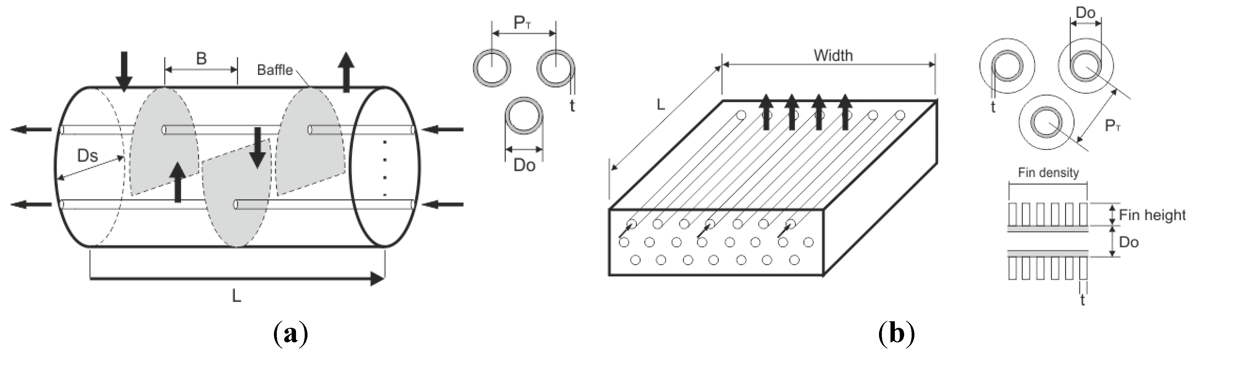
• Evaporator: Evaporation was realized using two parallel evaporators, with one shell/one tube pass configuration. During very low load (<50%) operation, one of the evaporators was fully closed. Both evaporators were sized by determining the shell diameter, and the number of tubes was calculated using “tube counts” based on standardized design parameters described in Table 1. The baffle-spacing was constrained below the shell diameter and maximum-spacing in order to avoid instability caused by vibration. After calculating overall heat transfer coefficients and the total heat transfer area, tube length was computed. By setting the allowable pressure drop on the shell side, the optimum design (or equivalently, shell diameter) with smallest area was selected. This design procedure was also applied to the recuperator.
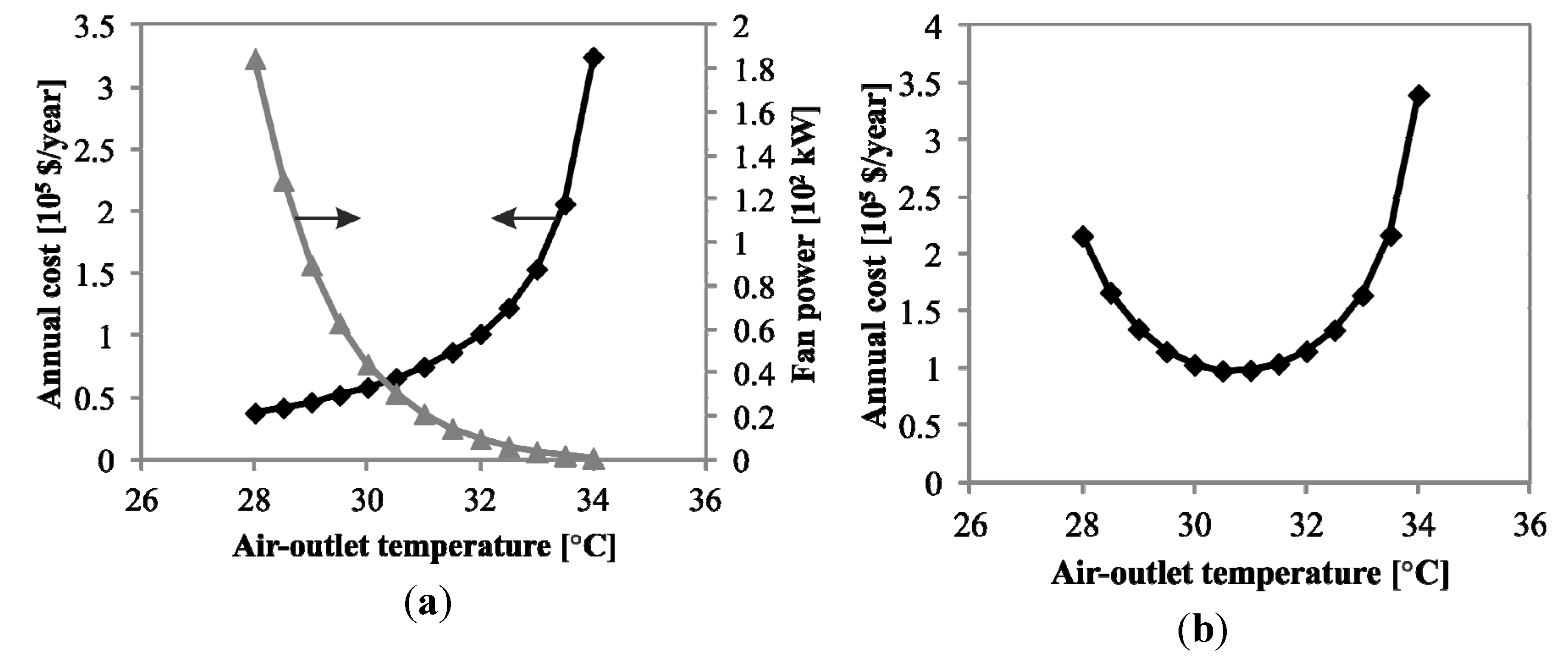
• Condenser: An important preliminary step in the condenser design process is outlet air temperature. This parameter has a major effect on exchanger economics [12]. Increasing the outlet air temperature reduces the amount of air required, which reduces the fan power and, therefore, operating cost. However, it also reduces the air-side heat-transfer coefficient and the mean temperature difference in the exchanger, which increases the size of the unit and, therefore, the capital cost. Consequently, optimization with respect to outlet air temperature (or equivalently, air flow rate) was considered an important aspect of air-cooled condenser design.

The optimum condenser air-outlet temperature (or equivalently, pinch-point) was calculated by minimizing the annual cost function. First derivative of this function with respect to air-outlet temperature determines the minimum annual cost. It can be written as follows:

$$\frac{\partial }{\partial T_{\text{a0,out}}}\left[\text{CRF}\cdot \left(C_{\text{cd}}+C_{\text{F}}\right)+\left(0.01\cdot C_{\text{cd}}+0.03\cdot C_{\text{F}}\right)+CF\cdot P_{\text{F}}\cdot C_{\text{el}}\right]=0$$

(19)

Air-cooled heat exchanger investment cost C_cd and fan investment cost C_F are described in Table 3. The annualization factor, CRF (Capital Recovery Factor) is defined as:

$$CRF=\frac{i{\left(1+i\right)}^y}{{\left(1+i\right)}^y-1}$$

(20)

Heat transfer coefficient and pressure drop were computed from the ratio of design mass flow rate to the reference, which was mass flow rate at air velocity of 3.5 m·s⁻¹, as recommended in the literature [12]. The maintenance cost was assumed to be 1% of the fin/tube heat exchangers cost and 3% of fan-motor cost [22]. CF (capacity Factor) of 0.7, y of 30 years, i of 12%, and electricity price C_el of 0.15 $·kWh⁻¹ were assumed.

Increasing the outlet air temperature increases heat transfer area required and conversely, reduces fan power consumption, as shown in Figure 6a. This trade-off resulted in an optimum annual cost of 130-20 (T_g0-T_a0) at air-outlet temperature of 30.4 °C, approximately 10 K above the inlet air temperature (Figure 6b). Once the optimum air-outlet temperature was established, the heat transfer area (or equivalently, number of cells) and fan capacity were determined.

Table 3. Component cost as function of size.

Component	Cost correlation	Reference
Evaporator	$13,668+658\cdot A^{0.85}$ (Carbon-shell/Stainless-tube)	[22]
Recuperator	$11,256+579\cdot A^{0.8}$ (Carbon-shell/Carbon-tube)	[22]
Air-cooled condensers	$5.6\cdot A$	[23]
Fans	$\left(1887.5+159.95\cdot D_{\text{F}}^2+3.53\cdot D_{\text{F}}+281.25\cdot P_{\text{F}}\right)\cdot N_{\text{F}}$	[23]
Feed-pump	$4900\cdot {\left(P_{\text{P}}/30\right)}^{0.7}$	[24]
Turbine + generator	$\left(91,200\cdot D_{pitch}^{2.1}+50,800\cdot D_{pitch}^3+62,700\cdot D_{pitch}^2\right)+680,900\cdot {\left(P_T/{10}^4\right)}^{0.7}$	[25]
Labor	$0.3\times \text{Total component cost}$	-

Table 3. Component cost as function of size.

Component	Cost correlation	Reference
Evaporator	$13,668+658\cdot A^{0.85}$ (Carbon-shell/Stainless-tube)	[22]
Recuperator	$11,256+579\cdot A^{0.8}$ (Carbon-shell/Carbon-tube)	[22]
Air-cooled condensers	$5.6\cdot A$	[23]
Fans	$\left(1887.5+159.95\cdot D_{\text{F}}^2+3.53\cdot D_{\text{F}}+281.25\cdot P_{\text{F}}\right)\cdot N_{\text{F}}$	[23]
Feed-pump	$4900\cdot {\left(P_{\text{P}}/30\right)}^{0.7}$	[24]
Turbine + generator	$\left(91,200\cdot D_{pitch}^{2.1}+50,800\cdot D_{pitch}^3+62,700\cdot D_{pitch}^2\right)+680,900\cdot {\left(P_T/{10}^4\right)}^{0.7}$	[25]
Labor	$0.3\times \text{Total component cost}$	-

Figure 6. Size optimization based on annual cost of condensers at 130-20 (T_g0-T_a0) design-point.

Figure 6. Size optimization based on annual cost of condensers at 130-20 (T_g0-T_a0) design-point.

4.2. Off-Design Mapping

The off-design performance of the plant may be assessed using the Second Law of thermodynamics by comparing the actual net-power output to the maximum theoretical power that could be produced (energy) from the given geothermal fluid. This involves determining the energy-rate carried into the plant with the incoming geofluid [10]. In order to proportionally evaluate the off-design performance of each design-point, the geofluid mass flow rate at off-design conditions is computed using constant energy rate of 2000 kW at ISO standard ambient temperature of 15 °C:

$${\dot{m}}_{\text{g,in-off}}=\frac{2000\left[\text{kW}\right]}{\left(h_{\text{g,in}}-h_{15°C}\right)-288.15\left[\text{K}\right]\text{}\left(s_{\text{g,in}}-s_{15°C}\right)}\left(\text{off-design}\right)$$

(21)

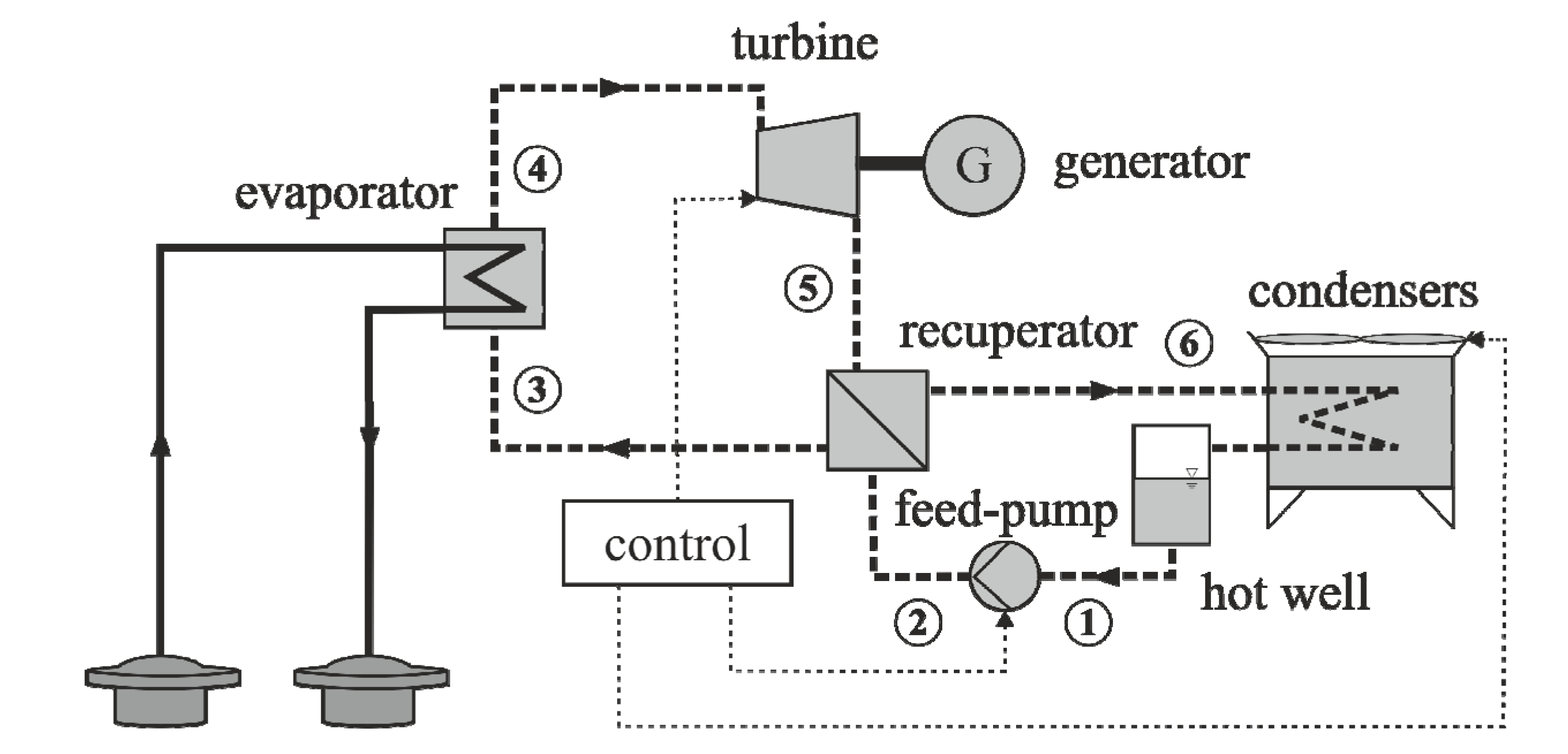
In order to obtain optimal operating point under off-design conditions, a three-variable control strategy was used. First, evaporation pressure was controlled by the turbine nozzle-opening μ_T. Second, superheating/turbine inlet temperature was controlled by pump-speed n_p (isobutane mass flow rate), and third, condensation temperature by the fan-speed n_F (air volumetric flow rate). Constant sub-cooling was imposed by making use of the static pressure head between the pump and the liquid hot-well (Figure 1). Using this control strategy for a modular ORC system, the net power output was maximized while keeping the injection temperature above scaling temperature to avoid scaling, which is described as:

$$\underset{T\text{g,out}\ge 70°C}{\max }\left({\dot{W}}_{\text{T}}-{\dot{W}}_{\text{P}}-{\dot{W}}_{\text{F}}\right)$$

(22)

Scaling temperature is a site-specific problem. It depends on the chemical composition of the geothermal fluid most commonly silica and calcite, and temperature and pressure of the fluid. If the injection temperature of the geofluid falls below this temperature, there is the risk that scales might form in the heat exchanger or the piping system. A minimum bound of 70 °C was selected for this study, based on several works for mid-enthalpy geothermal resources [2,3,26].

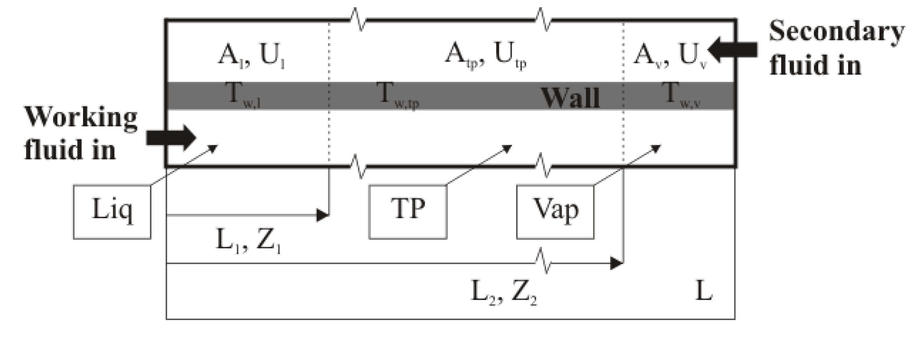
The off-design simulation procedure was realized using a set of three heat balance equations, which were solved by using the Trust-Dogleg Region solver. The heat balance equations are:

(23)

Where f₁ was determined using the three-zone recuperator model, f₂ the evaporator model, and f₃ the condenser model. Pressure drop in the evaporator was minimized to maintain evaporation temperature drop below 5 K. The equations were solved for given operation parameters to simulate the power-cycle. In order to find the optimum operation parameters for each operating condition, CMA-ES was implemented [27].

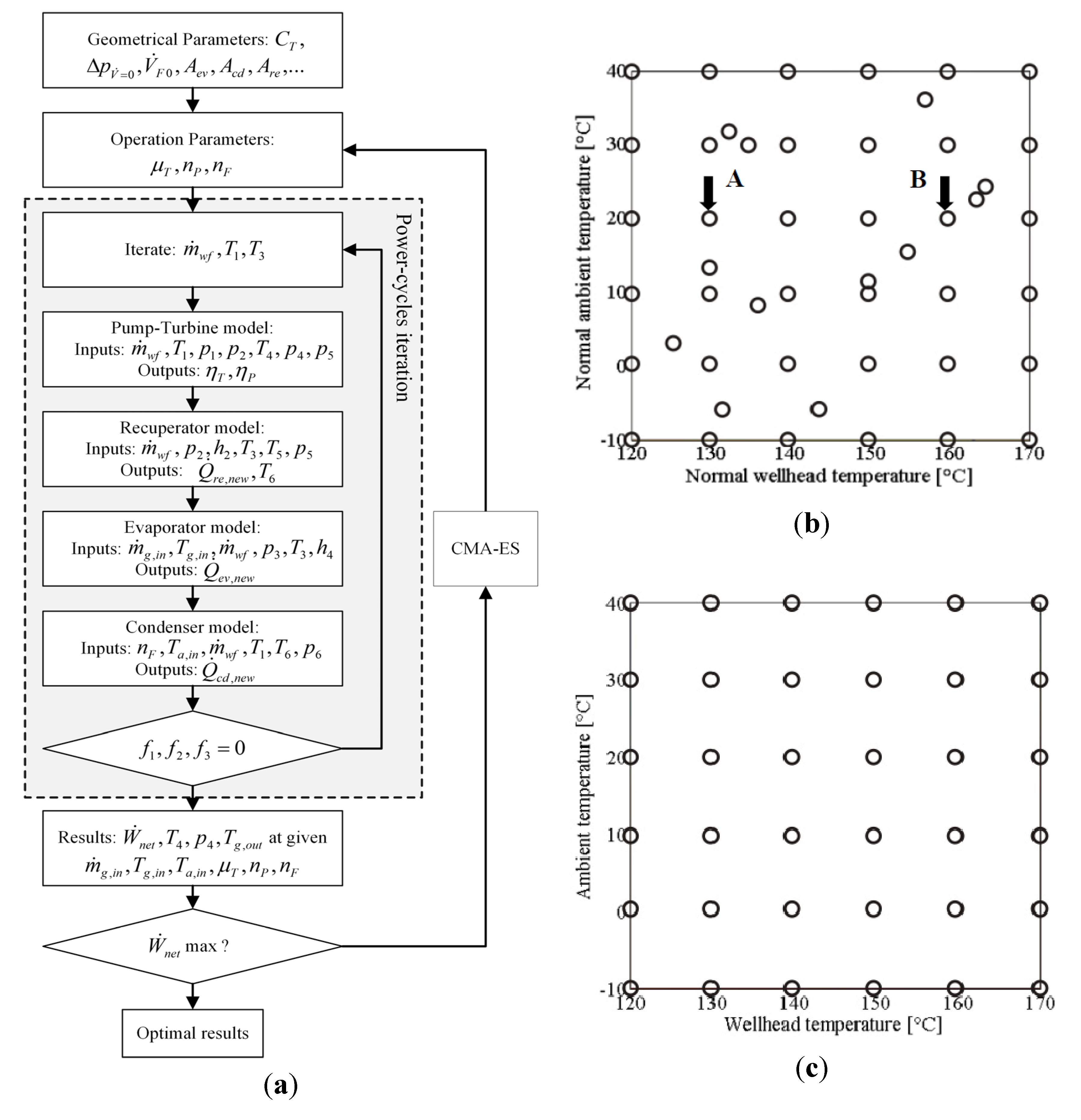
After sizing the components for a design-point, the control variables turbine nozzle, pump and fan rotational speed are optimized to achieve maximum net power output during off-design operating conditions (Figure 7a). The system is assumed to be steady-state for the cycle simulation. The net power output of the plant at 36 off-design wellhead and ambient temperatures (Figure 7c) was evaluated. Gridfit algorithm [28] was then used to interpolate the profiles to produce a 2-D net power output surface contour, as shown in Figure 8.

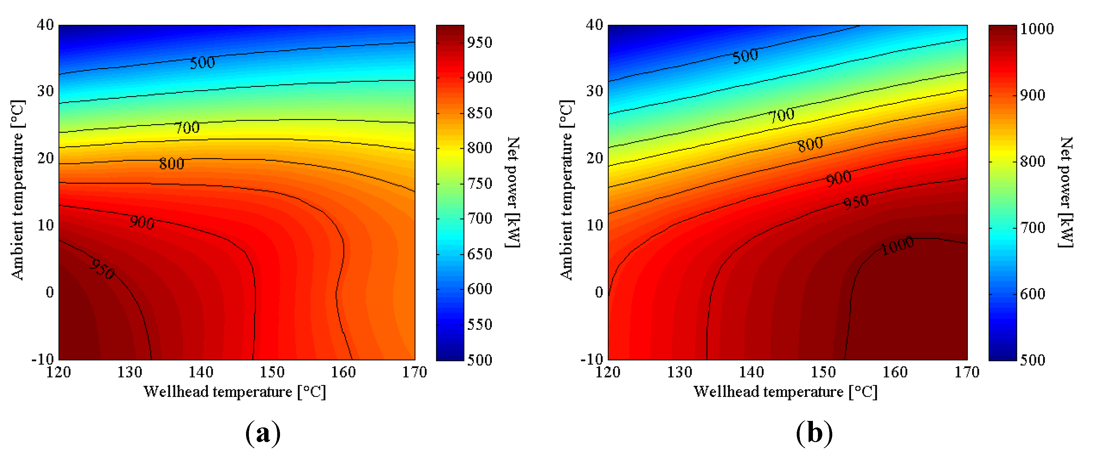
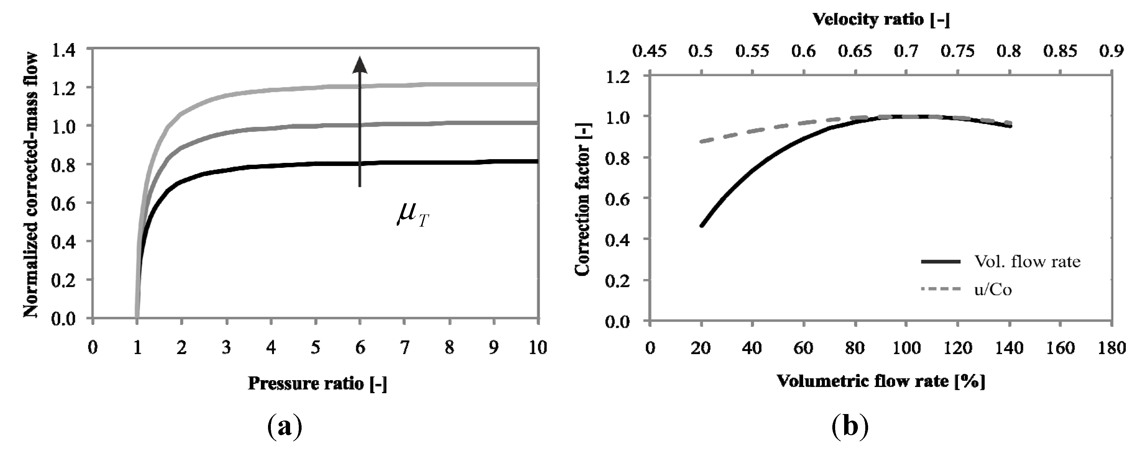
Both design points had constant exergy input, which translated to higher geofluid mass flow rate at lower wellhead temperatures, as previously described in Equation (20). The maximum net power output (978 kW) occurred at T_g,in = 120 °C, T_a,in = −10 °C for 130-20 (Point A, Figure 7b). While maximum net power output (1025 kW) occurred at T_g,in = 160 °C, T_a,in = −10 °C for 160-20 (Point B, Figure 7b). It can be observed contradictory net power-output trend between the two design points. For 130-20, by increase of geofluid temperature, the net power output decreases, especially at lower ambient temperature. In contrary, for 160-20, the net power output showed an opposite trend. This was affected mainly on the turbine isentropic efficiency characteristic at off-design. The nominal (design) isentropic enthalpy drop was lower and the nominal volumetric flow rate was higher for 130-20. Hence, if the plant was operated at higher wellhead temperature which has higher enthalpy drop and lower flow rate, the turbine isentropic efficiency would steeply deteriorated (see Figure 5b).

It is also important to note the different net-power dependencies on ambient temperature. When investigating at a constant T_g,in at the optimum point, the net power output decreased by 65.1% for 130-20 and 44.5% for 160-20 between −10 °C and 40 °C.

Figure 7. (a) Off-design optimization procedure for a design-point (T_g0-T_a0) and operating condition (${\dot{m}}_{\text{g}}$,T_g,in, T_a,in); (b) Design-point grid; and (c) Off-design grid.

Figure 7. (a) Off-design optimization procedure for a design-point (T_g0-T_a0) and operating condition (${\dot{m}}_{\text{g}}$,T_g,in, T_a,in); (b) Design-point grid; and (c) Off-design grid.

Figure 8. Off-design maps of net power output for (a) 130-20; (b) 160-20.

Figure 8. Off-design maps of net power output for (a) 130-20; (b) 160-20.

4.3. Annual Simulation and Thermo-Economic Selection

The system is assumed to be at steady-state for the annual simulations, and the heat loss in each component is neglected. The cycle performance is calculated in each time step of 1 h. The steady-state approximation is considered to be reasonably accurate since ambient temperature change is slower than the heat exchanger dynamics in the system. Thermal-economic optimization then was conducted to measure the trade-off between annual energy utilization and cost. Specific component costs are described in Table 3; however, the cost correlations listed are not the exact economic values, since cost can vary strongly depending on market. Nonetheless, the values presented here used as a means to convert geometric design parameters into economic value, and correlations are taken from actual literatures [22,23,24].

The turbine cost was taken from a model developed by Barber-Nichols [25]. The correlations are corrected to current cost by using the Chemical Engineering Plant Cost Index (CEPCI) [29]. The parameters, A, D_F, N_F, P_F, P_T, and P_P in Table 3 were determined directly from the sizing results. The turbine pitch (average wheel) diameter, D_pitch, was derived from a universal functional relationship, for optimum stage efficiency [30] as:

$${\dot{V}}_{5,design}=0.177\cdot D_{pitch}\cdot \sqrt{\Delta h_{is0}}$$

(24)

Two economic criteria were computed: specific investment cost (SIC) and mean cash flow (MCF). SIC is a typical parameter used in thermal-economic optimization, and is defined as:

$$\text{SIC}\left[\$\cdot {\text{kW}}^{-1}\right]=\frac{\text{Component cost+Labor cost}}{\text{Averaged annual capacity}\left({\overline{P}}_{\text{net}}\right)}$$

(25)

where ${\overline{P}}_{\text{net}}$ is mean annual net power output calculated as the averaged sum of annual energy production for each wellhead temperature (in kWh) divided by 7008 h. MCF measures the productivity of the power-plant, and is computed as:

$$\text{MCF}\left[\$\cdot {\text{year}}^{-1}\right]=\text{Revenue}-\text{CRF}\cdot \left(\text{Component cost}+\text{Labor cost}\right)-C_{\text{O\&M}}-\text{Well cost}$$

(26)

where Revenue = ${\overline{P}}_{\text{net}}$ × C_el and the three later terms are particularly annualized cost of electricity, i.e., investment cost, annual operation and maintenance costs of the overall plant which are assumed to be 4% of the investment cost [31], and well cost. Well cost accounted for the geofluid-pumping and drilling costs, which are arbitrary values dependent on site-specific characteristics. It was assumed a well cost equal to zero since it will only shift the MCF to a lower value, and result in an unchanged optimum design-point. The three climates temperate, tropical and dry—chosen for annual simulation were sampled from existing geothermal sites: Upper-Rhine Graben, Germany (temperate climate), Kamojang, Indonesia (tropical climate), and Birdsville, Australia (dry climate). The temperature distributions of each climate are shown in Table 4.

Table 4. Ambient temperature distribution of three climates during generic year.

Temperature [°C]	Temperate climate ( Tav = 11.6 °C)		Tropical climate ( Tav = 19.9 °C)		Dry climate ( Tav = 25.1 °C)
	Number of hours	% hours	Number of hours	% hours	Number of hours	% hours
−10	266	3.0	0	0	0	0
0	2438	27.8	0	0	17	0.2
10	2926	33.4	351	4.0	1195	13.6
20	2159	24.6	7934	90.6	3139	35.8
30	726	8.3	475	5.4	3154	36.0
40	245	2.8	0	0	1254	14.3

Table 4. Ambient temperature distribution of three climates during generic year.

Temperature [°C]	Temperate climate ( Tav = 11.6 °C)		Tropical climate ( Tav = 19.9 °C)		Dry climate ( Tav = 25.1 °C)
	Number of hours	% hours	Number of hours	% hours	Number of hours	% hours
−10	266	3.0	0	0	0	0
0	2438	27.8	0	0	17	0.2
10	2926	33.4	351	4.0	1195	13.6
20	2159	24.6	7934	90.6	3139	35.8
30	726	8.3	475	5.4	3154	36.0
40	245	2.8	0	0	1254	14.3

The annual energy production was calculated using the hourly variation of T_a.in at each site. This calculation only includes cost, which varies significantly according to the component size. The remaining costs, such as piping, instrumentation and working fluid, were excluded.

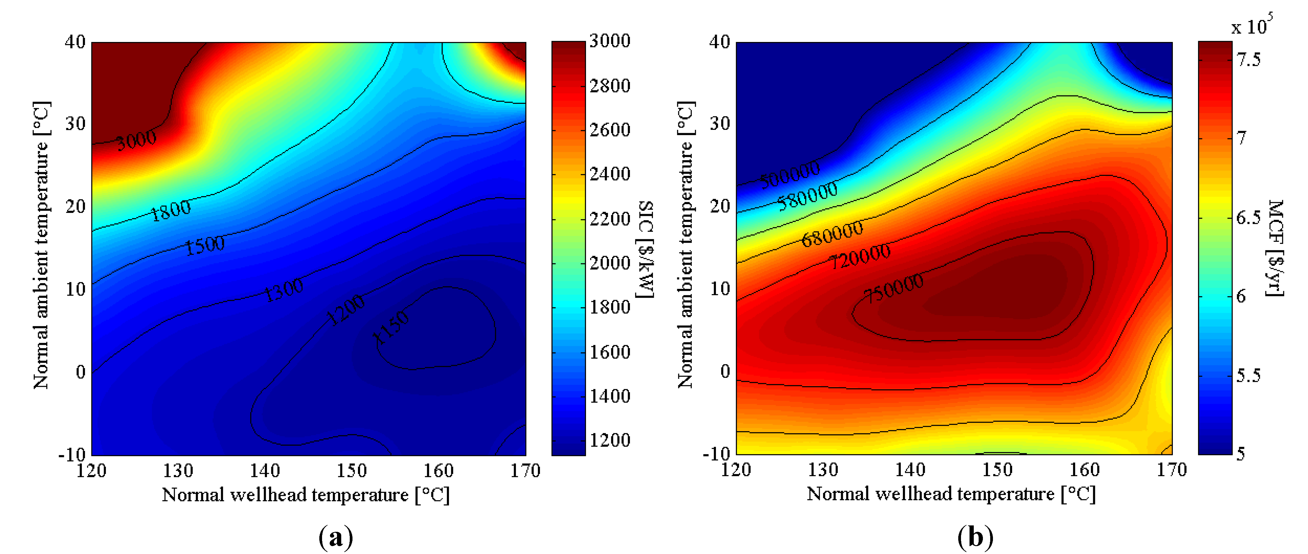
Under the conditions assumed for the temperate climate, the optimum points of SIC and MCF optimization was different (Figure 9). SIC minimization yielded 160-6, with a cost value of 1133 $·kW⁻¹, while MCF maximization yielded 153-10, with a cost value of 761,350 $·year⁻¹. The SIC and MCF showed large variation, ranging from 1133 $·kW⁻¹ to 5296 $·kW⁻¹, and 92,224 $·kW⁻¹ to 761,350 $·kW⁻¹, respectively.

Figure 9. Design-point based on minimizing SIC (a) and maximizing MCF (b) in temperate climate.

Figure 9. Design-point based on minimizing SIC (a) and maximizing MCF (b) in temperate climate.

Comparing the two objective functions, SIC minimization resulted in values 5.1%–7.1% lower, relative to plants based on maximizing MCF. By maximizing MCF, values were 2.1%–10.8% higher compared to when SIC was minimized. The temperate climate had the lowest SIC minimum and highest MCF maximum, followed by the tropical and then the dry climate. The optimization results are reported in Table 5. Using SIC minimization, the optimum normal wellhead temperature was constant at T_g0 of 160 °C across the three climates, and optimum T_a0 followed lower temperatures of 6 °C, 10 °C and 10 °C. While in MCF maximization, optimum T_g0 was 153 °C, 163 °C and 163 °C, and T_a0 followed average temperatures of 10 °C, 22 °C and 23 °C, respectively. 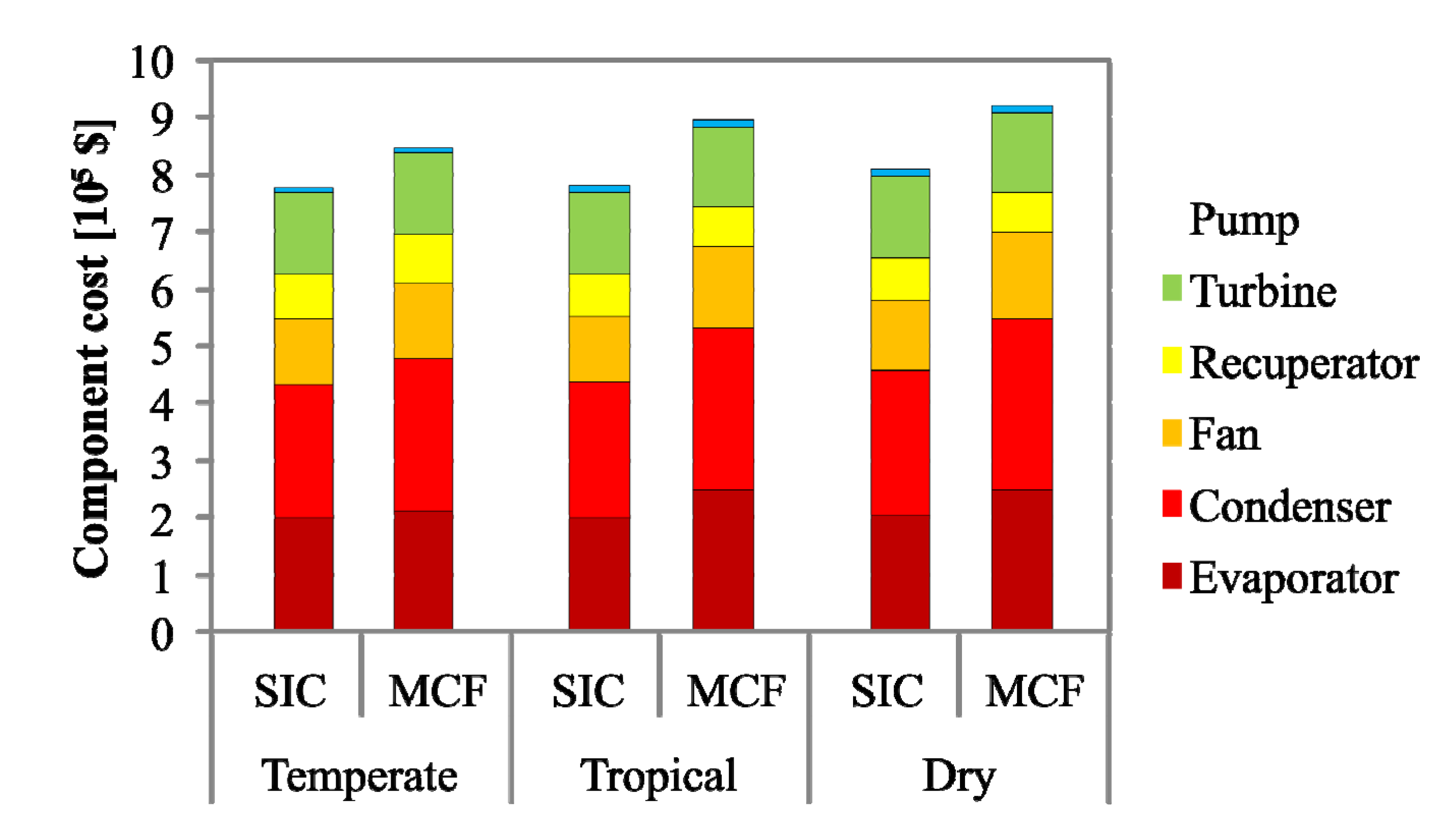Figure 10 shows relative component costs among the three climates.

Table 5. SIC and MCF for each optimal design-point and climate type.

Sizing	Design-point [°C]		SIC [$·kW−1]	MCF [$·year−1]
	Tg0	Ta0
Temperate climate
SIC minimization	160	6	1,133	745,770
MCF maximization	153	10	1,198	761,350
Tropical climate
SIC minimization	160	10	1,303	642,070
MCF maximization	163	22	1,403	683,120
Dry climate
SIC minimization	161	10	1,520	524,230
MCF maximization	163	23	1,601	580,800

Table 5. SIC and MCF for each optimal design-point and climate type.

Sizing	Design-point [°C]		SIC [$·kW−1]	MCF [$·year−1]
	Tg0	Ta0
Temperate climate
SIC minimization	160	6	1,133	745,770
MCF maximization	153	10	1,198	761,350
Tropical climate
SIC minimization	160	10	1,303	642,070
MCF maximization	163	22	1,403	683,120
Dry climate
SIC minimization	161	10	1,520	524,230
MCF maximization	163	23	1,601	580,800

Figure 10. Relative component cost comparison between SIC and MCF optimization under three different climate types.

Figure 10. Relative component cost comparison between SIC and MCF optimization under three different climate types.

SIC minimization resulted in a investment cost that was 8.2%–13% lower than plants designed using maximized MCF. The cooling-system cost (condenser heat exchangers, fans) dominated the total investment cost. For plants with minimized SIC, the cooling-system cost was 12.5%–16.7% lower than those designed using maximized MCF. In contrast, MCF maximization resulted in a higher mean annual net-power 3.4%–12.7%. This improvement was based on the optimal number of cells and fan capacity, which maintain low condensation pressure and, in turn, result in higher power.

5. Conclusions

The main conclusions of this work are as follows:

• Using the modularization technique described in this paper, design optimization under three different climates (temperate, tropical, and dry) was derived. Using SIC minimization, the normal ambient temperatures were driven by the lower temperature. Using MCF maximization, the normal ambient temperatures were driven by average temperature in each climate region.
• When SIC minimization and MCF maximization were compared, average net-power based on MCF maximization was higher. Although investment cost was slightly higher, the revenue or equivalently, the energy utilization was considerably improved. Consequently, MCF maximization is proposed as an optimization function.
• Concerning the various components analyzed here, the condenser and fan size had the greatest influence on average net power output. The main feature in MCF maximization design was increased size of the cooling-system, which helped maintain low condensation pressure. Using isobutane, the condenser cost amounted to 35%–38% of the investment cost. Enhancing the heat transfer of cooling system technology will reduce the condenser size and, most importantly, the ORC investment cost.

References

1. Stefansson, V. World Geothermal assessment. In Proceedings of World Geothermal Congress 2005, Antalya, Turkey, 24–29 April 2005.
2. Aneke, M.; Agnew, B.; Underwood, C. Performance analysis of the Chena binary geothermal power plant. Appl. Therm. Eng. 2011, 31, 1825–1832. [Google Scholar] [CrossRef]
3. Bäumer, R.; Kalinowski, I.; Röhler, E.; Schöning, J.; Wachholz, W. Construction and operating experience with the 300-MW THTR nuclear power plant. Nucl. Eng. Des. 1990, 121, 155–166. [Google Scholar] [CrossRef]
4. Dahmus, J.B. Modular Product Architecture. Des. Stud. 2001, 22, 409–424. [Google Scholar] [CrossRef]
5. Quoilin, S.; Broek, M.V.D.; Declaye, S.; Dewallef, P.; Lemort, V. Techno-economic survey of Organic Rankine Cycle (ORC) systems. Renew. Sustain. Energy Rev. 2013, 22, 168–186. [Google Scholar]
6. Valdimarsson, P. New Development in the ORC Technology. In Proceedings of Short Course VI on Utilization of Low- and Medium-Enthalpy Geothermal Resources and Financial Aspects of Utilization, Santa Tecla, El Salvador, 23–29 March 2014.
7. Manente, G.; Toffolo, A.; Lazzaretto, A.; Paci, M. An Organic Rankine Cycle off-design model for the search of the optimal control strategy. Energy 2013, 58, 97–106. [Google Scholar] [CrossRef]
8. Gabbrielli, R. A novel design approach for small scale low enthalpy binary geothermal power plants. Energy Convers. Manag. 2012, 64, 263–272. [Google Scholar] [CrossRef]
9. Augustine, C. Hydrothermal Spallation Drilling and Advanced Energy Conversion Technologies for Engineered Geothermal Systems. Ph.D. Thesis, Massachusetts Institute of Technology, Cambridge, MA, USA, 2009. [Google Scholar]
10. DiPippo, R. Geothermal Power Plants: Principles, Applications, Case Studies, and Environmental Impact; Butterworth-Heinemann: Waltham, MA, USA, 2008. [Google Scholar]
11. Hernandez-Galan, J.L.; Alberto Plauchu, L. Determination of·fouling factors for shell-and-tube type heat exchangers exposed to los azufres geothermal fluids. Geothermics 1989, 18, 121–128. [Google Scholar] [CrossRef]
12. Serth, R.W. Process Heat Transfer: Principles and Applications; Elsevier: Amsterdam, The Netherlands, 2007. [Google Scholar]
13. Doo, G.H. Modeling and Experimental Study of Evaporating Two-Phase Flow on the Shellside of Shell-and-Tube Heat Exchanger. Ph.D. Thesis, University of Strathcylde, Scotland, UK, 2005. [Google Scholar]
14. Dobson, M.K.; Chato, J.C. Condensation in Smooth Horizontal Tubes. J. Heat Trans. 1998, 120, 193–213. [Google Scholar]
15. Engineering Data Book; Gas Processor Suppliers Association (GPSA): Tulsa, OK, USA, 2004.
16. Shekun, G.D. Approximating the efficiency characteristics of blade pumps. Therm. Eng. 2007, 54, 886–891. [Google Scholar] [CrossRef]
17. Dixon, S.L. Fluid Mechanins and Thermodynamics Turbomachinery; Butterworth Heinemann: Waltham, MA, USA, 2002. [Google Scholar]
18. Ghasemi, H.; Paci, M.; Tizzanini, A.; Mitsos, A. Modeling and optimization of a binary geothermal power plant. Energy 2013, 50, 412–428. [Google Scholar]
19. Frick, S.; Saadat, A.; Kranz, S. Cooling of Low-Temperature Power Plants—Challenges for the Example of Geothermal Binary Power Plants. In Proceedings of 6th International Symposium on Cooling Towers, Cologne, Germany, 20–23 June 2012.
20. Air-Cooled Condenser Design, Specification, and Operation Guidelines; The Electric Power Research Institute: Palo Alto, CA, USA, 2005.
21. He, C.; Liu, C.; Gao, H.; Xie, H.; Li, Y.; Wu, S.; Xu, J. The optimal evaporation temperature and working fluids for subcritical Organic Rankine Cycle. Energy 2012, 38, 136–143. [Google Scholar]
22. Taal, M.; Bulatov, I.; Klemeš, J.; Stehlik, P. Cost estimation and energy price forecasts for economic evaluation of retrofit projects. Appl. Therm. Eng. 2003, 23, 1819–1835. [Google Scholar] [CrossRef]
23. Alinia Kashani, A.H.; Maddahi, A.; Hajabdollahi, H. Thermal-economic optimization of an air-cooled heat exchanger unit. Appl. Therm. Eng. 2013, 54, 43–55. [Google Scholar] [CrossRef]
24. Quoilin, S.; Declaye, S.; Tchanche, B.F.; Lemort, V. Thermo-economic optimization of waste heat recovery Organic Rankine Cycles. Appl. Therm. Eng. 2011, 31, 2885–2893. [Google Scholar] [CrossRef]
25. Milora, S.L.; Tester, J.W. Geothermal Energy as a Source of Electric Power; The MIT Press: Cambridge, MA, USA, 1976. [Google Scholar]
26. Astolfi, M.; Romano, M.C.; Bombarda, P.; Macchi, E. Binary ORC (Organic Rankine Cycles) power plants for the exploitation of medium–low temperature geothermal sourcesPart B: Techno-economic optimization. Energy 2014, 66, 435–446. [Google Scholar]
27. Hansen, N. Towards a New Evolutionary Computation. In Studies in Fuzziness and Soft Computing; Springer: Berlin, Germany, 2006; pp. 75–102. [Google Scholar]
28. Keim, D.A.; Herrmann, A. The Gridfit Algorithm: An Efficient and Effective Approach to Visualizing Large Amounts of Spatial Data. In. In Proceedings of Visualization’s 98 Research, Triangle Park, NC, USA, 18–23 October 1998; pp. 181–188.
29. Spang, B.; Roetzel, W. C6 Costs and Economy of Heat Exchangers. In VDI Heat Atlas; Springer: Berlin, Germany, 2010. [Google Scholar]
30. Balje, O.E. A Study on Design Criteria and Matching of Turbomachines. J. Eng. Gas Turbines Power 1962, 84, 83–102. [Google Scholar]
31. Entingh, D.J.; Eyob, E.; McLarty, L. Small Geothermal Electric Systems for Remote Powering; Geothermal Resource Council: Davis, CA, USA, 1994. [Google Scholar]